Conserved vectors and symmetry solutions of the Landau–Ginzburg–Higgs equation of theoretical physics
Chaudry Masood Khalique
, ∗
,
Mduduzi Yolane Thabo Lephoko
Expand
Material Science, Innovation and Modelling Research Focus Area, Department of Mathematical Sciences, North-West University, Mafikeng Campus, Private Bag X 2046, Mmabatho 2735, South Africa
∗Author to whom any correspondence should be addressed.
This paper is devoted to the investigation of the Landau–Ginzburg–Higgs equation (LGHe), which serves as a mathematical model to understand phenomena such as superconductivity and cyclotron waves. The LGHe finds applications in various scientific fields, including fluid dynamics, plasma physics, biological systems, and electricity-electronics. The study adopts Lie symmetry analysis as the primary framework for exploration. This analysis involves the identification of Lie point symmetries that are admitted by the differential equation. By leveraging these Lie point symmetries, symmetry reductions are performed, leading to the discovery of group invariant solutions. To obtain explicit solutions, several mathematical methods are applied, including Kudryashov’s method, the extended Jacobi elliptic function expansion method, the power series method, and the simplest equation method. These methods yield solutions characterized by exponential, hyperbolic, and elliptic functions. The obtained solutions are visually represented through 3D, 2D, and density plots, which effectively illustrate the nature of the solutions. These plots depict various patterns, such as kink-shaped, singular kink-shaped, bell-shaped, and periodic solutions. Finally, the paper employs the multiplier method and the conservation theorem introduced by Ibragimov to derive conserved vectors. These conserved vectors play a crucial role in the study of physical quantities, such as the conservation of energy and momentum, and contribute to the understanding of the underlying physics of the system.
Chaudry Masood Khalique, Mduduzi Yolane Thabo Lephoko. Conserved vectors and symmetry solutions of the Landau–Ginzburg–Higgs equation of theoretical physics[J]. Communications in Theoretical Physics, 2024, 76(4): 045006. DOI: 10.1088/1572-9494/ad2a63
1. Introduction
Nonlinear partial differential equations (NLPDEs) are extensively employed in the fields of science and engineering to represent and study a wide range of nonlinear phenomena encountered in practical applications [1–13]. These equations play a crucial role in modeling various scenarios, including fluid dynamics problems, wave propagation in complex media, seismic wave analysis, and the characterization of optical fibers. The versatility and applicability of NLPDEs enable researchers and engineers to gain valuable insights into complex physical phenomena and devise effective strategies to address real-world challenges. Numerous mathematical and physical NLPDEs have been investigated in the literature and, currently, mathematicians are tackling even more. For instance, in their research, Zhang and Xiao [8] utilized an undetermined coefficient method to study the (2+1)-dimensional generalized Hirota–Satsuma–Ito equation, which describes the propagation of unidirectional shallow-water waves. They focused on obtaining double-periodic soliton solutions. In a separate study, Rao et al [9] utilized the Cole–Hopf algorithm to analyze the (2+1)-dimensional modified dispersive water-wave system, and obtained its exact solutions. Zhang and Wang [10] employed various methods, including the simplified extended tanh-function method, variational method, and He’s frequency formulation method, to investigate the Fokas system that arises in monomode optical fibers. Through their research, they obtained fifteen sets of soliton solutions. Wang and Liu [11] investigated the new coupled Konno–Oono equation that plays a key role in the magnetic field by applying the Exp-function method to find its analytical solutions.
The pursuit of accurate solutions for NLPDEs holds considerable importance within the realm of applied mathematics. These precise solutions assume a pivotal role in comprehending the qualitative and quantitative attributes of nonlinear phenomena. Despite the existence of diverse classes of intriguing exact solutions, such as soliton and traveling wave solutions, their construction usually requires specialized mathematical techniques due to the nonlinearity inherent in their dynamic nature. However, the presence of nonlinearity in NLPDEs presents a formidable challenge to discovering explicit, specific, or general solutions. Consequently, various robust techniques have been proposed and developed to derive analytical solutions for nonlinear problems.
Stating a few of the well-established techniques, we have the ansatz technique [14], the extended homoclinic-test approach [15], the generalized unified technique [16], the tanh-coth method [17], the exp (−Φ(η))-expansion technique [18], the Bäcklund transformation approach [19], the Cole–Hopf transformation approach [20], the Painlevé expansion approach [21], the mapping and the extended mapping approaches [22], the homotopy perturbation approach [23], the rational expansion method [24], the simplest and the extended simplest equation techniques [25], the F-expansion approach [26], Hirota’s technique [27], Lie symmetry analysis [28, 29], the Darboux transformation technique [30], the exponential function technique [31], Kudryashov’s technique [32], the tanh-function method [33], and the bifurcation approach [34].
Conservation laws are of significant importance in the analysis of differential equations. One practical application of this is the assessment of the integrability of a partial differential equation via examination of its conservation laws [29]. Furthermore, conservation laws serve as a tool for assessing the precision of numerical solution techniques, help identify special solutions that have important physical properties, and can be used to reduce the number of unknowns in a problem, making it easier to solve [29]. Thus, this is the reason mathematicians find it useful to determine the conservation laws for a given differential equation (DE) [35, 36]. A novel category of nonlinear evolution equations (NLEEs), featuring a nonlinear term of arbitrary order represented in the form
were introduced by Chen et al [37], where a1, a2, a3, a4, and p ≠ 1 are arbitrary constants. When p takes a different constant, a different equation will be constructed. These include the sine-Gordon equation, Duffing equation, and the Klein–Gordon equation. Infact, when p = 3, a4 = 0 we get the NLEE
with u = u(t, x) representing the electrostatic potential of the ion-cyclotron wave, and a and b are constants [38, 39]. The LGHe (1.3) is used to understand the concepts of superconductivity and cyclotron waves, which have applications in a variety of fields, including medicine, plasma physics, chemistry, biology, electricity-electronics, and transportation [40].
In [39], the modified exponential function approach was used to obtain the solution of the LGHe (1.3) that were of the hyperbolic, trigonometric, and rational functions forms. Barman et al [41] employed the extended tanh method and applied the solitary wave hypothesis to obtain explicit traveling wave solutions. They achieved this by assigning various specific values to the parameters involved in the equations. Bekir and Ünsal [38] obtained solitary and periodic wave, and exponential solutions via the first integral method with the computerized symbolic computation system Maple. Islam and Akbar [42] utilized the improved Bernoulli sub-equation function method to successfully establish stable general, broad-ranging, typical, and fresh soliton solutions to the LGHe. Iftikhar et al [43] used the $(G^{\prime} /G,1/G)$-expansion method to gain traveling wave solutions. Recently, Ahmad et al [44] obtained exact solutions of the LGHe in terms of elliptic Jacobi functions by applying the power index method using function conversion. Asjad et al [45] obtained solitary wave solitons by utilizing the generalized projective Riccati method.
Motivated by the existing literature, this research endeavors to address the LGHe (1.3) using five distinct and efficient techniques: the Lie symmetry technique, Kudryashov’s technique, the extended Jacobi elliptic function technique, the power series method, and the simplest equation approach. The primary objective of this study is to generate a new multitude of exact solutions for the LGHe (1.3). Additionally, the dynamical behaviour of solitary wave profiles for select soliton solutions will be demonstrated through numerical simulations by employing three-dimensional and density plots. Notably, we assert that the evolutionary dynamics and physical interpretation of the acquired exact soliton solutions are highly intriguing and offer valuable insights for further physical propositions. Importantly, the majority of the derived exact soliton solutions are new and, to the best of our knowledge, have not been previously reported in the literature. Finally, for the first time, we establish the conservation laws associated with the underlying model by employing the multiplier method and Ibragimov’s theorem.
2. Lie symmetry analysis of the LGHe
In this section we first use the algorithm for the computation of Lie point symmetries of the LGHe (1.3) and generate its Lie point symmetries. Thereafter, we utilize them to construct exact solutions for equation (1.3).
2.1. Lie point symmetries of the LGHe
Let us consider the one-parameter Lie group of infinitesimal transformations, namely,
where α denotes the parameter of the group, while τ, ξ, and η represent the infinitesimals of the transformations. Utilizing a one-parameter Lie group of infinitesimal transformations that satisfy certain invariant conditions [29], the solution space (t, x, u) of the LGHe (1.3) remains invariant and can be transformed into another space $(\tilde{t},\tilde{x},\tilde{u})$. Imploring the vector field
the symmetry group of the LGHe (1.3) will be found. We recall that equation (2.4) is a symmetry of the LGHe (1.3), provided that the invariance condition
$\begin{eqnarray}{{pr}}^{(2)}{ \mathcal W }({u}_{{tt}}-{u}_{{xx}}+{a}^{2}u+{b}^{2}{u}^{3}){| }_{(1.3)}=0,\end{eqnarray}$
holds. Here, ${{pr}}^{(2)}{ \mathcal W }$ denotes the second prolongation of ${ \mathcal W }$ [29] defined by
$\begin{eqnarray}{{pr}}^{(2)}{ \mathcal W }={ \mathcal W }+{\zeta }_{t}{\partial }_{{u}_{t}}+{\zeta }_{x}{\partial }_{{u}_{x}}+{\zeta }_{{xx}}{\partial }_{{u}_{{xx}}}+{\zeta }_{{tt}}{\partial }_{{u}_{{tt}}},\end{eqnarray}$
Expanding the determining equation (2.5) and separating it into its constituent derivatives of u, we obtain an overdetermined system of eight homogeneous linear partial differential equations
with c1, c2, and c3 being arbitrary constants. Thus, we have three symmetries
$\begin{eqnarray}{{ \mathcal W }}_{1}=\displaystyle \frac{\partial }{\partial t},\,{{ \mathcal W }}_{2}=\displaystyle \frac{\partial }{\partial x},\,{{ \mathcal W }}_{3}=x\displaystyle \frac{\partial }{\partial t}+t\displaystyle \frac{\partial }{\partial x}.\end{eqnarray}$
The LGHe (1.3) admits a three-dimension Lie algebra L3, which is spanned by the vector fields ${{ \mathcal W }}_{1},{{ \mathcal W }}_{2},{{ \mathcal W }}_{3}$, as defined in equation (2.8).
The group transformations related to the Lie algebra L3 are given as
with α1,…,α3 representing real numbers. Thus, we can state the following theorem.
If $u={ \mathcal N }(t,x)$ is a solution of the LGHe (1.3), then by using the one-parameter symmetry groups ${G}_{i}\,(i=1,2,3)$, we have new solutions given by
$\begin{eqnarray*}\begin{array}{rcl}u & = & {{ \mathcal N }}_{1}(t-{\alpha }_{1},x),\\ u & = & {{ \mathcal N }}_{2}(t,x-{\alpha }_{2}),\\ u & = & {{ \mathcal N }}_{3}(t\cosh ({\alpha }_{3})-x\sinh ({\alpha }_{3}),x\cosh ({\alpha }_{3})-t\sinh ({\alpha }_{3})).\end{array}\end{eqnarray*}$
2.2. Symmetry reduction of the LGHe
This section focuses on the utilization of the infinitesimal symmetries obtained in the previous section to determine the similarity variables and exact solutions of the LGHe (1.3). This involves solving the characteristic equation, which is akin to solving the invariant surface conditions.
Reduction 1. The symmetry ${{ \mathcal W }}_{1}={\partial }_{t}$ yields two invariants u = G(q), q = x. Utilization of these invariants transforms the LGHe (1.3) to the reduced nonlinear ordinary differential equation (NLODE)
Reduction 4. Finally, the linear combination ${{ \mathcal W }}_{1}+c{{ \mathcal W }}_{2}\,={\partial }_{t}+c{\partial }_{x}$, where c is the wave speed, transforms the LGHe (1.3) to the reduced NLODE
We employ various methods to find exact solutions for the reduced NLODEs (2.9), (2.10), (2.11), and (2.12). These methods allow us to explore different approaches to obtaining diverse solutions for the reduced equations.
3.1. Solutions of equation (1.3) using Kudryashov's technique
We present a solution to equation (1.3) using Kudryashov’s method [46]. This method is widely used to obtain closed-form solutions to NLPDEs. The first step involves reducing the NLPDE (1.3) to an NLODE, which we have already accomplished in the previous section. Thus, we will be working with the NLODE (2.9). We assume that the solution to equation (2.9) can be expressed as
which represent the steady state solutions of equation (1.3).
3.2. Solutions of equation (1.3) via application of the extended Jacobi elliptic function technique
In this section, we employ the extended Jacobi elliptic function expansion method, as outlined in [47–49], to solve the NLODE (2.10) and obtain the cnoidal, snoidal, and dnoidal wave solutions of the LGHe (1.3). The methodology involves representing the solution of the NLODE as
denote the cosine-amplitude function, the sine-amplitude function, and delta amplitude function, respectively. The aforementioned serve as solutions to the NLODEs
where A−1, A0, and A1 are constants that need to be determined. By substituting the given expression for G(t) into equation (2.10) and employing equation (3.22), we obtain an equation that can be separated into different powers of G(t) and that yields seven distinct algebraic equations
where it should be noted that as ω → 1, $\mathrm{cn}(t| \omega )\to {\rm{sech}} (t)$. Therefore, the general solution for solution sets 2 and 3 is a hyperbolic function, which can be expressed as
3.2.2. Sine-amplitude periodic wave solutions of equation (1.3)
In a similar manner, we derive snoidal wave solutions for equation (1.3). It is important to note that the balancing procedure results in M = 1. We utilize the NLODE presented in equation (3.23), with its solution given by equation (3.20). Following a similar procedure to that described previously, we obtain the following set of seven distinct algebraic equations:
As before, we now proceed to obtain dnoidal wave solutions for the LGHe (1.3). We employ the NLODE stated in (3.24), whose solution is provided by (3.21), and derive the set of seven algebraic equations
3.3. Solution of equation (1.3) using the power series method
The power series solution technique [50–52] for DEs is now employed to construct solutions of the LGHe (1.3). Power series methods have proven to be effective in addressing challenging DEs, encompassing a wide range, from difficult semi-linear to complex nonlinear differential equations. Hence, in this section, we aim to obtain the exact analytical solutions for the NLODE (2.11) using the power series technique. Consequently, we employ the formal series solution
Utilizing equations (3.30), (3.31), and (3.32), it is possible to determine all the coefficients ρn(n ≥ 2) of the power series, equation (3.26). For arbitrarily selected constants ρ0, ρ1, ρ2, and ρ3, the remaining terms can also be determined in a unique manner through successive application of equations (3.30), (3.31), and (3.32).
Convergence of the power series solution
Now, we shall provide proof of the convergence of the power series solution, equation (3.26). Hence, we introduce a new series
The series, equation (3.33), is a majorant series of equation (3.26).
To establish that the new series, equation (3.33), serves as a majorant series for equation (3.26), it suffices to demonstrate that $\left|{\rho }_{n}\right|\leqslant {q}_{n}$, for $n=0,1,2,\cdots .$ Without loss of generality, from equation (3.32), we establish the following:
It is sufficient to show that ${ \mathcal P }(z,\lambda )$ is analytic in the neighborhood of $\left(0,{q}_{0}\right)$. From equation (3.36), it is evident that
$\begin{eqnarray*}{ \mathcal P }\left(0,{q}_{0}\right)=0,\quad {{ \mathcal P }}_{\lambda }^{{\prime} }\left(0,{q}_{0}\right)=1\ne 0.\end{eqnarray*}$
By applying the implicit function theorem [53, 54], we can establish that $\lambda =Q(z)$ is an analytic function in the vicinity of $\left(0,{q}_{0}\right)$. Additionally, by combining propositions 1 and 2, we can infer that equation (3.33) acts as a majorant series for equation (3.26) and possesses a positive radius of convergence. As a result, the power series, equation (3.26), converges in a neighborhood of $\left(0,{q}_{0}\right)$. Thus, the power series solution of equation (2.11) can be written as
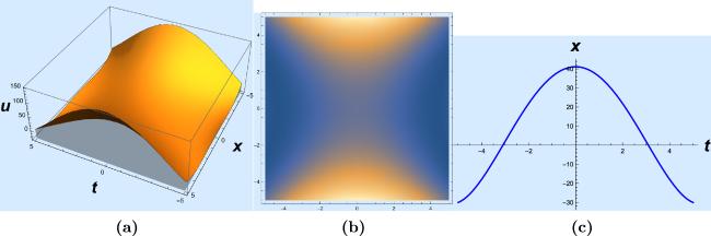
where ${\rho }_{i}$, for $i=0,1$, represent arbitrary constants. The remaining coefficients ${\rho }_{n}$, for $n\geqslant 2$, can be determined iteratively using equations (3.30), (3.31) and (3.32). However, in practical applications, it is often more convenient to work with an approximate form of the solution
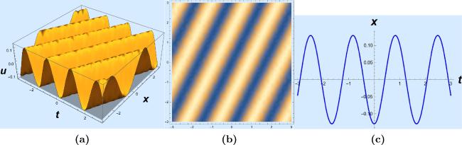
Figure 1. (a) A 3D graph of the bell-shaped solution (3.38) for a = 1, b = 2, ρ0 = 2, ρ1 = 1, and −5 ≤ t, x ≤ 5. (b) A 2D density plot of solution (3.38). (c) A 2D graph of solution (3.38) for x = 3 and −5 ≤ t ≤ 5.
3.4. Solutions of equation (1.3) using the simplest equation approach
We employ the simplest equation approach, as described in [55], to solve the second-order NLODE (2.12). The simplest equations used in this method are the Bernoulli and Riccati equations, given respectively by:
where H(ξ) satisfies either the Bernoulli equation (3.39) or the Riccati equation (3.40), M is a positive integer, determined via the balancing procedure, and A0,…,AM are parameters to be determined. The solutions of the Bernoulli equation (3.39) that we utilize here are
By substituting equation (3.46) into equation (2.12) and utilizing the Bernoulli equation (3.39), we can equate the coefficients of Hi to zero. This leads to a system of four algebraic equations in terms of A0 and A1:
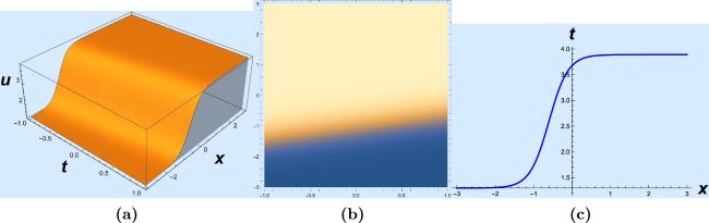
where ξ = x − ct and c0 is an arbitrary constant. The wave profile of the hyperbolic solutions, equations (3.47) and (3.48), can be seen in figures 2 and 3.
Figure 2. (a) A 3D graph of the kink-shaped solution (3.47) for l = 4, b = 2, c = − 0.4, m = 1, c0 = 1, c1 = 1, and −3 ≤ t, x ≤ 3. (b) A 2D density plot of solution (3.47). (c) A 2D graph of solution (3.47) for t = 1 and −3 ≤ x ≤ 3.
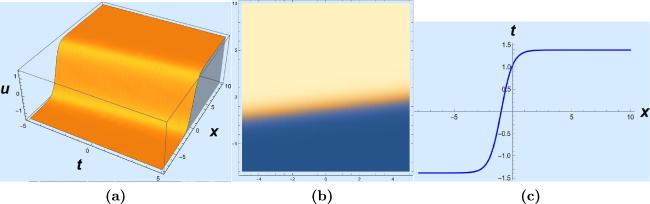
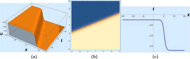
Figure 3. (a) A 3D graph of the kink-shaped solution (3.48) for l = 2, b = 1, c = 0.2, m = 1, c0 = 1, c2 = 1, and −5 ≤ t ≤ 5, −8 ≤ x ≤ 10. (b) A 2D density plot of solution (3.48). (c) A 2D graph of solution (3.48) for t = 0 and −8 ≤ x ≤ 10.
3.4.2. Solutions of equation (1.3) using the Riccati equation
In this case, the balancing procedure gives M = 1 and, therefore, equation (3.41) becomes
Inserting the above expression for G(ξ) into equation (2.12) and making use of the Riccati equation (3.40) yields the following system of four algebraic equations:
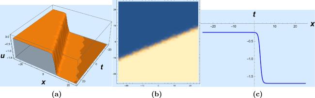
where ξ = x − ct and c0 is an arbitrary constant. The dynamical wave profiles for the solutions, equations (3.50) and (3.51), are shown in figures 4 and 5, respectively.
Figure 4. (a) A 3D graph of the kink-shaped solution (3.50) for l = 4, b = 2, c=0.4, m = 3, n = 1, c0 = 1, c1 = 1, and −25 ≤ t, x ≤ 25. (b) A 2D density plot of solution (3.50). (c) A 2D graph of solution (3.50) for t = 10 and −25 ≤ t ≤ 25.
Figure 5. (a) A 3D graph of the kink-shaped solution (3.51) for l = 4, b = 2, c=0.4, m = 3, n = 1, c0 = 1, c1 = 1, and −15 ≤ t, x ≤ 15. (b) A 2D density plot of solution (3.51). (c) A 2D graph of solution (3.51) for t = 10 and −15 ≤ t ≤ 15.
3.4.3. Solutions of equation (1.3) using the extended Jacobi elliptic function technique
In a similar manner to that discussed in the previous section, our focus now moves towards the acquisition of exact solutions using the extended Jacobi elliptic function expansion method on the NLODE (2.12).
Cnoidal wave solutions of (1.3)
Considering the NLODE (2.12), recall that the balancing procedure leads to M = 1. Thus
where A−1, A0, and A1 are constants that need to be determined. By substituting the above expression for G(ξ) into equation (2.12) and employing equation (3.22), we obtain an equation that can be separated on different powers of G(ξ) and that yields seven distinct algebraic equations
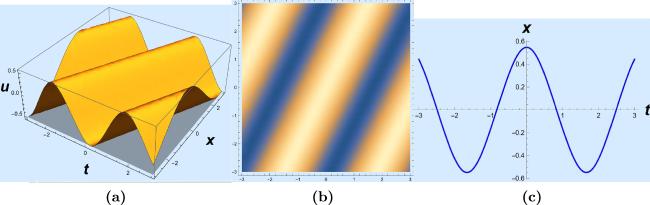
Figure 6. (a) A 3D graph of the periodic soliton solution (3.53) for b = 2, ω = 0.2, c = 2, and −3 ≤ t, x ≤ 3. (b) A 2D density plot of solution (3.53). (c) A 2D graph of solution (3.53) for x = 0 and −3 ≤ t ≤ 3.
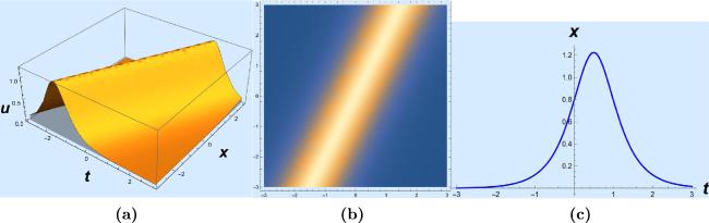
Figure 7. (a) A 3D graph of the bell-shaped soliton solution (3.54) for b = 2, c = 2, and −3 ≤ t, x ≤ 3. (b) A 2D density plot of solution (3.54). (c) A 2D graph of solution (3.54) for x = 1 and −3 ≤ t ≤ 3.
Snoidal wave solutions of equation (1.3)
For the snoidal case, as before, we obtain an equation that can be split into different powers of G(ξ) and that yields seven distinct algebraic equations
respectively. Here, ξ = x − ct. The wave profile of solution (3.55) can be seen in figure 8.
Dnoidal wave solutions of equation (1.3)
In the dnoidal case, we arrive at an equation that can be partitioned into various powers of G(ξ), leading to seven distinct algebraic equations, namely,
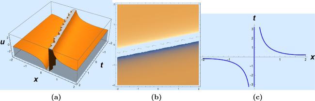
Figure 8. (a) A 3D graph of the singular soliton solution (3.55) for b = 2, ω = 0.5, c = 0.2, and −2 ≤ t, x ≤ 2. (b) A 2D density plot of solution (3.55). (c) A 2D graph of solution (3.55) for t = 0 and −2 ≤ x ≤ 2.
Figure 9. (a) A 3D graph of the periodic soliton solution (3.56) for b = 2, ω = 0.2, c = 2, and −3 ≤ t, x ≤ 3. (b) A 2D density plot of solution (3.56). (c) A 2D graph of solution (3.56) for x = 0 and −3 ≤ t ≤ 3.
Figure 10. (a) A 3D graph of the bell-shaped soliton solution (3.57) for b = 2, c = 2, and −5 ≤ t, x ≤ 5. (b) A 2D density plot of solution (3.57). (c) A 2D graph of solution (3.57) for x = 0 and −5 ≤ t ≤ 5.
4. Conservation laws of the LGHe
Conservation laws delineate physical properties that do not change during several processes that take place in the physical world. These quantities are said to be “conserved”. In physics, for instance, the conserved quantities are energy, momentum, and angular momentum. Here, we attain conserved vectors for the LGHe (1.3) via the engagement of two methods. Firstly, the multiplier approach, as shown in [29], and then, the conservation theorem from Ibragimov, given in [56].
4.1. Conservation laws using the multiplier approach
The multiplier approach is admired for its ability to handle conserved quantities of DEs, whether they possess variational principles or not. We employ the multiplier technique to derive conserved vectors for the LGHe (1.3). It is worth noting that the zeroth-order multiplier yields no results; hence, we shall consider first-order multipliers, namely, Λ = Λ(t, x, u, ut, ux), and use these multipliers to establish the conservation laws of equation (1.3). Recall that the first-order multipliers Λ are determined from the determining equation
By expanding equation (4.58) and following the steps similar to the algorithm for finding the Lie symmetries, we obtain six determining equations, namely,
where Tt is the conserved density and Tx is the spatial flux. Thus, after some tedious computation, the conserved vectors corresponding to the three multipliers are given below.
Case 1. For the first multiplier Λ1 = xut + tux, the corresponding conserved vector is given by
The established method states that each symmetry is associated with a specific conserved quantity [56]. We now use the conservation theorem from Ibragimov to calculate the conserved vectors of the LGHe (1.3). For a more in-depth understanding of the method, the reader can refer to [56].
The adjoint equation for equation (1.3) can be obtained from the formula
which implies that the LGHe is self-adjoint. Considering equation (1.3) and the adjoint equation (4.62) as a system, the formal Lagrangian for this system is
$\begin{eqnarray}{ \mathcal L }=v({u}_{{tt}}-{u}_{{xx}}+{a}^{2}u+{b}^{2}{u}^{3}).\end{eqnarray}$
Recall that the LGHe admits three infinitesimal symmetries. We derive the conserved vectors (Tt, Tx) using the formulae
$\begin{eqnarray}\begin{array}{rcl}{{\boldsymbol{T}}}^{{\boldsymbol{t}}} & = & \tau { \mathcal L }+W\left\{\displaystyle \frac{\partial { \mathcal L }}{\partial {u}_{t}}-{D}_{t}\left(\displaystyle \frac{\partial L}{\partial {u}_{{tt}}}\right)\right\},\\ {{\boldsymbol{T}}}^{{\boldsymbol{x}}} & = & \xi { \mathcal L }+W\left\{\displaystyle \frac{\partial { \mathcal L }}{\partial {u}_{x}}-{D}_{x}\left(\displaystyle \frac{\partial { \mathcal L }}{\partial {u}_{{xx}}}\right)\right\}\\ & & +{W}_{t}\left(\displaystyle \frac{\partial { \mathcal L }}{\partial {u}_{{tt}}}\right),\end{array}\end{eqnarray}$
Case 1. For ${{ \mathcal W }}_{1}=\partial /\partial t$, the Lie characteristic function is given by W1 = − ut. Thus, the conserved vector associated with ${{ \mathcal W }}_{1}$, using equation (4.64), is
Case 2. For the symmetry ${{ \mathcal W }}_{2}=\partial /\partial x$, the Lie characteristic function is W2 = − ux and, consequently, the conserved vector is
Case 3. Finally, for the symmetry ${{ \mathcal W }}_{3}=x\partial /\partial t+t\partial /\partial x$, we have W3 = − (tux + xut). Hence, the corresponding conserved vector is
Remarks. Conservation laws play a pivotal role in the analysis of partial differential equations as they provide conserved quantities for the underlying system. These laws not only enable investigations into integrability and linearization, but also have the potential to yield both qualitative and quantitative insights into the properties of the solutions. Among the conserved vectors derived in this study, we have identified those representing linear momentum and energy. Such conserved quantities hold significant value in the examination of physical systems, as they contribute greatly to the understanding of their dynamics and behaviour. Consequently, these conserved vectors offer a valuable framework for studying the intricacies of physical phenomena. Moreover, the conserved vectors involve solutions u of the LGHe and solutions v of the adjoint equation (4.62) and, hence, yield an infinite number of conserved vectors. Indeed, it is noteworthy that by setting v = u in the conserved vectors derived using Ibragimov’s theorem, we obtain conserved vectors that closely resemble those obtained through the multiplier method. This observation highlights the connection and similarity between the two approaches in identifying and characterizing conserved quantities in the studied system. It suggests that the multiplier method and Ibragimov’s theorem yield consistent results and provide complementary perspectives on the conservation laws governing the system dynamics.
5. Conclusion
This paper has explored the LGHe from a Lie symmetry perspective. The study has presented a comprehensive account of point symmetries admitted by the LGHe. These symmetries have been utilized to perform symmetry reductions, leading to the discovery of group invariant solutions. Various mathematical tools, including Kudryashov’s method, the extended Jacobi elliptic function expansion method, the power series method, and the simplest equation method, have been applied to obtain solutions characterized by exponential, hyperbolic, and elliptic functions. The presence of arbitrary constants in these solutions enhances their significance and applicability in explaining physical phenomena. To visually represent the obtained solutions, Mathematica was employed to generate 3D, 2D, and density plots, as illustrated in figure 1. The plots depict solutions exhibiting kink-shaped, singular kink-shaped, bell-shaped, and periodic patterns. Additionally, the derivation of conserved vectors for the studied model has been accomplished using the multiplier method and Ibragimov’s theorem. This analysis has yielded diverse conserved quantities with practical applications in the field of physical sciences, such as the conservation of energy and momentum. Moreover, among the solutions obtained in this study, only solutions (3.48), (3.50), (3.54), and (3.57) align with the existing literature. However, the remaining solutions are new and novel contributions introduced by this research. Consequently, the newly derived solutions hold potential for further expanding our understanding of the model.
Acknowledgments
M.Y.T. Lephoko would like to thank the South African National Space Agency (SANSA) for funding this work. Additionally, both authors express their gratitude to the Mafikeng campus of North-West University for their ongoing assistance.
Funding
The funding support for this work has been acknowledged.
Conflict of interest
The authors declare that there is no conflict of interest regarding the publication of this paper.
Ethical approval
The authors declare that they have adhered to the ethical standards of research execution.
WazwazA M2009Partial Differential Equations and Solitary Waves Theory Springer
5
AdemA R, KhaliqueC M, MolatiM2015 Group classification, symmetry reductions and exact solutions of a generalized Korteweg–de Vries–Burgers Equation Appl. Math. Inf. Sci.9 501 506
6
SalehM, HassanA A, AltwatyA A2020 Optical solitons of the extended Gerdjikov–Ivanov equation in dwdm system by extended simplest equation method Appl. Math. Inf. Sci.14 901 907
7
AdeyemoO D, KhaliqueC M2021 Symmetry solutions and conserved quantities of an extended (1+3)-dimensional Kadomtsev–Petviashvili-like equation Appl. Math. Inf. Sci.15 649 660
8
ZhangY X, XiaoL N2022 Breather wave and double-periodic soliton solutions for a (2+1)-dimensional generalized Hirota–Satsuma–Ito equation Open Phys.20 632 638
RaoX, ManafianJ, MahmoudK H, HajarA, MahdiA B, ZaidiM2022 The nonlinear vibration and dispersive wave systems with extended homoclinic breather wave solutions Open Phys.20 795 821
DongS H2011Wave Equations in Higher Dimensions Springer
15
DarvishiM T, NajafiM2011 A modification of extended homoclinic test approach to solve the (3+1)-dimensional potential-YTSF equation Chin. Phys. Lett.28 040202
OsmanM S2019 One-soliton shaping and inelastic collision between double solitons in the fifth-order variable-coefficient Sawada–Kotera equation Nonlinear Dyn.96 1491 1496
WazwazA M2007 Traveling wave solution to (2+1)-dimensional nonlinear evolution equations J. Nat. Sci. Math.1 1 13
18
YahyaK H, MoussaZ A2015 New approach of generalized exp (−Φ(η))-expansion method and its application to some nonlinear partial differential equation J. Math. Res.7 106 121
19
GuC H1990Soliton Theory and Its Application Zhejiang Science and Technology Press
20
SalasA H, GomezC A2010 Application of the Cole–Hopf transformation for finding exact solutions to several forms of the seventh-order KdV equation Math. Probl. Eng.2010 194329
WeissJ, TaborM, CarnevaleG1985 The Painlévé property and a partial differential equations with an essential singularity Phys. Lett. A 109 205 208
22
ZhengC L, FangJ P2006 New exact solutions and fractional patterns of generalized Broer–Kaup system via a mapping approach Chaos Soliton Fract.27 1321 1327
ChunC, SakthivelR2010 Homotopy perturbation technique for solving two point boundary value problems-comparison with other methods Comput. Phys. Commun.181 1021 1024
ZengX, WangD S2009 A generalized extended rational expansion method and its application to (1+1)-dimensional dispersive long wave equation Appl. Math. Comput.212 296 304
ZhangL, KhaliqueC M2018 Classification and bifurcation of a class of second-order ODEs and its application to nonlinear PDEs Discrete Contin. Dyn. Syst. -S11 777 790
ChenY, LiB, ZhangH2003 Exact solutions for a new class of nonlinear evolution equations with nonlinear term of any order Chaos Solit. Fractals17 675 682
BekirA, UnsalO2013 Exact solutions for a class of nonlinear wave equations by using first integral method Int. J. Nonlinear Sci.15 99 110
39
BarmanH K, AkbarM A, OsmanM S, NisarK S, ZakaryaM, Abdel-AtyA H, EleuchH2021 Solutions to the Konopelchenko–Dubrovsky equation and the Landau–Ginzburg–Higgs equation via the generalized Kudryashov technique Results Phys.24 104092
IslamM E, AkbarM A2020 Stable wave solutions to the Landau–Ginzburg–Higgs equation and the modified equal width wave equation using the IBSEF method. Arab J. Basic Appl. Sci.27 270 278
KhaliqueC M, AdeyemoO D2023 Lagrangian formulation and solitary wave solutions of a generalized Zakharov–Kuznetsov equation with dual power-law nonlinearity in physical sciences and engineering J. Ocean Eng. Sci.8 152 168
2007Table of Integrals, Series, and ProductsGradshteynI S, RyzhikI M New York Academic 7th edn
49
1964Handbook of Mathematical Functions with Formulas, Graphs and Mathematical TablesAbramowitzM, StegunI A U.S. Government Printing Office
50
FengL, TianS, ZhangT, ZhouJ2017 Lie symmetries, conservation laws and analytical solutions for two-component integrable equations Chinese J. Phys.55 996 1010
Jian-MinT, Shou-FuT, Mei-JuanX, Tian-TianZ2016 On Lie symmetries, optimal systems and explicit solutions to the Kudryashov–Sinelshchikov equation Appl. Math. Comput.275 345 352
53
RudinW2004Principles of Mathematical Analysis 3rd edn China Machine Press
54
FichtenholzG M1970Functional Series Gordon & Breach
55
ZhaoY M, HeY H, LongY2013 The simplest equation method and its application for solving the nonlinear NLSE, KGZ, GDS, DS, and GZ equations J. Appl. Math.2013 960798


