


1. Introduction
There has recently been a great deal of interest both in the theoretical and experimental study of non-Hermitian systems [1–5]. The non-Hermitian systems have been realized in many fields, for example in optics systems [6–9], microwaves systems [10, 11], and electronics systems [12–14]. Projective Hilbert space establishes a bridge between quantum mechanics and modern differential geometry [15, 16], and many important physical quantities, such as Berry curvature [17] and Fisher information [18–20] (the imaginary and real parts of the quantum geometric tensor respectively) are directly related with it. Hence, it plays a crucial role in various aspects of physics, especially in studying geometric and topological properties for quantum systems [21].
The dynamics on the Projective space also play a role in investigating critical behaviors for many quantum systems, for example, the self-trapping in Bose–Einstein condensates [22–24], the non-adiabatic tunneling [25–27], and so on. For non-Hermitian systems, we can also set up the Projective Hilbert space [28–31]. Indeed, for a 2 × 2 matrix Hermitian system, the Projective space is just a Bloch sphere. Hence, it will be interesting to discuss a 2 × 2 matrix non-Hermitian system by employing the Bloch sphere.
In this paper, by introducing the dynamical equations of 2 × 2 matrix non-Hermitian systems on the Bloch sphere, we investigate the dynamical properties of the systems in detail. We find that there are four kinds of fixed points for 2 × 2 matrix non-Hermitian systems, elliptic points, spiral points, critical nodes, and degenerate points. The Hermitian systems and unbroken ${ \mathcal P }{ \mathcal T }$ non-Hermitian cases belong to the category with elliptic points. A system with a degenerate point just corresponds to the system with an exceptional point (EP), namely with an isolated degeneracy. The topology charges of different fixed points are investigated. And, the potential application in two-band systems is also discussed.
The rest of the paper is organized as follows. First, we introduce the definition of the Bloch sphere for non-Hermitian systems in section 2 . Then we investigate the dynamical properties on the Bloch sphere for 2 × 2 matrix non-Hermitian system in section 3 . The cases with EP are discussed in section 4 . In section 5 , we investigate the topological charges of the fixed points. The application in 1D two-band systems is discussed in section 6 . Finally, we give a conclusion of our paper in section 7 .
2. Evolution of the non-Hermitian quantum system on the Bloch sphere
Consider the following Schrödinger equation
$\begin{eqnarray}{\rm{i}}\displaystyle \frac{{\rm{d}}}{{\rm{d}}t}\left(\begin{array}{c}a\\ b\end{array}\right)=\left(\begin{array}{cc}{H}_{11} & {H}_{12}\\ {H}_{21} & {H}_{22}\end{array}\right)\left(\begin{array}{c}a\\ b\end{array}\right),\end{eqnarray}$
where the 2 × 2 matrix H is generally a non-Hermitian Hamiltonian. Let us define ${H}_{11}+{H}_{22}=2{\rm{\Pi }}{{\rm{e}}}^{{\rm{i}}{\eta }_{0}}$, H11 − H22 = 2Ωeiη, ${H}_{12}={\rm{\Gamma }}{{\rm{e}}}^{{\rm{i}}{\delta }_{1}}$, and ${H}_{21}={\rm{\Lambda }}{{\rm{e}}}^{{\rm{i}}{\delta }_{2}}$ for convenience, where Π, Ω, Γ, and Λ are real numbers. The eigenvalues of the system can be easily get $\begin{eqnarray}{E}_{\pm }={\rm{\Pi }}{{\rm{e}}}^{{\rm{i}}{\eta }_{0}}\pm \sqrt{({{\rm{\Omega }}}^{2}{{\rm{e}}}^{2{\rm{i}}\eta }+{\rm{\Gamma }}{\rm{\Lambda }}{{\rm{e}}}^{{\rm{i}}({\delta }_{1}+{\delta }_{2})})}.\end{eqnarray}$
The eigenvalues are a complex pair in general. The complex eigenvalues are in accordance with time evolution not being unitary for non-Hermitian systems. The degeneracy of a non-Hermitian system is a branch-point (commonly called an exceptional point (EP)), at which the two eigenvalues are equal to each other and the eigenstates are parallel [32].The evolution of the non-Hermitian quantum system can be described by the motion on the Bloch sphere [33]. For the system with 2 × 2 matrix H, the vector on the Bloch sphere for a state $| {\rm{\Psi }}\rangle =\left(\begin{array}{c}a\\ b\end{array}\right)$ can be defined as $| \overline{{\rm{\Psi }}}\rangle =\left(\begin{array}{c}| \overline{a}| {{\rm{e}}}^{{\rm{i}}\varphi }\\ | \overline{b}| \end{array}\right)$ with $| {\rm{\Psi }}\rangle ={{\rm{e}}}^{\alpha +{\rm{i}}\beta }| \overline{{\rm{\Psi }}}\rangle $, $\overline{a}=\tfrac{a}{\sqrt{| a{| }^{2}+| b{| }^{2}}}$, $\overline{b}=\tfrac{b}{\sqrt{| a{| }^{2}+| b{| }^{2}}}$, and $\varphi =\arg (a)-\arg (b)$, where α denotes the change in norm factor and β is for total phase shift. By denoting $\,\cos \,\theta =| {\overline{b| }}^{2}-{\overline{| a| }}^{2}$, it then can be mapped to a unit sphere with the spherical coordinates (θ, φ).
Combining with the complex conjugations of equation (1 ), and considering $| \overline{a}{| }^{2}+| \overline{b}{| }^{2}=1$, we obtain the dynamical equation of the system on the Bloch sphere,
$\begin{eqnarray}\begin{array}{l}\displaystyle \frac{{\rm{d}}}{{\rm{d}}t}\varphi =-2{\rm{\Omega }}\,\cos \,\eta +2\left[{\rm{\Lambda }}\,\cos \,(\varphi +{\delta }_{2}){\sin }^{2}\displaystyle \frac{\theta }{2}\right.\\ \left.-\,{\rm{\Gamma }}\,\cos \,(\varphi -{\delta }_{1}){\cos }^{2}\displaystyle \frac{\theta }{2}\right]/\sin \theta ,\end{array}\end{eqnarray}$
$\begin{eqnarray}\begin{array}{l}\displaystyle \frac{{\rm{d}}}{{\rm{d}}t}\theta =2{\rm{\Omega }}\,\sin \,\eta \sin \theta -2\left[{\rm{\Lambda }}\sin (\varphi +{\delta }_{2}){\sin }^{2}\displaystyle \frac{\theta }{2}\right.\\ \left.+\,{\rm{\Gamma }}\sin (\varphi -{\delta }_{1}){\cos }^{2}\displaystyle \frac{\theta }{2}\right],\end{array}\end{eqnarray}$
the changing in norm $\begin{eqnarray}\begin{array}{l}\displaystyle \frac{{\rm{d}}}{{\rm{d}}t}\alpha ={\rm{\Pi }}\sin {\eta }_{0}-{\rm{\Omega }}\sin \eta \,\cos \,\theta +\left[{\rm{\Lambda }}\sin (\varphi +{\delta }_{2})\right.\\ \left.-\,{\rm{\Gamma }}\sin (\varphi -{\delta }_{1})\right]\sin \theta /2,\end{array}\end{eqnarray}$
and the total phase shift $\begin{eqnarray}\displaystyle \frac{{\rm{d}}}{{\rm{d}}t}\beta ={\gamma }_{d}+1/2(1-\,\cos \,\theta )\displaystyle \frac{{\rm{d}}\varphi }{{\rm{d}}t},\end{eqnarray}$
where $\begin{eqnarray}\begin{array}{l}{\gamma }_{d}=-{\rm{\Pi }}\,\cos \,{\eta }_{0}+{\rm{\Omega }}\,\cos \,\eta \,\cos \,\theta -\left[{\rm{\Lambda }}\,\cos \,(\varphi +{\delta }_{2})\right.\\ \left.-{\rm{\Gamma }}\,\cos \,(\varphi -{\delta }_{1})\right]\sin \theta /2\end{array}\end{eqnarray}$
just corresponds to the so-called dynamic phase. The equation of the phase shift is as the same as what had been obtained for Hermitian system by Aharonov and Anandan [34]. The second part in the right hand of the phase shift equation is known as the geometric part.3. Classifying non-Hermitian systems with dynamics on the Bloch sphere
In this section, we will investigate the dynamical behaviors of 2 × 2 non-Hermitian systems in detail based on its Bloch sphere which serves as phase space of the dynamical equations (3 ), (4 )
Letting ${\delta }_{0}=\tfrac{{\delta }_{2}-{\delta }_{1}}{2}$, $\delta =\tfrac{{\delta }_{2}+{\delta }_{1}}{2}$, and φ = φ + δ0 for simplicity, the dynamical equations (3 ), (4 ) can be rewritten as
$\begin{eqnarray}\begin{array}{l}\displaystyle \frac{{\rm{d}}}{{\rm{d}}t}\varphi =-2{\rm{\Omega }}\,\cos \,\eta +2\left[{\rm{\Lambda }}\,\cos \,(\varphi +\delta ){\sin }^{2}\displaystyle \frac{\theta }{2}\right.\\ \left.-\,{\rm{\Gamma }}\,\cos \,(\varphi -\delta ){\cos }^{2}\displaystyle \frac{\theta }{2}\right]/\sin \theta ,\end{array}\end{eqnarray}$
$\begin{eqnarray}\begin{array}{l}\displaystyle \frac{{\rm{d}}}{{\rm{d}}t}\theta =2{\rm{\Omega }}\sin \eta \sin \theta -2\left[{\rm{\Lambda }}\sin (\varphi +\delta ){\sin }^{2}\displaystyle \frac{\theta }{2}\right.\\ \left.+\,{\rm{\Gamma }}\sin (\varphi -\delta ){\cos }^{2}\displaystyle \frac{\theta }{2}\right].\end{array}\end{eqnarray}$
The fixed points are the solutions of the equations $\tfrac{{\rm{d}}}{{\rm{d}}t}\varphi =0$ and $\tfrac{{\rm{d}}}{{\rm{d}}t}\theta =0$, denoted as (φ*, θ*), and they satisfy the following equations,
$\begin{eqnarray}\begin{array}{l}{\rm{\Omega }}\,\cos \,\eta -\left[{\rm{\Lambda }}\,\cos \,({\varphi }^{* }+\delta ){\sin }^{2}\displaystyle \frac{{\theta }^{* }}{2}\right.\\ \left.-\,{\rm{\Gamma }}\,\cos \,({\varphi }^{* }-\delta ){\cos }^{2}\displaystyle \frac{{\theta }^{* }}{2}\right]/\sin {\theta }^{* }=0,\end{array}\end{eqnarray}$
$\begin{eqnarray}\begin{array}{l}{\rm{\Omega }}\sin \eta \sin {\theta }^{* }-\left[{\rm{\Lambda }}\sin ({\varphi }^{* }+\delta ){\sin }^{2}\displaystyle \frac{{\theta }^{* }}{2}\right.\\ \left.+\,{\rm{\Gamma }}\sin ({\varphi }^{* }-\delta ){\cos }^{2}\displaystyle \frac{{\theta }^{* }}{2}\right]=0.\end{array}\end{eqnarray}$
There should be two fixed points in general and related to the eigenstates of the system (1 ) corresponding to the two eigenvalues (2 ) respectively.
A dynamical system may be categorized into different dynamical modes for different parameters by properties of fixed points on phase space. The property of fixed point of phase space is classified by the Jacobian matrix which is obtained by linearizing the dynamical equations around the fixed point [35, 36]. The Jacobian matrix is
$\begin{eqnarray}J=\left(\begin{array}{ll}\displaystyle \frac{\partial }{\partial \varphi }(\dot{\varphi }) & \displaystyle \frac{\partial }{\partial \theta }(\dot{\varphi })\\ \displaystyle \frac{\partial }{\partial \theta }(\dot{\theta }) & \displaystyle \frac{\partial }{\partial \theta }(\dot{\theta })\end{array}\right){\Space{0ex}{2.3ex}{0ex}| }_{({\varphi }^{* },{\theta }^{* })},\end{eqnarray}$
in which $\dot{x}$ means $\tfrac{{\rm{d}}x}{{\rm{d}}t}$.From the equations (8 ) and (9 ), the elements of the Jacobian matrix can be derived as follows
$\begin{eqnarray}\begin{array}{l}{J}_{11}=-2\left[{\rm{\Lambda }}\sin ({\varphi }^{* }+\delta ){\sin }^{2}\displaystyle \frac{{\theta }^{* }}{2}\right.\\ \left.-\,{\rm{\Gamma }}\sin ({\varphi }^{* }-\delta ){\cos }^{2}\displaystyle \frac{{\theta }^{* }}{2}\right]/\sin {\theta }^{* },\end{array}\end{eqnarray}$
$\begin{eqnarray}\begin{array}{l}{J}_{12}=\left[{\rm{\Lambda }}\,\cos \,({\varphi }^{* }+\delta )\right.\\ \left.+\,{\rm{\Gamma }}\,\cos \,({\varphi }^{* }-\delta )\right]-2{\rm{\Omega }}\,\cos \,\eta \,\cos \,\theta /\sin {\theta }^{* },\end{array}\end{eqnarray}$
$\begin{eqnarray}\begin{array}{l}{J}_{21}=-2\left[{\rm{\Lambda }}\,\cos \,({\varphi }^{* }+\delta ){\sin }^{2}\displaystyle \frac{{\theta }^{* }}{2}\right.\\ \left.+\,{\rm{\Gamma }}\,\cos \,({\varphi }^{* }-\delta ){\cos }^{2}\displaystyle \frac{{\theta }^{* }}{2}\right],\end{array}\end{eqnarray}$
$\begin{eqnarray}\begin{array}{l}{J}_{22}=-\left[{\rm{\Lambda }}\sin ({\varphi }^{* }+\delta )\right.\\ \left.-\,{\rm{\Gamma }}\sin ({\varphi }^{* }-\delta )\right]\sin {\theta }^{* }+2{\rm{\Omega }}\sin \eta \,\cos \,{\theta }^{* }.\end{array}\end{eqnarray}$
By taking the equations of fixed point (10 ) and (11 ) into account, we can have
$\begin{eqnarray}{J}_{11}={J}_{22},\quad {J}_{12}=-{J}_{21}/{\sin }^{2}{\theta }^{* }.\end{eqnarray}$
For simplicity, we define $\begin{eqnarray}{J}_{1}={J}_{11}\sin {\theta }^{* },\quad {J}_{2}={J}_{21}.\end{eqnarray}$
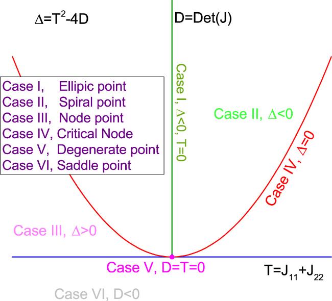
Figure 1. The category of the fixed points, classified by trace and determinant of Jacobian matrix J defined in equation ( |
In fact, for different parameter regions in figure 1, the eigenvalues ${\lambda }_{\pm }=-T/2\pm \sqrt{{\rm{\Delta }}}/2$ of the Jacobian are different. For case I, the λ± are a pure imaginary pair; for case II, λ± are a complex pair; for case III, there are two negative real eigenvalues; for case IV, there is only one nonzero real eigenvalue, i.e. λ+ = λ− = − T/2, while for case V the eigenvalues are zeros; for case VI, there are two real eigenvalues with λ+ > 0 > λ−.
For a 2 × 2 non-Hermitian system, from (17 ), we get $D=({J}_{1}^{2}+{J}_{2}^{2})/{\sin }^{2}{\theta }^{* }$, and then we can obtain ${\rm{\Delta }}=-4{J}_{2}^{2}/{\sin }^{2}{\theta }^{* }$. Hence, for the system Δ ≤ 0, we can immediately know that there are no saddle points and node points for a 2 × 2 non-Hermitian system.
We then have four kinds of dynamical modes, a) T = 0, Δ < 0, the system belonging to Case I. b) T ≠ 0, Δ ≠ 0, the system belonging to Case II. c) T ≠ 0, Δ = 0, the system belonging to Case IV. And d) T = Δ = 0, the system belonging to Case V.
For mode a), because T = 0 and Δ ≠ 0, we easily have J1 = 0, J2 ≠ 0. Combining with the fixed point equations (10 ) and (11 ), we can get
$\begin{eqnarray}{J}_{2}^{2}-{J}_{1}^{2}=4{{\rm{\Omega }}}^{2}\cos 2\eta +4{\rm{\Lambda }}{\rm{\Gamma }}\cos 2\delta ,\end{eqnarray}$
$\begin{eqnarray}{J}_{1}{J}_{2}=2{{\rm{\Omega }}}^{2}\sin 2\eta +2{\rm{\Lambda }}{\rm{\Gamma }}\sin 2\delta .\end{eqnarray}$
Taking equation (2 ) into account, we can find that the energy gap, Eg = E+ − E−, has the following form
$\begin{eqnarray}{E}_{g}=\displaystyle \frac{{J}_{2}+{\rm{i}}{J}_{1}}{2}.\end{eqnarray}$
Then, we have Eg = J2/2 which is a real number. Hence, if the fixed point is an elliptic point, it means that the system will have a real energy gap. The Hermitian systems and ${ \mathcal P }{ \mathcal T }$ unbroken systems all belong to this kind. We plot the trajectories in phase space in figure 2(a) with a set of parameters satisfying T = 0 as an example.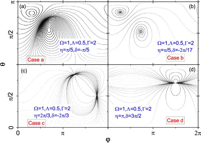
Figure 2. The trajectories in the phase space examples for different cases. (a) For dynamical mode a, (b) for mode b, (c) for mode c, and (d) for mode c. |
For mode b), T ≠ 0, Δ ≠ 0, then J1 ≠ 0, J2 ≠ 0. The system belongs to case II and the fixed points are spirals. For T > 0, the trajectories around it spiral outwards, while for T < 0 they spiral inwards. Eg is a complex number for this case. An example for such a case is plotted in figure 2(b).
For mode c), T ≠ 0, Δ = 0, and J1 ≠ 0 but J2 = 0. The system belongs to Case IV and the fixed points are critical nodes. For T > 0, it is a source, while for T < 0 it is a sink. Eg = iJ1/2 is a pure imaginary number. There is an example for such a case in figure 2(c). The ${ \mathcal P }{ \mathcal T }$ broken systems belong to this kind, of which Λ = Γ, δ1 = − δ2, and η = π/2.
The mode d) is for high order critical point with a zero Jacobian matrix J = 0 and the gap Eg is also zero, which just corresponds to EP. An example for this case is shown in figure 2(d), in which there is only one fixed point since the two eigenstates coalesce together for EP. We will give more discussions for this case in the following since the EP plays an important role in a non-Hermitian system.
The above discussions show that the categories of the fixed points are related to the eigenvalues of the Jacobian matrix which is known as ${\lambda }_{\pm }=-({J}_{1}+{J}_{2})/2\pm {\rm{i}}{J}_{2}/2\sin {\theta }^{* }$ and also with the energy gap of the non-Hermitian system. We summarize the properties in table 1.
Table 1. Summary of the properties of the fixed points for a 2 × 2 non-Hermitian system. Here, PI means pure imaginary. |
| Case | a | b | c | d |
|---|---|---|---|---|
| λ | PI | Complex | Real | Zero |
| Energy gap | Real | Complex | PI | Zero |
| Category | Elliptic | Spiral | Node | Coalesced |
4. The dynamics on the Bloch sphere for systems with EP
The EP means a kind of degeneracy which only appear in a non-Hermitian system [32], and the degeneracies also happen for eigenstates so that there is only one fixed point for such a case. The system with an EP has zero gap and zero Jacobian matrix as we know, and for which the parameters satisfy10 ) and (11 ), we can easily get
$\begin{eqnarray}{{\rm{\Omega }}}^{2}={\rm{\Lambda }}{\rm{\Gamma }},\quad \delta =\eta \pm \displaystyle \frac{\pi }{2}.\end{eqnarray}$
Then, from the equations of fixed point ( $\begin{eqnarray}{\theta }^{* }=2\mathrm{arc}\cot (\sqrt{{\rm{\Lambda }}/{\rm{\Gamma }}}),\quad {\varphi }^{* }=\eta -\delta .\end{eqnarray}$
Obviously, the coordinate θ* for an EP is determined by two parameters among Ω, Λ, and Γ, and φ* is determined by the relation of η and δ.In figure 3, we plot the trajectories in phase space with EP for different η but fixed parameters Ω, Λ, and Γ and the relation δ = η − π/2. One can find that the degenerate point is fixed but the dynamic behaviors are quite different for different η. At the fixed point, all the trajectories are tangent, but the tangent direction changes with η.
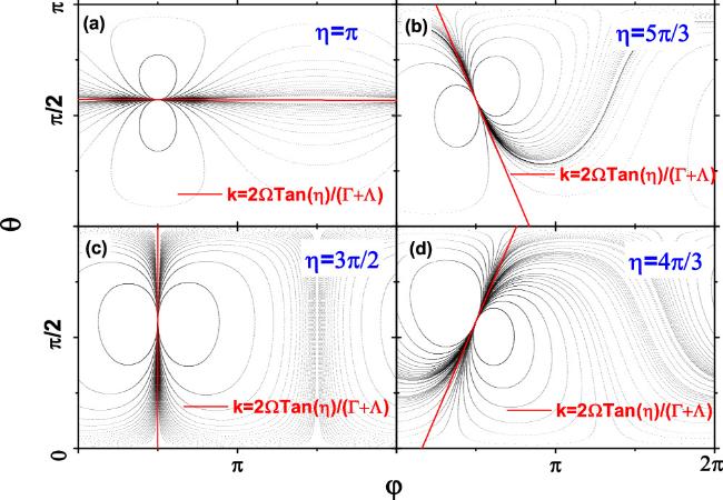
Figure 3. The trajectories in phase space for cases with EP. The parameters are Γ = 0.8, Λ = 1.25, and Ω = 1. $\delta =\eta -\tfrac{\pi }{2}$ with (a) for η = π, (b) for η = 2π/3, (c) for η = π/2, and (d) for η = π/3. |
In order to investigate the dynamics around the fixed point with EP, we need to expand the dynamic equations (8 ), (9 ) around the fixed point to 2th order terms of δθ = θ − θ* and δφ = φ − φ*, since the first order terms are zero. The expansions can be written as
$\begin{eqnarray}\displaystyle \frac{{\rm{d}}\delta \varphi }{{\rm{d}}{t}}={A}_{1}\delta {\varphi }^{2}+{A}_{2}\delta \theta \delta \varphi +{A}_{3}\delta {\theta }^{2},\end{eqnarray}$
$\begin{eqnarray}\displaystyle \frac{{\rm{d}}\delta \theta }{{\rm{d}}{t}}={B}_{1}\delta {\varphi }^{2}+{B}_{2}\delta \theta \delta \varphi +{B}_{3}\delta {\theta }^{2}.\end{eqnarray}$
Here, $\begin{eqnarray}{A}_{1}=-({\rm{\Gamma }}+{\rm{\Lambda }})\,\cos \,\eta \sin {\theta }^{* },\end{eqnarray}$
$\begin{eqnarray}{A}_{2}=-2({\rm{\Gamma }}+{\rm{\Lambda }})\sin \eta ,\end{eqnarray}$
$\begin{eqnarray}{A}_{3}=({\rm{\Gamma }}+{\rm{\Lambda }})\,\cos \,\eta /\sin {\theta }^{* },\end{eqnarray}$
and $\begin{eqnarray}{B}_{1}=({\rm{\Gamma }}+{\rm{\Lambda }})\sin \eta {\sin }^{2}{\theta }^{* },\end{eqnarray}$
$\begin{eqnarray}{B}_{2}=-2({\rm{\Gamma }}+{\rm{\Lambda }})\,\cos \,\eta \sin {\theta }^{* },\end{eqnarray}$
$\begin{eqnarray}{B}_{3}=-({\rm{\Gamma }}+{\rm{\Lambda }})\sin \eta {\cos }^{2}{\theta }^{* }-2{\rm{\Omega }}\sin \eta \sin {\theta }^{* }.\end{eqnarray}$
Let us define k = δθ/δφ, and substitute it into equations (24 ), (25 ). Then from equations (24 ), (25 ), we can obtain
$\begin{eqnarray}k=2{\rm{\Omega }}/({\rm{\Gamma }}+{\rm{\Lambda }})\tan \eta .\end{eqnarray}$
In figure 3, we plot the lines δθ = kδφ in red dashed lines for different η, which are consistent with the tangent of trajectories at the fixed point for EP.5. Topological charge of fixed points
We can associate a topological charge to the fixed point. Let us introduce a vector field v = (vφ, vθ) with ${v}_{\varphi }=\tfrac{{\rm{d}}\varphi }{{\rm{d}}t}$ and ${v}_{\theta }=\tfrac{{\rm{d}}\theta }{{\rm{d}}{t}}$. This vector just corresponds to tangent vector of the trajectory in phase space. Obviously, in terms of v, a fixed point is just for v = 0.
Then, we define a unit vector field n = v/v = (nφ, nθ) with $v=\sqrt{{v}_{\varphi }^{2}+{v}_{\theta }^{2}}$. Considering a simple closed curve C in phase space, we define the topological charge with
$\begin{eqnarray}w=\displaystyle \frac{1}{2\pi }{\oint }_{C}{A}_{\mu }{\rm{d}}\mu ,\quad \mu =(\theta ,\varphi )\end{eqnarray}$
in which, Aμ = nφ∂μnθ − ∂μnφnθ. [38]In fact, if we parameterize the vector v = (vφ, vθ) via an angle Θ with ${v}_{\varphi }=v\,\cos \,{\rm{\Theta }}$ and ${v}_{\theta }=v\sin {\rm{\Theta }}$, the path integral of equation (33 ) will become $w=\tfrac{1}{2\pi }{\oint }_{C}{\rm{d}}{\rm{\Theta }}$, and $w\in {\mathbb{Z}}$ is the winding number of v [39]. The integer w is just the topological charge of a fixed point.
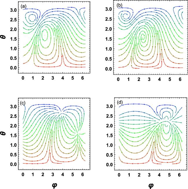
Through calculations, we find that for an elliptic point, a spiral point, and a critical node, the topological charge is w = 1 respectively, while for the degenerate point with an EP, the charge is w = 2. The results can be understood intuitively. In figure 4, we plot the vector streams of the unit vector n = (nφ, nθ) in phase space for different cases. One can see that the vector n = (nφ, nθ) rotates clockwise at a 2π angle when a closed path circulates clockwise which encloses an elliptic point, a spiral point, or a critical node. For the system with an EP, the vector winds twice clockwise when a closed path circulates clockwise which encloses the fixed point.
Figure 4. The vector streams of n = (nφ, nθ) in phase space for cases with the same parameters in figure 2 respectively. |
The total topological charge for the phase space, the sum of the charge of the fixed points is 2 for all cases, which is determined by the topology of a sphere. We know that the sum of the topological indices of the zero points of a tangent vector field is a topological invariant, the Euler number, which is 2 for a sphere [36, 40].
6. Two-band non-Hermitian systems
The above discussion can be used in investigating 1D two-band systems, which can be generally described by
$\begin{eqnarray}H(k)=\displaystyle \sum _{i=1}^{3}({v}_{i}(k)+{\rm{i}}{g}_{i}){\sigma }_{i},\end{eqnarray}$
where σi, (i = 1, 2, 3) are the three pauli matrices, vi(k) and gi are real numbers [41].Comparing with equation (1 ), we have Π = η0 = 0, ${\rm{\Omega }}(k)$$=\sqrt{{v}_{3}{\left(k\right)}^{2}+{g}_{3}^{2}}$, $\eta (k) =\arctan [{g}_{3}/{v}_{3}(k)]$, ${\rm{\Gamma }}(k)= \sqrt{{\left({v}_{1}(k)+{g}_{2}\right)}^{2}+({g}_{1}\,-\, {v}_{2}{\left(k,)\right)}^{2}},{\delta }_{1}(k)$=$\arctan [({g}_{1}$-${v}_{2}(k))/({v}_{1}(k)+{g}_{2})]$, ${\rm{\Lambda }}(k)$$=\sqrt{{\left({v}_{1}(k)-{g}_{2}\right)}^{2}+({g}_{1}+{v}_{2}{\left(k,)\right)}^{2}}$, and ${\delta }_{2}(k)$ $=\arctan [({g}_{1}+{v}_{2}(k))$$/({v}_{1}(k)-{g}_{2})]$.
For example, if ${v}_{1}={t}_{a}+{t}_{b}\cos k,{v}_{2}={t}_{b}\sin k,{v}_{3}=0$, and g1 = g2 = 0, one gets a ${ \mathcal P }{ \mathcal T }$-symmetric Su–Schrieffer–Heeger (SSH) model described by [42].
7. Conclusion
In the above, we show that the dynamics of 2 × 2 non-Hermitian systems can be divided into four different categories with the properties of the fixed points in phase space (Bloch sphere serving as phase space). The different kind of fixed point corresponds to the system that has the different energy gap. Especially, for systems with elliptic points, the gap is real, while for a degenerate point, the gap is zero and the system has an EP. The topological properties of the fixed points have also been investigated. The evolutions of the norm and the total phase have not been studied in this paper. We can know that for the fixed point, the norm will increase or decrease exponentially with a constant exponential factor, hence the norm will be infinitely large or infinitely small asymptotically with time. The total phase will change at a constant rate.