


1. Introduction
The thermodynamic and transport properties of non-Fermi liquids such as high temperature cuprate superconductors strongly differ from those described by the standard Fermi liquid theory [1]. There is still no satisfactory theoretical framework to describe them so far. The AdS/CFT correspondence, also known as holographic duality [2–4], provides a useful tool for high-Tc cuprate strange metals and other strongly correlated systems [5–7]. Recently, holographic duality has brought some new breakthroughs and discussions in condensed matter physics, such as: holographic superconductivity model [8–11], strange metal [12, 13], linear resistivity [14, 15], and Hall angle [16, 17].
There are some similarities in the temperature-doped phase diagrams of many unconventional superconductors, such as high temperature cuprates [9, 18, 19], with an antiferromagnetic phase, a superconducting phase, a metallic phase and a striped phase competing and co-existing with each other. The question of how to construct a holographic theoretical model to reproduce and understand such a phase diagram becomes an important problem. In recent years, holographic two-current models have attracted some attention [20–27]. It has been pointed out that the model has a corresponding Mott insulator [28–31], and there are two spintronic ‘up’ and ‘down’ currents which can be regarded as independent entities at low temperatures [25, 32, 33]. These models include two gauge fields in bulk describing the two currents of the dual boundary field theory. Two independent conserved currents are associated with two different chemical potentials or charged densities, and their ratio defines the ‘doping’ variable x, i.e. x = ρA/ρB. Recently, Kiritsis et al [21] added the related bulk fields dual to the operators of the boundary field theory to simulate the phase diagram that the normal phase, superconducting phase, antiferromagnetic phase and fringe phase compete with each other and co-exist in the temperature-doped plane, in which the superconducting phase appears in the dome-shaped region in the middle of the phase plane. [22] introduces a neutral axion field of [34] to break the translational symmetry of the system, so that the normal phase has a finite DC conductivity distinguished from the superconducting phase. Their results also demonstrate that Kiritsis’ superconducting dome still exists even with broken translational symmetry. Subsequent studies use this model to discuss the effects of quantum critical points on the dome under hyperscaling violation geometry [23]. They reconsidered the role of the first class of charges with density ρA in the temperature-doping phase diagram to form the Mott insulator, and the second class of charges with density ρB to form additional charges by doping.
On the other hand, previous studies construct holographic models with hyperscaling violating factor [35, 36]. In particular, the Gubser–Rocha model is characterized by the dynamical critical exponent z → ∞ and hyperscaling violating exponent θ → − ∞ . It implies the entropy is proportional to near zero temperature with local quantum criticality [37, 38]. It is similar to more realistic strange metals [39, 40]. In order to simulate a more realistic holographic superconductor, we construct a holographic superconducting dome in the Gubser–Rocha model with two charges. One kind of charge is non-movable, which contributes to the half filled state of the Mott insulator. One kind of charge is movable, which contributes to the state near the Fermi surface. The ratio of these two charges is the doping parameter. When the ratio increases, there is a dome-shaped superconducting region which is experimentally observed. That is, the critical temperature rises first and then decreases with the increase of doping. In order to make the conductivity realistic, we also introduce a holographic superconductor with momentum dissipation by breaking translational symmetry [34, 41, 42]. By calculating the DC conductivity of our model, we prove that the normal phase of the model satisfies the linear-T resistivity relation [14] in the presence of momentum dissipation. We also numerically calculate the AC conductivity [43–45] of the normal phase with momentum dissipation. We also calculate spin conductivity γ of our model, and as a result we observe behavior similar to the conductivity of the Mott insulators. We see that there is indeed a superconducting dome phase in the middle of the x-T plane in the Gubser–Rocha model, and unlike previous results, its profile shrinks inward at near zero temperature.
This paper is organized as follows. In section 2 , we set up the doped holographic superconductor, based on the Gubser–Rocha model with broken translational symmetry. In section 3 , we obtain the linear-T resistivity analytically and AC conductivities numerically in the normal phase in order to explore the two-current model. In section 4 , the normal phase of the bulk system was observed to become unstable at Tc, then developing a non-trivial profile of the scalar field χ, which means a superconducting phase transition. We study superconducting instability with the critical temperature Tc by numerically solving the motion equation of χ in the normal phase background, and draw the superconducting dome phase in a temperature-doping plane. We conclude with discussions in section 5 .
2. Construction of the doped superconductor in the Gubser–Rocha model
Inspired by [22], we try to construct a holographic superconducting dome in the Gubser–Rocha model [37]. We consider the following action (1 ):
$\begin{eqnarray}\begin{array}{rcl}S & = & \displaystyle \int \sqrt{-g}\left[{ \mathcal R }+\displaystyle \frac{6}{{L}^{2}}\cosh \varphi -\displaystyle \frac{1}{4}\left({{\rm{e}}}^{\varphi }+{Z}_{A}(\chi )\right){A}_{\mu \nu }{A}^{\mu \nu }\right.\\ & & -\ \displaystyle \frac{1}{4}\left({{\rm{e}}}^{\varphi }+{Z}_{B}(\chi )\right){B}_{\mu \nu }{B}^{\mu \nu }-\displaystyle \frac{1}{2}{Z}_{{AB}}(\chi ){A}_{\mu \nu }{B}^{\mu \nu }\\ & & -\ \displaystyle \frac{3}{2}{\left({\partial }_{\mu }\varphi \right)}^{2}-H(\chi ){\left({\partial }_{\mu }\theta -{q}_{A}{A}_{\mu }-{q}_{B}{B}_{\mu }\right)}^{2}-{V}_{\mathrm{int}}(\chi )\\ & & -\ \left.{{\rm{\Sigma }}}_{I=x,y}{\left(\partial {\phi }_{I}\right)}^{2}-\displaystyle \frac{1}{2}{\left({\partial }_{\mu }\chi \right)}^{2}\right]{{\rm{d}}}^{4}x,\end{array}\end{eqnarray}$
where we set the gravitational constant 16πG = 1. The scalar field φ is the dilaton that makes the entropy proportional to the near zero temperature. The Aμν and Bμν stand for the field strengths of the gauge fields Aμ and Bμ which provide the finite chemical potentials. We introduce a perturbative charge complex scalar ψ = χeiθ for superconducting instability, χ and θ are the amplitude and phase of the charged complex scalar field, respectively. ZA, ZB and ZAB are non-trivial coupling, and Vint is the potential term for the scalar field. We will fix these terms later. The two axions φI: φx = mx, φy = my break the translational invariance.The corresponding equations of motion with the action (1 ) are obtained, as follows. The scalar field χ 's equation is
$\begin{eqnarray}\begin{array}{l}{{\rm{\nabla }}}_{\mu }{{\rm{\nabla }}}^{\mu }\chi -{\partial }_{\chi }{V}_{{\rm{int}}}(\chi )\\ \ \ -\ \displaystyle \frac{1}{4}{\partial }_{\chi }{Z}_{A}(\chi ){A}^{2}-\displaystyle \frac{1}{4}{\partial }_{\chi }{Z}_{B}(\chi ){B}^{2}-\displaystyle \frac{1}{2}{\partial }_{\chi }{Z}_{{AB}}(\chi ){A}_{\mu \nu }{B}^{\mu \nu }\\ \ \ -\ {\partial }_{\chi }H(\chi ){\left({\partial }_{\mu }\theta -{q}_{A}{A}_{\mu }-{q}_{B}{B}_{\mu }\right)}^{2}=0.\end{array}\end{eqnarray}$
The equations of motion of the other matter fields are $\begin{eqnarray}3{{\rm{\nabla }}}_{\mu }{{\rm{\nabla }}}^{\mu }\varphi +\displaystyle \frac{6}{{L}^{2}}\sinh \varphi -\displaystyle \frac{1}{4}{{\rm{e}}}^{\varphi }{A}^{2}-\displaystyle \frac{1}{4}{{\rm{e}}}^{\varphi }{B}^{2}=0,\end{eqnarray}$
$\begin{eqnarray}\begin{array}{l}{{\rm{\nabla }}}_{\mu }\left[\left({{\rm{e}}}^{\varphi }+{Z}_{A}\right){A}^{\mu \nu }\right]+{{\rm{\nabla }}}_{\mu }\left[\left({{\rm{e}}}^{\varphi }+{Z}_{{AB}}\right){B}^{\mu \nu }\right]\\ +\ 2{q}_{A}H(\chi )\left({\partial }^{\nu }\theta -{q}_{A}{A}^{\nu }-{q}_{B}{B}^{\nu }\right)=0,\end{array}\end{eqnarray}$
$\begin{eqnarray}\begin{array}{l}{{\rm{\nabla }}}_{\mu }\left[\left({{\rm{e}}}^{\varphi }+{Z}_{B}\right){B}^{\mu \nu }\right]+{{\rm{\nabla }}}_{\mu }\left[\left({{\rm{e}}}^{\varphi }+{Z}_{{AB}}\right){A}^{\mu \nu }\right]\\ +\ 2{q}_{B}H(\chi )\left({\partial }^{\nu }\theta -{q}_{A}{A}^{\nu }-{q}_{B}{B}^{\nu }\right)=0,\end{array}\end{eqnarray}$
and ∇μ∇μφI = 0 for the axions. The Einsteins equation is given by $\begin{eqnarray}\begin{array}{l}{{ \mathcal R }}_{\mu \nu }-\displaystyle \frac{1}{2}\left({{\rm{e}}}^{\varphi }+{Z}_{A}\right){A}_{\mu }^{\,\beta }{A}_{\nu \beta }-\displaystyle \frac{1}{2}\left({{\rm{e}}}^{\varphi }+{Z}_{B}\right){B}_{\mu }^{\,\beta }{B}_{\nu \beta }\\ -\ \displaystyle \frac{1}{2}{Z}_{{AB}}\left({g}^{\alpha \beta }{A}_{\mu \beta }{B}_{\nu \alpha }+{g}^{\alpha \beta }{B}_{\mu \beta }{A}_{\nu \alpha }\right)\\ -\ \displaystyle \frac{1}{2}{\partial }_{\mu }\chi {\partial }_{\nu }\chi -H(\chi )\left({\partial }_{\mu }\theta -{q}_{A}{A}_{\mu }-{q}_{B}{B}_{\mu }\right)\\ \ \ \times \ \left({\partial }_{\nu }\theta -{q}_{A}{A}_{\nu }-{q}_{B}{B}_{\nu }\right)\\ -\ \displaystyle \frac{3}{2}{\partial }_{\mu }\varphi {\partial }_{\nu }\varphi -\displaystyle \sum _{I=x,y}{\partial }_{\mu }{\phi }_{I}{\partial }_{\nu }{\phi }_{I}\\ -\ \displaystyle \frac{1}{2}{g}_{\mu \nu }\left[{ \mathcal R }+\displaystyle \frac{6}{{L}^{2}}\cosh \varphi -\displaystyle \frac{1}{4}\left({{\rm{e}}}^{\varphi }+{Z}_{A}(\chi )\right){A}_{\mu \nu }{A}^{\mu \nu }\right.\\ -\ \displaystyle \frac{1}{4}\left({{\rm{e}}}^{\varphi }+{Z}_{B}(\chi )\right){B}_{\mu \nu }{B}^{\mu \nu }-\displaystyle \frac{1}{2}{Z}_{{AB}}(\chi ){A}_{\mu \nu }{B}^{\mu \nu }\\ -\ \displaystyle \frac{3}{2}{\left({\partial }_{\mu }\varphi \right)}^{2}-H(\chi ){\left({\partial }_{\mu }\theta -{q}_{A}{A}_{\mu }-{q}_{B}{B}_{\mu }\right)}^{2}-{V}_{{int}}(\chi )\\ \left.-\ {{\rm{\Sigma }}}_{I=x,y}{\left(\partial {\phi }_{I}\right)}^{2}-\displaystyle \frac{1}{2}{\left({\partial }_{\mu }\chi \right)}^{2}\right]=0.\end{array}\end{eqnarray}$
In the following part, the couplings and potential are considered as: $\begin{eqnarray}\begin{array}{l}{Z}_{A}(\chi )=\displaystyle \frac{a{\chi }^{2}}{2},\,\,{Z}_{B}(\chi )=\displaystyle \frac{b{\chi }^{2}}{2},\,\,{Z}_{{AB}}(\chi )=\displaystyle \frac{c{\chi }^{2}}{2},\,\\ H(\chi )=\displaystyle \frac{n{\chi }^{2}}{2},\,\,{V}_{\mathrm{int}}(\chi )=\displaystyle \frac{{M}^{2}{\chi }^{2}}{2}.\end{array}\end{eqnarray}$
And we define the U(1)A,B charges to be: $\begin{eqnarray}{q}_{A}=1,\,\,\,\,\,\,{q}_{B}=0.\end{eqnarray}$
Although this value is very specific, Kiritsis et al have verified that this is feasible [21].To obtain the solutions for this holographic system (1 ), we assume the metric ansatz
$\begin{eqnarray}\begin{array}{l}{\rm{d}}{s}^{2}=-f(r){\rm{d}}{t}^{2}+\displaystyle \frac{{\rm{d}}{r}^{2}}{f(r)}+g(r)\left({\rm{d}}{x}^{2}+{\rm{d}}{y}^{2}\right),\\ {A}_{t}={A}_{t}(r),\,\,\,{B}_{t}={B}_{t}(r),\\ {\phi }_{x}={mx},\,\,\,\,{\phi }_{y}={my},\\ \varphi =\varphi (r),\,\,\,\,\chi =\chi (r),\,\,\,\,\theta \equiv 0,\end{array}\end{eqnarray}$
where x, y are spatial coordinates on the boundary and r denotes the radial bulk coordinate. The boundary is located at r → ∞ , the horizon is located at r = r0. The Hawking temperature of the black brane is given by $\begin{eqnarray}T={\left.\displaystyle \frac{{f}^{{\prime} }(r)}{4\pi }\right|}_{{r}_{0}}.\end{eqnarray}$
In normal phase (χ ≡ 0), our model admits the following solution,
$\begin{eqnarray}\begin{array}{l}\varphi (r)=\displaystyle \frac{1}{2}\mathrm{ln}(1+Q/r),\,\,g(r)={r}^{1/2}{\left(r+Q\right)}^{3/2},\,\,\\ f(r)={r}^{1/2}{\left(r+Q\right)}^{3/2}(1-\displaystyle \frac{({\mu }^{2}+{\mu }_{B}^{2}){\left(Q+{r}_{0}\right)}^{2}}{3Q{\left(r+Q\right)}^{3}}-\displaystyle \frac{{m}^{2}}{{\left(r+Q\right)}^{2}}).\\ {A}_{t}(r)=\mu (1-\displaystyle \frac{{r}_{0}+Q}{r+Q}),\,\,\,{B}_{t}(r)={\mu }_{B}(1-\displaystyle \frac{{r}_{0}+Q}{r+Q}),\\ {\phi }_{x}={mx},\,\,\,{\phi }_{y}={my},\end{array}\end{eqnarray}$
where r0 denotes the horizon radius, m denotes a strength of the momentum relaxation, Q is a physical parameter. The density of the charge carriers is denoted by ρA = μ(Q + r0), which is dual to the gauge field Aμ, while the density of the doped charge ρB = μB(Q + r0) is dual to the gauge field Bμ. The doping ratio is given by: $\begin{eqnarray}{\rm{x}}=\displaystyle \frac{{\rho }_{B}}{{\rho }_{A}}=\displaystyle \frac{{\mu }_{B}}{\mu }.\end{eqnarray}$
The chemical potentials μ and μB satisfy the following equations, $\begin{eqnarray}\mu =\sqrt{\displaystyle \frac{3Q(Q+{r}_{0})}{1+{{\rm{x}}}^{2}}\left(1-\displaystyle \frac{{m}^{2}}{{\left(Q+{r}_{0}\right)}^{2}}\right)},\end{eqnarray}$
$\begin{eqnarray}{\mu }_{B}={\rm{x}}\sqrt{\displaystyle \frac{3Q(Q+{r}_{0})}{1+{{\rm{x}}}^{2}}\left(1-\displaystyle \frac{{m}^{2}}{{\left(Q+{r}_{0}\right)}^{2}}\right)}.\end{eqnarray}$
The Hawking temperature is given by $\begin{eqnarray}T={r}_{0}^{\tfrac{1}{2}}\displaystyle \frac{\left(3{\left(Q+{r}_{0}\right)}^{2}-{m}^{2}\right)}{4\pi {\left(Q+{r}_{0}\right)}^{\tfrac{3}{2}}}.\end{eqnarray}$
3. Conductivities in the normal phase
We consider the momentum dissipation and calculate AC/DC conductivities of our model in the normal phase. Due to the symmetry of the x-y plane, without loss of generality, we only consider the disturbance in the x direction. The system includes two U(1) fields A and B as whose dual operators in the boundary theory denoted as JA and JB describing two currents, respectively. We also write corresponding external electric fields and conductivities as EA, EB and σA, σB, respectively. In general, the external field EA also contributes to the current JB. This process is reciprocal. The associated conductivity is called as γ. σA and σB are interpreted as electric conductivity and spin-spin conductivity, and relatively γ is spin conductivity [26]. The heat current ${ \mathcal Q }$ is also coupled with these two currents. They satisfy Ohm’s law, which is expressed as
$\begin{eqnarray}\left(\begin{array}{c}{J}_{A}\\ { \mathcal Q }\\ {J}_{B}\end{array}\right)=\left(\begin{array}{ccc}{\sigma }_{A} & \alpha T & \gamma \\ \alpha T & \kappa T & \beta T\\ \gamma & \beta T & {\sigma }_{B}\end{array}\right)\left(\begin{array}{c}{E}_{A}\\ -{\rm{\nabla }}T/T\\ {E}_{B}\end{array}\right),\end{eqnarray}$
where κ is the thermal conductivity. α and β are called as thermo-electric and thermospin conductivities, respectively. This non-diagonal matrix is symmetric as a result of the time-reversal symmetry. We compute the conductivities σA, γ and σB in the normal phase of this system. We will discuss the details in the following subsections.3.1. DC conductivities
Using the methods in [46], we obtain analytic expressions for the several DC conductivities in the normal phase:21 ), (22 ), one can express $\tilde{Q}$ as a function of $\bar{T}$ and $\bar{m}$, i.e., $\tilde{Q}(\bar{T},\bar{m})$. The DC conductivities (17 )-(19 ) are expressed in terms of $\tilde{Q}$, $\bar{m}$ and x as
$\begin{eqnarray}{\sigma }_{A}={\left.{{\rm{e}}}^{\varphi }+\displaystyle \frac{{r}^{1/2}{\left(r+Q\right)}^{3/2}{A}_{t}{{\prime} }^{2}(r)}{2{m}^{2}}{{\rm{e}}}^{2\varphi }\right|}_{r={r}_{0}},\end{eqnarray}$
$\begin{eqnarray}{\sigma }_{B}={\left.{{\rm{e}}}^{\varphi }+\displaystyle \frac{{r}^{1/2}{\left(r+Q\right)}^{3/2}{B}_{t}{{\prime} }^{2}(r)}{2{m}^{2}}{{\rm{e}}}^{2\varphi }\right|}_{r={r}_{0}},\end{eqnarray}$
$\begin{eqnarray}\gamma ={\left.\displaystyle \frac{{r}^{1/2}{\left(r+Q\right)}^{3/2}{A}_{t}^{\prime} (r){B}_{t}^{\prime} (r)}{2{m}^{2}}{{\rm{e}}}^{2\varphi }\right|}_{r={r}_{0}}.\end{eqnarray}$
For convenience, we define scaled variables by $\begin{eqnarray}\tilde{Q}:= \displaystyle \frac{Q}{{r}_{0}},\quad \tilde{m}:= \displaystyle \frac{m}{{r}_{0}},\quad \tilde{T}:= \displaystyle \frac{T}{{r}_{0}},\quad \tilde{\mu }:= \displaystyle \frac{\mu }{{r}_{0}},\quad \tilde{{\mu }_{B}}:= \displaystyle \frac{{\mu }_{B}}{{r}_{0}}.\end{eqnarray}$
We also define two physical dimensionless quantities [14]: $\begin{eqnarray}\bar{T}:= \displaystyle \frac{\tilde{T}}{\tilde{\mu }}=\displaystyle \frac{3{\left(1+\tilde{Q}\right)}^{2}-{\tilde{m}}^{2}}{4\sqrt{3}\pi \sqrt{\tfrac{\tilde{Q}{\left(1+\tilde{Q}\right)}^{2}}{1+{{\rm{x}}}^{2}}({\left(1+\tilde{Q}\right)}^{2}-{\tilde{m}}^{2})}},\end{eqnarray}$
$\begin{eqnarray}\bar{m}:= \displaystyle \frac{\tilde{m}}{\tilde{\mu }}=\sqrt{\displaystyle \frac{(1+\tilde{Q}){\tilde{m}}^{2}}{\tfrac{3\tilde{Q}}{1+{{\rm{x}}}^{2}}\left({\left(1+\tilde{Q}\right)}^{2}-{\tilde{m}}^{2}\right)}}.\end{eqnarray}$
Using ( $\begin{eqnarray}{\sigma }_{A}=\sqrt{1+\tilde{Q}}+\displaystyle \frac{\sqrt{1+\tilde{Q}}}{2{\bar{m}}^{2}},\end{eqnarray}$
$\begin{eqnarray}{\sigma }_{B}=\sqrt{1+\tilde{Q}}+{x}^{2}\displaystyle \frac{\sqrt{1+\tilde{Q}}}{2{\bar{m}}^{2}},\end{eqnarray}$
$\begin{eqnarray}\gamma =x\displaystyle \frac{\sqrt{1+\tilde{Q}}}{2{\bar{m}}^{2}}.\end{eqnarray}$
The conductivity σA and σB can be divided into the following two cases by the values of $\bar{T}$ and $\bar{m}$.If $\bar{T}\,\ll 1\,\mathrm{for}\,\mathrm{given}\,\bar{m}$,
$\begin{eqnarray}\tilde{Q}\sim \displaystyle \frac{3{\left(1+2{\bar{m}}^{2}\right)}^{2}}{16{\pi }^{2}\left(1+3{\bar{m}}^{2}\right){\bar{T}}^{2}}\end{eqnarray}$
$\begin{eqnarray}\begin{array}{l}{\sigma }_{{\rm{A}}}\sim \displaystyle \frac{\sqrt{3}{\left(1+2{\bar{m}}^{2}\right)}^{2}}{8\pi {\bar{m}}^{2}\sqrt{1+3{\bar{m}}^{2}}}\displaystyle \frac{1}{\bar{T}},\\ {\sigma }_{{\rm{B}}}\sim \displaystyle \frac{\sqrt{3}\left(1+2{\bar{m}}^{2}\right)({x}^{2}+2{\bar{m}}^{2})}{8\pi {\bar{m}}^{2}\sqrt{1+3{\bar{m}}^{2}}}\displaystyle \frac{1}{\bar{T}}.\end{array}\end{eqnarray}$
If $\bar{m}\,\gg 1\,\mathrm{for}\,\mathrm{given}\,\bar{T}$,
$\begin{eqnarray}\tilde{Q}\sim \displaystyle \frac{{\bar{m}}^{2}}{4{\pi }^{2}{\bar{T}}^{2}},\end{eqnarray}$
$\begin{eqnarray}{\sigma }_{{\rm{A}}}\sim \displaystyle \frac{\bar{m}}{2\pi }\displaystyle \frac{1}{\bar{T}},\,\,\,\,\,\,{\sigma }_{{\rm{B}}}\sim \displaystyle \frac{\bar{m}}{2\pi }\displaystyle \frac{1}{\bar{T}}.\end{eqnarray}$
As can be seen from the above equation, the resistivity (ρ = 1/σDC) of this model is proportional to temperature in some limits.
3.2. AC conductivities
For calculating AC conductivities numerically, we turn on the bulk fluctuations for Ax, Bx and gtx around the background (11 ), which serve as the sources for the currents JxA and JxB, as well as the stress energy tensor component Ttx in the dual boundary field theory. For our purpose, we assume that the fluctuations depend only on t and r coordinates. We set grx = 0 by a gauge choice. In a case with the momentum dissipations, the axions are also coupled with those fluctuations. By virtue of the symmetry, we consider only the fluctuation for φx. We consider the ansatz of the fluctuations as
$\begin{eqnarray}\delta {A}_{x}(t,r)={\int }_{-\infty }^{\infty }\displaystyle \frac{{\rm{d}}\omega }{2\pi }{{\rm{e}}}^{-{\rm{i}}\omega t}{a}_{x}(\omega ,r),\end{eqnarray}$
$\begin{eqnarray}\delta {B}_{x}(t,r)={\int }_{-\infty }^{\infty }\displaystyle \frac{{\rm{d}}\omega }{2\pi }{{\rm{e}}}^{-{\rm{i}}\omega t}{b}_{x}(\omega ,r),\end{eqnarray}$
$\begin{eqnarray}\delta {\phi }_{x}(t,r){\int }_{-\infty }^{\infty }\displaystyle \frac{{\rm{d}}\omega }{2\pi }{{\rm{e}}}^{-{\rm{i}}\omega t}{{\rm{\Phi }}}_{x}(\omega ,r),\end{eqnarray}$
$\begin{eqnarray}\delta {g}_{{tx}}(t,r)={\int }_{-\infty }^{\infty }\displaystyle \frac{{\rm{d}}\omega }{2\pi }{{\rm{e}}}^{-{\rm{i}}\omega t}\displaystyle \frac{{r}^{2}}{{r}_{0}^{2}}{h}_{{tx}}(\omega ,r).\end{eqnarray}$
We obtain five equations by linearizing the full equations of motion (see appendix A for details), but only four are independent due to the gauge symmetry in the system. Near the horizon, the solutions are expanded as
$\begin{eqnarray}\begin{array}{l}{a}_{x}={\left(r-{r}_{0}\right)}^{\lambda }\left({a}_{x}^{(I)}+{a}_{x}^{({II})}(r-{r}_{0})+\cdots \right),\\ {b}_{x}={\left(r-{r}_{0}\right)}^{\lambda }\left({b}_{x}^{(I)}+{b}_{x}^{({II})}(r-{r}_{0})+\cdots \right),\\ {{\rm{\Phi }}}_{x}={\left(r-{r}_{0}\right)}^{\lambda }\left({{\rm{\Phi }}}_{x}^{(I)}+{{\rm{\Phi }}}_{x}^{({II})}(r-{r}_{0})+\cdots \right),\\ {h}_{{tx}}={\left(r-{r}_{0}\right)}^{\lambda +1}\left({h}_{{tx}}^{(I)}+{h}_{{tx}}^{({II})}(r-{r}_{0})+\cdots \right),\end{array}\end{eqnarray}$
where λ = − iω/(4πT), corresponding to the incoming-wave boundary condition. By solving the equations of motion near the horizon, we obtain one constraint on ${h}_{{tx}}^{(I)},{a}_{x}^{(I)},{b}_{x}^{(I)}$ and ${{\rm{\Phi }}}_{x}^{(I)}$, which reduces a degree of freedom. As a result, the number of independent incoming-wave solutions are only three, nevertheless there are four fields. The reason of this mismatch of the degree of freedom is because of the residual gauge freedom of the diffeomorphism invariance, as we will explain soon later. Near the boundary (r → ∞ ), the asymptotic behaviors of the fluctuations are $\begin{eqnarray}\begin{array}{l}{a}_{x}={a}_{x}^{(0)}+\displaystyle \frac{1}{r}{a}_{x}^{(1)}\ +\cdots ,\ {b}_{x}={b}_{x}^{(0)}+\displaystyle \frac{1}{r}{b}_{x}^{(1)}\ +\cdots ,\\ {{\rm{\Phi }}}_{x}={{\rm{\Phi }}}_{x}^{(0)}+\displaystyle \frac{1}{r}{{\rm{\Phi }}}_{x}^{(1)}\ +\cdots ,\ {h}_{{tx}}={h}_{{tx}}^{(0)}+\displaystyle \frac{1}{{r}^{3}}{h}_{{tx}}^{(1)}+\cdots .\end{array}\end{eqnarray}$
According to the AdS/CFT dictionary, the leading terms (${a}_{x}^{(0)}$, ${b}_{x}^{(0)}$, ${{\rm{\Phi }}}_{x}^{(0)}$, ${h}_{{tx}}^{(0)}$) correspond to the sources and the subleading terms (${a}_{x}^{(1)}$, ${b}_{x}^{(1)}$, ${{\rm{\Phi }}}_{x}^{(1)}$, ${h}_{{tx}}^{(1)}$) are considered as the responses. However, due to the mismatch of the degrees of freedom, we cannot impose the Dirichlet conditions for the four source values (${a}_{x}^{(0)}$, ${b}_{x}^{(0)}$, ${{\rm{\Phi }}}_{x}^{(0)}$, ${h}_{{tx}}^{(0)}$) at the boundary with the incoming-wave conditions at the same time. To cure this problem, there are two methods known, as follows.3(3 One can maybe obtain master equations for master fields in a similar way to section 2.7 of [19] for the RN-AdS4, or [47] with the momentum dissipation. However, we do not try to find such a combination of the fields here.)The first method is imposing appropriate constraints on the boundary values from the gauge symmetry in the boundary theory [48]. We refer to this method as the boundary constraint method. The boundary values from both of the background and the fluctuations can be written as
$\begin{eqnarray}\begin{array}{rcl}{{\rm{\Psi }}}_{\mathrm{bou}} & := & \mathop{\mathrm{lim}}\limits_{r\to \infty }\left(\begin{array}{c}A+\delta A\\ B+\delta B\\ {\phi }_{I}+\delta {\phi }_{I}\\ \displaystyle \frac{1}{{r}^{2}}\left({g}_{{ij}}+\delta {g}_{{ij}}\right)\end{array}\right)\ =\ \left(\begin{array}{c}{\mu }_{A}{\rm{d}}t\\ {\mu }_{B}{\rm{d}}t\\ {{mx}}_{I}\\ {\eta }_{{ij}}\end{array}\right)\\ & & +\,\int \displaystyle \frac{\omega }{2\pi }{{\rm{e}}}^{-{\rm{i}}\omega t}\left(\begin{array}{c}{a}^{(0)}\\ {b}^{(0)}\\ {{\rm{\Phi }}}_{I}^{(0)}\\ {r}_{0}^{-2}{h}_{{ij}}^{(0)}\end{array}\right),\end{array}\end{eqnarray}$
where i, j = t, x, y denote the indices of the boundary coordinates. As we have mentioned, we cannot impose the Dirichlet conditions for all of the boundary values as long as imposing the incoming-wave condition at the horizon. Instead of these values, we can regard the different values as physical sources of the fluctuations, obtained by a coordinate change in the boundary theory. Considering an infinitesimal coordinate transformation generated by ξ which has the same order to the fluctuations, we obtain $\begin{eqnarray}\begin{array}{rcl}{{\rm{\Psi }}}_{\mathrm{bou}}\to {\hat{{\rm{\Psi }}}}_{\mathrm{bou}} & = & \left(1+{{ \mathcal L }}_{\xi }^{\eta }\right)\left(\begin{array}{c}{\mu }_{A}{\rm{d}}t\\ {\mu }_{B}{\rm{d}}t\\ {{mx}}_{I}\\ {\eta }_{{ij}}\end{array}\right)\ +\ \int \displaystyle \frac{{\rm{d}}\omega }{2\pi }{{\rm{e}}}^{-{\rm{i}}\omega t}\left(\begin{array}{c}{a}^{(0)}\\ {b}^{(0)}\\ {{\rm{\Phi }}}_{I}^{(0)}\\ {r}_{0}^{-2}{h}_{{ij}}^{(0)}\end{array}\right)\\ & = & \left(\begin{array}{c}{\mu }_{A}{\rm{d}}t\\ {\mu }_{B}{\rm{d}}t\\ {{mx}}_{I}\\ {\eta }_{{ij}}\end{array}\right)\ +\ \int \displaystyle \frac{{\rm{d}}\omega }{2\pi }{{\rm{e}}}^{-{\rm{i}}\omega t}\left(\begin{array}{c}{\hat{a}}^{(0)}\\ {\hat{b}}^{(0)}\\ {\hat{{\rm{\Phi }}}}_{I}^{(0)}\\ {r}_{0}^{-2}{\hat{h}}_{{ij}}^{(0)}\end{array}\right),\end{array}\end{eqnarray}$
where ${{ \mathcal L }}_{\xi }^{\eta }$ denotes the Lie derivative associated with ηij. We have neglected the Lie derivatives of the fluctuations because they are quadratic order of the fluctuations and ξ. (${\hat{a}}^{(0)}$, ⋯, ${\hat{h}}_{{ij}}^{(0)}$) denotes the boundary values of the fluctuations in the new frame. Now, we consider ${\xi }^{i}=(0,\tilde{\zeta }(t),0)$ which depends on t only. The nonzero components of the Lie derivatives are $\begin{eqnarray}{{ \mathcal L }}_{\xi }^{\eta }{\phi }_{x}={\xi }^{i}{\partial }_{i}{\phi }_{x}=m\tilde{\zeta },\quad {({{ \mathcal L }}_{\xi }^{\eta }{\eta }_{{ij}})}_{{tx}}={({\partial }_{i}{\xi }_{j}+{\partial }_{j}{\xi }_{i})}_{{tx}}={\partial }_{t}\tilde{\zeta }.\end{eqnarray}$
Using these, we obtain the relation $\begin{eqnarray}{{\rm{\Phi }}}_{x}^{(0)}+m\zeta ={\hat{{\rm{\Phi }}}}_{x}^{(0)},\quad {h}_{{tx}}^{(0)}-{\rm{i}}\omega {r}_{0}^{2}\zeta ={\hat{h}}_{{tx}}^{(0)},\end{eqnarray}$
where ζ is the Fourier coefficient of $\tilde{\zeta }$. Imposing ${\hat{{\rm{\Phi }}}}_{x}^{(0)}=0$, we need to fix $\zeta =-{{\rm{\Phi }}}_{x}^{(0)}/m$, and obtain the constraint on the boundary values $\begin{eqnarray}{h}_{{tx}}^{(0)}+\displaystyle \frac{{\rm{i}}\omega }{m}{r}_{0}^{2}{{\rm{\Phi }}}_{x}^{(0)}={\hat{h}}_{{tx}}^{(0)}.\end{eqnarray}$
To compute the electric or spin conductivities, we also impose ${\hat{h}}_{{tx}}^{(0)}=0$. With this constraint, the number of the degrees of freedom becomes three in the ultraviolet (UV) limit, and it agrees with those in the IR. Remark that ${h}_{{tx}}^{(0)}={{\rm{\Phi }}}_{x}^{(0)}=0$ is not imposed, here.The second method is using an extra solution along the residual gauge orbit [44, 49]. We call this method the residual gauge symmetry (RGS) method. A similar method was also utilized in [50]. The diffeomorphism generated by ${\xi }^{\mu }=(0,\hat{\zeta }(t),0,0)$ acts even in the whole bulk geometry. The nonzero components of the Lie derivatives are41 ) reduces to equation (38 ) in the r → ∞ limit. The transformation can generate an extra solution from the trivial zero solution, i.e,
$\begin{eqnarray}{{ \mathcal L }}_{\xi }{\phi }_{x}=m\tilde{\zeta },\quad {({{ \mathcal L }}_{\xi }{g}_{\mu \nu })}_{{tx}}=g(r){\partial }_{t}\tilde{\zeta },\end{eqnarray}$
where ${{ \mathcal L }}_{\xi }$ denotes the Lie derivative associated with gμν. Our gauge grx = 0 still holds under this transformation, so it is called RGS. One can see that equation ( $\begin{eqnarray}{a}_{x}=0,\quad {b}_{x}=0,\quad {{\rm{\Phi }}}_{x}=m{\zeta }_{0},\quad {h}_{{tx}}=-{\rm{i}}\omega \displaystyle \frac{{r}_{0}^{2}}{{r}^{2}}g(r){\zeta }_{0},\end{eqnarray}$
where ζ0 is a normalization constant. This solution does not satisfy the incoming-wave condition at the horizon, but it is acceptable because it corresponds to the unphysical degree of freedom. Gathering this solution with the incoming-wave solutions, we recover four degrees of freedom. Then, we can impose the Dirichlet conditions for each four boundary values independently.According to the AdS/CFT dictionary, the AC conductivities are given by the following formulas [25]40 ) should be imposed. For the second, RGS method, the Dirichlet conditions ${h}_{{tx}}^{(0)}={{\rm{\Phi }}}_{x}^{(0)}=0$ should be imposed. In both, the suitable solution can be obtained by taking the linear combination of the basis solutions. See appendix B for more details. We have checked that both methods always give the same results for the electric/spin conductivities.
$\begin{eqnarray}\begin{array}{l}{\sigma }_{A}=-{\left.\displaystyle \frac{{\rm{i}}}{\omega }\displaystyle \frac{{a}_{x}^{(1)}}{{a}_{x}^{(0)}}\right|}_{{b}_{x}^{(0)}=0},\quad {\sigma }_{B}=-{\left.\displaystyle \frac{{\rm{i}}}{\omega }\displaystyle \frac{{b}_{x}^{(1)}}{{b}_{x}^{(0)}}\right|}_{{a}_{x}^{(0)}=0},\\ \gamma =-{\left.\displaystyle \frac{{\rm{i}}}{\omega }\displaystyle \frac{{a}_{x}^{(1)}}{{b}_{x}^{(0)}}\right|}_{{a}_{x}^{(0)}=0}=-{\left.\displaystyle \frac{{\rm{i}}}{\omega }\displaystyle \frac{{b}_{x}^{(1)}}{{a}_{x}^{(0)}}\right|}_{{b}_{x}^{(0)}=0}.\end{array}\end{eqnarray}$
The boundary conditions for htx and Φx at r → ∞ must be chosen appropriately depending on the method curing the degrees of freedom. For the first method, the constraint (In the following, we divide the calculation of AC conductivities into two cases depending on whether momentum dissipation exists or not. We compare them and study the effect on conductivity after breaking translational symmetry.
3.2.1. A case without momentum dissipation
We study the AC conductivity in a case without momentum dissipation, m = 0, i.e., the system preserves the translational invariance. We consider the symmetey between conductivities in a normal phase. As reported in a different two-current model [25], our system also exhibits symmetry around x:
$\begin{eqnarray}{\sigma }_{A}({\rm{x}},\omega )={\sigma }_{B}\left(\displaystyle \frac{1}{{\rm{x}}},\omega \right),\,\,\,\,\,\gamma ({\rm{x}},\omega )=\gamma \left(\displaystyle \frac{1}{{\rm{x}}},\omega \right).\end{eqnarray}$
We have checked the above symmetry numerically. We show the results compared with the case where there is momentum dissipation later.We compare the effects of different doping parameters x on the conductivity. Figure 1 shows the AC conductivity for various x in a case without momentum dissipation. In figure 1, we find that with the increase of doping x, the asymptotic value of real part of the conductivity at ω = 0 also increases due to the increase in the density of carriers. We remark that the DC conductivity is actually infinite due to the presence of the Dirac delta at ω = 0 in this case. According to [51], such a finite part of the real part of the conductivity in the vicinity of ω = 0 can be understood as the incoherent conductivity σQ. The analytic expression for σQ will be obtained by performing low-frequency expansion but we leave this as a future study. For larger x, one can see the broad peak around ω = 0 in the real part of the σA. It implies there is a Drude-like peak with a finite width in addition to the delta peak of the translational symmetry.
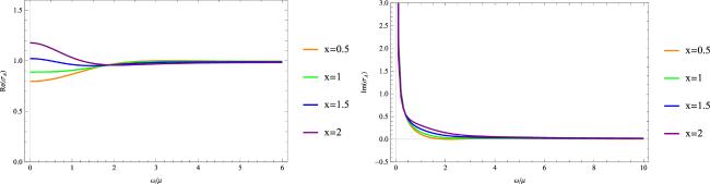
Figure 1. The real part (left) and the imaginary part (right) of the conductivity σA for various x = 0.5, 1, 1.5, 2 (orange, green, blue, purple) without momentum dissipation. The temperature is fixed at T/μ = 0.31. |
3.2.2. A case with momentum dissipation
Next, we consider the case where momentum dissipation is introduced, i.e. m ≠ 0. Although the translational symmetry has been broken due to the presence of the axions, our results show the conductivities σA, σB and γ in the normal phase still satisfy the symmetry (44 ), see appendix C for details.
We fix m/μ = 1 and compare the effect of increasing x on the conductivity σA in figure 2. Due to the presence of the momentum dissipation, the Drude peak is broadened and the DC conductivity becomes the finite value given by (17 ). We have checked that the DC limit of the numerics at ω = 0 agrees with the analytic value σA in (17 ).
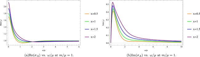
Figure 2. The real part of the conductivities σA (a) and the imaginary part of the conductivities σA (b) change with the different doping parameter x = 0.5, 1, 1.5, 2 (orange, green, blue, purple) at m/μ = 1. The temperature is fixed at T/μ = 0.31. |
We compare the conductivity γ with the different x in different cases in figure 3. Our results show that the values of the positive conductivities γ at ω = 0 increase with the increase of x in the case of m/μ = 1 in figure 3(b). On the contrary, the values of negative conductivities decrease accordingly without momentum dissipation in figure 3(a). This observation is very interesting, and we consider that it is the result of competition between the momentum dissipation that breaks the translational symmetry and the chemical potential.
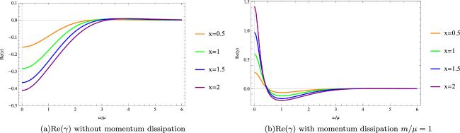
Figure 3. The conductivities γ change with the different doping parameter x = 0.5, 1, 1.5, 2 (orange, green, blue, purple) without momentum dissipation. (b) The conductivities γ change with the different doping parameter x = 0.5, 1, 1.5, 2 (orange, green, blue, purple) at m/μ = 1. The temperature is fixed at T/μ = 0.31. |
Figure 4 shows how the conductivity σA changes with different dissipation intensity m/μ at x = 2. Figure 4(a) is the real part and figure 4(b) is the imaginary part of the conductivity σA. We find that as m/μ increases, the value of $\mathrm{Re}({\sigma }_{A}$) at ω = 0 is smaller and the Drude peak disappears.
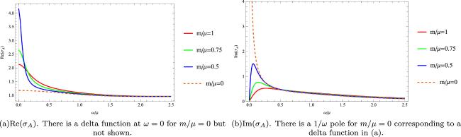
Figure 4. The real part of the conductivities σA (a) and the imaginary part of the conductivities σA (b) change with the different dissipation intensity m/μ = 1, 0.75, 0.5, 0 (red, green, blue, dashed) at T/μ = 0.31. |
We present the real part of the AC conductivities σA as functions of ω/μ for various Q/r0, in order to see the influence of the parameter Q related to the dilaton profile. We fix x = 2 and m/r0 = 0.5, here. As Q/r0 increases, the conductivity decreases at low frequencies and tends to a stable value at high frequencies. The AC conductivity is given by a constant value when Q = 0 corresponding the constant dilaton profile. A case Q = 0 corresponds to the constant dilaton profile, in which the AC conductivity is given by a constant value. The result in figure 5 agrees with the expected behavior. Note that T and μ functions of r0, Q, x and m, so they varies when we change Q. For fixed m and x, different Q/r0 corresponds to different T/μ.
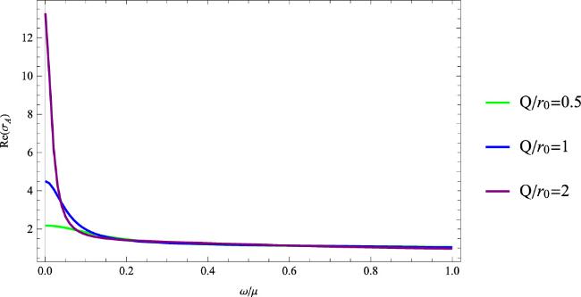
Figure 5. The real parts of conductivities σA change with ω/μ at different parameter Q/r0 = 0.5, 1, 2 (green, blue, purple) corresponding to T/μ = 0.445, 0.312, 0.219, respectively. We set m/r0 = 0.5. |
4. The superconducting dome
In this section, we investigate the phase diagram in x-T plane in our model. At the critical temperature, the spontaneous breaking of the U(1) symmetry is due to the condensation of scalar field χ in the bulk, and the superconducting instability corresponds to developing a non-trivial scalar χ. In order to investigate whether the boundary system exhibits a superconducting phase, we study the instability of the scalar hair around the normal phase of the dual bulk system. We solve the linearized equation of motion about χ in the background of (11 ) to determine the superconducting phase of the boundary system. Here, we assume that the phase transition is second order for simplicity, so we regard the onset of the charged scalar instability as a phase transition point.4(4 More precisely, we have to study the nonlinear condensation to see whether the phase transition is the second order. However, holographic models without a nonlinear potential term exhibit the second order phase transition usually. If the transition is a first order, the instability edge we investigate here does not agree with the phase transition points, but rather the edge of the metastable region of the normal phase.)
The phase transition is related to the formation of the scalar hair around the normal phase. When the temperature is below the critical temperature Tc, the system becomes unstable and the scalar hair begins to develop. In the vicinity of the temperature at which the system develops non-trivial scalar hair of χ, the value of χ should be small so we can consider it as a perturbation. Then, we solve the linear motion equation (2 ) of the scalar field χ in the normal phase background without taking backreaction into consideration. By making a coordinate transformation of the metric form (11 ) i.e., u = 1/r, (2 ) yields
$\begin{eqnarray}\begin{array}{l}\chi ^{\prime\prime} +\left(\displaystyle \frac{f^{\prime} }{f}+\displaystyle \frac{g^{\prime} }{g}-\displaystyle \frac{2}{u}\right)\chi ^{\prime} \\ \ +\ \displaystyle \frac{\chi \left(f\left({{au}}^{2}{A}_{t}{{\prime} }^{2}+{{bu}}^{2}{B}_{t}{{\prime} }^{2}+2{{cu}}^{2}{A}_{t}^{\prime} {B}_{t}^{\prime} -\tfrac{2{M}^{2}}{{u}^{2}}\right)+2n{\left({q}_{A}{A}_{t}+{q}_{B}{B}_{t}\right)}^{2}\right)}{2{f}^{2}}=0,\end{array}\end{eqnarray}$
where ‘prime’ stands for ∂u.To solve the equation (45 ), we need to impose appropriate boundary conditions. In the infrared (IR) limit, near the horizon, we impose the regular condition for the scalar field, this can be expressed as
$\begin{eqnarray}\chi (u)={\chi }_{h}^{(I)}+{\chi }_{h}^{({II})}(u-{u}_{h})+\displaystyle \frac{{\chi }_{h}^{({III})}}{2!}{\left(u-{u}_{h}\right)}^{2}+\cdots .\end{eqnarray}$
In the UV limit, near u = 0, χ has an asymptotic expansion of $\begin{eqnarray}\chi (u)={\chi }^{(-)}{u}^{3-{\rm{\Delta }}}+{\chi }^{(+)}{u}^{{\rm{\Delta }}}+\cdots ,\end{eqnarray}$
where Δ is a larger root of M2 = Δ(Δ − 3), and we fix the scaling dimension Δ = 5/2 following [21]. We also impose a condition to vanish the non-normalizable term. As a result, the solution of this two-point boundary values problem is a static zero mode which indicates onset of the instability.In the following, we fix the parameters (19 ) in the action. We also fix μ or ρA as a scale depending on whether considering in the grand canonical ensemble or the canonical ensemble, respectively. Here, we can also fix Q = 1 by virtue of the scaling symmetry without loss of generality. In other words, we can regard quantities scaled by Q, such as m/Q, uhQ, T/Q, μ/Q, as new quantities. Then, the leaving parameters are the translational symmetry breaking parameter m, the doping x and the location of the horizon uh. These are related to the temperature T and the chemical potential μ by (15 ) and (13 ), respectively. We look for the critical values (x, T) at which the boundary condition is satisfied for fixed m: the source coefficient χ(−) of the field χ near the boundary expansion disappears there. We can find the multiple sets of (x, T), but the outermost set in the x-T plane is expected to be dominant for the instability. We have also checked that the solution χ(u) for such a (x, T) has no node in its u-coordinate profile. In the following, we will only show the outermost set of (x, T) as a critical values.
Now, we test a set of model parameters with the following values:
$\begin{eqnarray}a=-10,\,b=-\displaystyle \frac{4}{3},\,c=14,\,n=1,\,{M}^{2}=-\displaystyle \frac{5}{4}.\end{eqnarray}$
Note that we have already fixed qA = 1 and qB = 0. Figure 6 shows the critical temperature Tc as a function of x for m = 0, by settings ρA as a scale, i.e., in the canonical ensemble.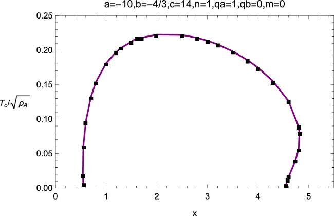
Figure 6. The critical temperature ${T}_{c}/\sqrt{{\rho }_{A}}$ versus the doping parameter x of the model ( |
In the grand canonical ensemble, we plot the critical temperature as a function of the doping parameter x by setting μ as a scale, as shown in figure 7. Here, we draw the phase diagram of the x-T plane with the translational symmetry breaking parameter m/μ = 0, 0.5. In both cases, we find that the dome shape does appear in the x-T plane. It can indeed be seen that the critical temperature Tc obtained by numerical calculation first increases and then decreases with the increase of doping, which is in line with the phase diagram characteristics of high temperature superconductors in reality. In the region near zero temperature, however, the phenomenon that the black dots near the endpoints shrink inward appears different from the previous model. As r0 → 0, i.e., uh → ∞ , the Gubser–Rocha model can reach zero temperature. The black dots near the two endpoints whose uh are large in our model, which fit the zero temperature conditions of the original Gubser–Rocha model [37]. Compared with former gravitational background researches, the Gubser–Rocha holographic high temperature-doped superconductor shows a difference in the region near zero temperature. We also prove that the introduction of translational symmetry breaking does not destroy the original superconducting dome structure in our extended model.
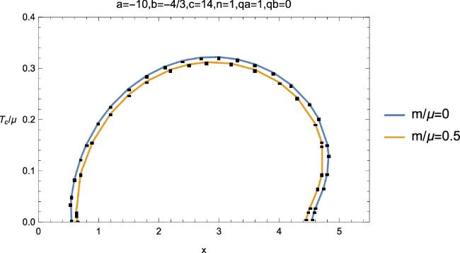
Figure 7. The phase diagram of the (x, Tc/μ) plane of the model ( |
We also discuss the influence of the value of coupling ‘c’ on the dome and obtain the same results as those obtained in [23]. We fix a = b = 0, m/μ = 0 and choose different c. The result is shown in figure 8. Our result indicates that the higher the value of c, the larger the dome. The action brought by the coupling of the two gauge fields is obviously the decisive factor leading to the emergence of the dome.
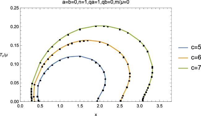
Figure 8. The phase diagram of the (x, Tc/μ) plane. We fix a =b = 0, m/μ = 0 and choose different c. The higher the value of c, the larger dome. |
With breaking translational symmetry, we reproduce the high-Tc superconducting dome in a black brane whose entropy is proportional to the near zero temperature. Similarly to figure 7, in the vicinity of absolute zero temperature, a clear trend emerges as the inward shrinking of the black dots near the endpoints. We also find that even if the coupling to a single gauge field is zero, relying on the cross term coupling, we can still obtain a superconducting dome. This is the main result of our paper.
5. Conclusion and discussion
In this paper, we studied the holographic theory of building a dome region in the temperature-doping plane like a realistic high-Tc superconductor. We attempt to realize a superconducting dome on the x − T plane phase diagram in the holographic superconductors model, namely the Gubser–Rocha model. We first calculate the DC conductivities in the normal phase analytically. Our results show the resistivity is proportional to temperature with the momentum dissipation in the normal phase. We then calculate conductivities associated to two gauge fields of our model in the normal phase numerically. We find there is a symmetry between σA, γ and σB with a specific doping parameter x in the normal phase. Our results indicate momentum dissipation cannot break this symmetry.
Furthermore, we investigated the phase diagram for the normal and superconducting phases. One of the main progresses of this paper is to show that the superconducting dome-shaped region exists in the extended Gubser–Rocha model in finite temperature with broken translational symmetry. This is a generalization of the previous work [23]. In comparison with other previous studies, the dome shrinks inward at both endpoints near zero temperature. This behavior might be caused by the presence of the dilaton field in our model. The parameter Q is closely related to the profile of the dilaton, while it is also involved in the temperature and chemical potential, and the number of parameters is the same as the Reissner–Nordström black hole case. Previous works show that the right boundary of the dome gently tends outward to zero temperature, and the experimental data is between our results and the previous studies. Our work provides a new possibility for a better simulation of the experimental phenomenon, which is worthy of further study. Moreover, our results show that larger coupling c makes the dome higher in this background, which also verified the role of the three point interaction −cχ2AμνBμν under the hyperscaling violation geometry.
In this study, we employed the holographic model based on the Gubser–Rocha model for the purpose of constructing the holographic model of strange metals with a doping parameter. As we have shown, the model can reproduce the typical behavior of the linear-T resistivity in some limits, not involving a magnetic field. However, the authors of [17] argued that the Gubser–Rocha model with linear axions cannot capture all of the strange metallic behaviors. We have to consider further improvements of the model to overcome the difficulties for reproducing the strange metallic behaviors by using the holography. In any case, doping should be introduced for constructing a realistic holographic superconducting model since it is a typical parameter in unconventional superconductors.
We have constructed a holographic s-wave doped superconductor closer to the realistic background in a Gubser–Rocha black brane whose entropy is proportional to near zero temperature. Since most unconventional superconductors have d-wave symmetry, we hope to extend the present work to d-wave holographic superconductors in the future. It would be interesting to follow the lines that we are studying here.
Acknowledgments
We would like to thank Xian-Hui Ge, Sang-Jin Sin, Blaise Goutéraux and Li Li for their valuable comments and discussions. This work is supported by the National Natural Science Foundation of China (Grant Nos. 12275166, 11875184, 12147158 and 11805117) and the NFSC-NFR joint program 12311540141.
Appendix A. The linearised equations in momentum space
In this section, we write the linearised equations of motion for the fluctuations studied in section 3 . These are obtained asA1 ), (A2 ), (A3 ) and (A4 ).
$\begin{eqnarray}\begin{array}{l}\displaystyle \frac{{\omega }^{2}{a}_{x}(r)}{f{\left(r\right)}^{2}}+\displaystyle \frac{{a}_{x}^{{\prime} }(r){f}^{{\prime} }(r)}{f(r)}+{a}_{x}^{{\prime} }(r){\varphi }^{{\prime} }(r)+\displaystyle \frac{{r}^{2}{h}_{{tx}}^{{\prime} }(r){A}_{t}^{{\prime} }(r)}{{r}_{0}^{2}f(r)}+{a}_{x}^{{\prime\prime} }(r)\\ +\ {h}_{{tx}}(r)\left(\displaystyle \frac{2{{rA}}_{t}^{{\prime} }(r)}{{r}_{0}^{2}f(r)}+\displaystyle \frac{{r}^{2}{\varphi }^{{\prime} }(r){A}_{t}^{{\prime} }(r)}{{r}_{0}^{2}f(r)}+\displaystyle \frac{{r}^{2}{A}_{t}^{{\prime\prime} }(r)}{{r}_{0}^{2}f(r)}\right)=0,\end{array}\end{eqnarray}$
$\begin{eqnarray}\begin{array}{l}\displaystyle \frac{{\omega }^{2}{b}_{x}(r)}{f{\left(r\right)}^{2}}+\displaystyle \frac{{b}_{x}^{{\prime} }(r){f}^{{\prime} }(r)}{f(r)}+{b}_{x}^{{\prime} }(r){\varphi }^{{\prime} }(r)+\displaystyle \frac{{r}^{2}{h}_{{tx}}^{{\prime} }(r){A}_{t}^{{\prime} }(r)}{{r}_{0}^{2}f(r)}+{b}_{x}^{{\prime\prime} }(r)\\ +\ {h}_{{tx}}(r)\left(\displaystyle \frac{2{{rB}}_{t}^{{\prime} }(r)}{{r}_{0}^{2}f(r)}+\displaystyle \frac{{r}^{2}{\varphi }^{{\prime} }(r){B}_{t}^{{\prime} }(r)}{{r}_{0}^{2}f(r)}+\displaystyle \frac{{r}^{2}{B}_{t}^{{\prime\prime} }(r)}{{r}_{0}^{2}f(r)}\right)=0,\end{array}\end{eqnarray}$
$\begin{eqnarray}\begin{array}{l}{{\rm{\Phi }}}_{x}^{{\prime\prime} }(r)+(\displaystyle \frac{f^{\prime} (r)}{f(r)}+\displaystyle \frac{g^{\prime} (r)}{g(r)}){{\rm{\Phi }}}_{x}^{{\prime} }(r)+\displaystyle \frac{{\omega }^{2}}{f{\left(r\right)}^{2}}{{\rm{\Phi }}}_{x}(r)-\ \displaystyle \frac{{{imr}}^{2}\omega {h}_{{tx}}(r)}{{r}_{0}^{2}f{\left(r\right)}^{2}g(r)}=0,\end{array}\end{eqnarray}$
$\begin{eqnarray}\begin{array}{l}\ {h}_{{tx}}(r)\left(\displaystyle \frac{2}{r}-\displaystyle \frac{{g}^{{\prime} }(r)}{g(r)}\right)+{h}_{{tx}}^{{\prime} }(r)+\displaystyle \frac{{{\rm{e}}}^{\varphi (r)}{r}_{0}^{2}}{{r}^{2}}\left({a}_{x}(r){A}_{t}^{{\prime} }(r)+{b}_{x}(r){B}_{t}^{{\prime} }(r)\right)+\ \displaystyle \frac{2{{imr}}_{0}^{2}f(r){{\rm{\Phi }}}_{x}^{{\prime} }(r)}{{r}^{2}\omega }=0,\end{array}\end{eqnarray}$
$\begin{eqnarray}\begin{array}{l}{h}_{{tx}}^{{\prime\prime} }(r)+\displaystyle \frac{4{h}_{{tx}}^{{\prime} }(r)}{r}+\displaystyle \frac{{{\rm{e}}}^{\varphi (r)}{r}_{0}^{2}}{{r}^{2}}({a}_{x}^{{\prime} }(r){A}_{t}^{{\prime} }(r)+{b}_{x}^{{\prime} }(r){B}_{t}^{{\prime} }(r))\\ -\ \displaystyle \frac{2{{\rm{i}}{mr}}_{0}^{2}\omega }{{r}^{2}f(r)}{{\rm{\Phi }}}_{x}(r)\\ +\ {h}_{{tx}}(r)\left(\displaystyle \frac{2}{{r}^{2}}+\displaystyle \frac{3}{f(r)}({{\rm{e}}}^{-\varphi (r)}+{{\rm{e}}}^{\varphi (r)})\right.\\ -\ \displaystyle \frac{{f}^{{\prime} }(r){g}^{{\prime} }(r)}{f(r)g(r)}+\displaystyle \frac{{g}^{{\prime} }{\left(r\right)}^{2}}{2g{\left(r\right)}^{2}}-\displaystyle \frac{3}{2}{\varphi }^{{\prime} }{\left(r\right)}^{2}\\ +\ \displaystyle \frac{{{\rm{e}}}^{\varphi (r)}}{2f(r)}({A}_{t}^{{\prime} }{\left(r\right)}^{2}+{B}_{t}^{{\prime} }{\left(r\right)}^{2})\\ \left.-\ \tfrac{{f}^{{\prime\prime} }(r)}{f(r)}-\tfrac{2{g}^{{\prime\prime} }(r)}{g(r)}-\tfrac{2{m}^{2}}{f(r)g(r)}\right)=0.\end{array}\end{eqnarray}$
The last equation can be obtained from the others. Thus, the set of independent equations are given by (Appendix B. Numerical details for the computation of the conductivities
In this section, we provide some details for the numerical computation of the electric/spin conductivities. The procedure is mostly the same as those explained in [50, 52]. However, we need to find suitable solutions depending on the methods for curing the problem of the degrees of freedom. Now, we write the bulk fluctuations as four components vectors $\delta {\rm{\Psi }}={({a}_{x},{b}_{x},{{\rm{\Phi }}}_{x},{h}_{{tx}})}^{T}$. Imposing the incoming-wave condition at the horizon, we obtain three independent solutions (δ$\Psi${1}, δ$\Psi${2} , δ$\Psi${3}) associated with the choice of the horizon values (${a}_{x}^{I}$ , ${b}_{x}^{I}$, ${{\rm{\Phi }}}_{x}^{I}$, ${h}_{{tx}}^{I}$) with the constraint. Note that the upper index in the braces denotes the label of the solution basis, here. We write these as the 3 × 4 matrix
$\begin{eqnarray}H(r):= (\delta {{\rm{\Psi }}}^{\{1\}}\quad \delta {{\rm{\Psi }}}^{\{2\}}\quad \delta {{\rm{\Psi }}}^{\{3\}}).\end{eqnarray}$
In the boundary constraint method, we also impose the constraint (40 ) on the boundary values. To find the linear combination satisfying the constraint, it is convenient to consider the following combination40 ) near the boundary. We define the 3 × 3 matrix as40 ) with ${\rm{m}}\,{\hat{h}}_{{tx}}^{(0)}\,=0.\delta {{\rm{\Psi }}}^{\{F\}}$ satisfies ${a}_{x}^{(0)}={b}_{x}^{(0)}=0$ and $m{\hat{h}}_{{tx}}^{(0)}=1$. For example, the electric conductivity σA is obtained by using $\delta {{\rm{\Psi }}}^{\{{a}_{x}\}}$.
$\begin{eqnarray}F(\omega ,r):= {{mh}}_{{tx}}(r)+{\rm{i}}\omega {r}_{0}^{2}{{\rm{\Phi }}}_{x}(r),\end{eqnarray}$
which gives the left-hand side of ( $\begin{eqnarray}\tilde{H}(r):= \left(\begin{array}{ccc}{a}_{x}^{\{1\}} & {a}_{x}^{\{2\}} & {a}_{x}^{\{3\}}\\ {b}_{x}^{\{1\}} & {b}_{x}^{\{2\}} & {b}_{x}^{\{3\}}\\ {F}^{\{1\}} & {F}^{\{2\}} & {F}^{\{3\}}\end{array}\right).\end{eqnarray}$
Using this matrix, we obtain the coefficients of the linear combination by ${\tilde{H}}^{-1}({r}_{b})$ with a large cutoff rb. We can construct the 3 × 4 solution matrix as $\begin{eqnarray}(\delta {{\rm{\Psi }}}^{\{{a}_{x}\}}\,\,\delta {{\rm{\Psi }}}^{\{{b}_{x}\}}\,\,\delta {{\rm{\Psi }}}^{\{F\}}):= H(r){\hat{H}}^{-1}({r}_{b}).\end{eqnarray}$
The solution $\delta {{\rm{\Psi }}}^{\{{a}_{x}\}}$ satisfies the Dirichlet conditions ${a}_{x}^{(0)}=1,{b}_{x}^{(0)}=0$ and the constraint (In the RGS method, we consider the extra solution (42 ) as one of the solution basis. Writing $\delta {{\rm{\Psi }}}^{\{4\}}\,={\left(0,0,m{\zeta }_{0},-{\rm{i}}\omega \displaystyle \frac{{r}_{0}^{2}}{{r}^{2}}g(r){\zeta }_{0}\right)}^{{\rm{T}}}$, we can make the 4 × 4 matrix
$\begin{eqnarray}{H}_{\mathrm{RGS}}(r):= (\delta {{\rm{\Psi }}}^{\{1\}}\quad \delta {{\rm{\Psi }}}^{\{2\}}\quad \delta {{\rm{\Psi }}}^{\{3\}}\quad \delta {{\rm{\Psi }}}^{\{4\}}),\end{eqnarray}$
where ζ0 is an arbitrary nonzero constant. Similar to the previous method, ${H}_{\mathrm{RGS}}^{-1}({r}_{b})$ gives the coefficients of the linear combination. Actually, taking the linear combination with δ$\Psi${4} implies considering the residual gauge transformation. We obtain the 4 × 4 solution matrix as $\begin{eqnarray}(\delta {{\rm{\Psi }}}_{\mathrm{RGS}}^{\{{a}_{x}\}}\quad \delta {{\rm{\Psi }}}_{\mathrm{RGS}}^{\{{b}_{x}\}}\quad \delta {{\rm{\Psi }}}_{\mathrm{RGS}}^{\{{{\rm{\Phi }}}_{x}\}}\quad \delta {{\rm{\Psi }}}_{\mathrm{RGS}}^{\{{h}_{{tx}}\}}):= {H}_{\mathrm{RGS}}(r){H}_{\mathrm{RGS}}^{-1}({r}_{b}).\end{eqnarray}$
Each solution simply satisfies the diagonal Dirichlet boundary conditions at the boundary. We can compute several conductivities by using these solutions. For example, the electric conductivity can be obtained by using $\delta {{\rm{\Psi }}}_{\mathrm{RGS}}^{\{{a}_{x}\}}$. As we have mentioned, the results of the conductivities are the same as those obtained in the first method.Appendix C. Symmetry between conductivities in normal phase
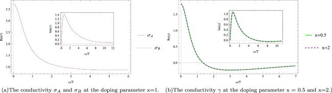
In this section, We present electrical conductivities in our model that support the conclusions that the conductivities σA, σB and γ satisfy the symmetry (44 ). In the case of no momentum dissipation, we show the real part of the conductivity σA and σB at x = 1 in figure 9(a), γ at x = 0.5 and x = 2 in figure 9(b), respectively. Figure 10 shows images of the conductivities with the momentum dissipation parameter m = 1. The fact that two lines coincide perfectly proves the symmetry of the system still exists after the translation symmetry is broken.
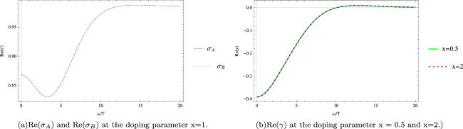
Figure 9. A case without momentum dissipation m = 0 at T = 0.33. (a) The real part of the conductivities σA and σB at x = 1. (b) The real part of the conductivity γ at x = 0.5 and x = 2. The two lines coincide perfectly. The system enjoys the symmetry. There is a delta function at ω = 0 but not shown. |
Figure 10. The conductivity σA and σB (a) and the conductivity γ (b) with momentum dissipation m = 1 at T = 0.33, the two lines coincide perfectly. The system still enjoys the symmetry. |