


1. Introduction
The current acceleration expansion of the Universe is one of the puzzles in modern cosmology. Reviewing general relativity and its field equations shows that the matter-radiation field, due to its gravitational effects, cannot explain current acceleration epoch. Keeping general relativity and its deep analyzing also reveals that the Universe may include another component with negative pressure [2]. The cosmological constant ${\rm{\Lambda }}$ as its simplest form can present such a field in large-scale structure with a constant equation of state ${\omega }_{{\rm{\Lambda }}}=-1$ [3]. However, this model suffers from two theoretical (fine-tuning) and cosmological (coincidence) problems [4]. In this context, a dozen different approaches are presented to alleviate these problems.
The modified theories of gravity are one of these straightforward scenarios. In such theories the usual Einstein–Hilbert action modified by different scalar terms built by the Riemann tensor and its derivatives [5–8], curvature-matter interaction terms [9–11] and or non-Einsteinian matter field [12, 13]. As result, dark energy given as extra terms in Friedmann equations depends on some linear and/or non-linear relation between geometry and matter. Although in most of these models, the modified theories of gravity support observations, there is no strong evidence around the validity of them, theoretically. For instance, according to the Rastall idea, one may assume that the conservation law is broken in curved spacetime and thus there is a flux of energy-momentum in non-flatness geometry due to the gravitational field [14]. This idea may open new windows to investigate field equations in high levels of gravity energy. However, this proposal in which the flux of the energy-momentum is proportional to the scalar curvature $R$ is questionable.
Studying relativistic thermodynamics in this case may give some robust clues in finding the flux of the energy-momentum tensor in special relativity, theoretically [15]. As discussed in [1], generalizing this model into curved spacetime yields a new modified theory of gravity that satisfies the main Rastall idea, ${{ \mathcal T }}_{\,\mu ;\nu }^{\nu }\ne 0,$ in which a flux of energy-momentum is given by the evolution of thermodynamical parameters and not the scalar curvature. Although such a theory of gravity alleviates the coincidence problem of the cosmological constant model, in the absence of a dark energy model when we face with the pure non-conserved theory of gravity, this alternative theory cannot explain the current acceleration phase. This issue traces back to its behavior in the Friedmann–Robertson–Walker Universe; one can assume extra terms in the time component of the field equation as density of dark energy, but there is no corresponding terms in the second Friedmann equation as pressure of dark energy. Unlike other alternative theories of gravity, it shows that the pure non-conserved theory gives no dark energy, directly. As a result, to investigate late-time Universe one needs to add the density of dark energy by hand. Hence, in this study, we will study one of the candidates of dark energy in a non-conserved theory of gravity, in which the density of the dark energy comes from the fundamental properties of quantum circumstance. Inspired by the investigation of the thermodynamics of a black hole [16], Hooft proposed the famous holographic principle [17]. According to this principle all of the information contained in a volume of space can be given as a hologram, which corresponds to a theory located on the boundary of that space. With this principle, Cohen and his collaborators suggested that in quantum field theory, a short distance cut-off is related to a long-distance cut-off due to the limit set by formations of a black hole [18]. With this idea at hand, the energy density of an unknown field is proportional to the square of the cut-off length, inversely i.e., ${\rho }_{0}\approx {{\ell }}^{-2}.$ A related idea was discussed in [19, 20], wherein ${\rho }_{0}$ given by the Hubble scale, ${\ell }={H}^{-1}.$ This selection alleviates the fine-tuning problem in which dark energy is scaled by the cosmological parameter and not the Planck length. However, this cut-off selection cannot explain the acceleration expansion of the Universe in late-time [21]. Consequently, it is worthwhile to explore such a model of dark energy in non-conserved theory and check whether this theory solves this problem or not.
The contents in this paper are organized as follows. In section 2, the non-conserved theory of gravity is revisited, briefly. In sections 3 and 4, late-time cosmology when the density of dark energy is given by ${\rho }_{X}\sim {H}^{2}$ is studied for non-interaction and interaction scenarios, respectively. We also explore viscous scenario in section 5. Remarks are given in section 6.
2. Covariant thermodynamics and new gravity models
The transformation of heat and temperature in relativity theory under the Lorentz group is one of the unsolved issues and opening topics in this theory. For instance, Einstein and Planck proposed [22, 23]
$\begin{eqnarray}\delta Q=\delta {Q}_{0}{\gamma }^{-1},T={T}_{0}{\gamma }^{-1},\end{eqnarray}$
while Ott and Arzelies proposed another transformation form [24, 25] $\begin{eqnarray}\delta Q=\delta {Q}_{0}\gamma ,T={T}_{0}\gamma .\end{eqnarray}$
where $\delta Q$ and $T$ denote heat and temperature, respectively, the variables with subscript $0$ represent those observed in the comoving frame, and $\gamma $ is the Lorentz factor. In addition to these options, Landsberg suggested that heat and temperature behave as absolute parameters and thus comoving and independent observers measure the same heat and temperature [26]. However, just two first options, (1) and (2), can satisfy a relativistic Carnot cycle [27]. The covariant form of relativity theory, in particular, may be essential to formulate relativistic laws of thermodynamics. In this context, one of the pioneer attempts are given by Israel and collaborators [15]: $\begin{eqnarray}\displaystyle \displaystyle \sum _{i}{S}_{\,i,\mu }^{\mu }=-\displaystyle \displaystyle \sum _{i}\left(\displaystyle \displaystyle \sum _{j}{\alpha }_{ji}\,{J}_{\,ji,\mu }^{\mu }+{\beta }_{\nu i}{{ \mathcal T }}_{i,\mu }^{\mu \nu }\right),\end{eqnarray}$
where the number of 4-vector ${J}_{ji}^{\mu }={n}_{ji}{u}^{\mu },$ represents the flux densities of conserved charges $j$ for component $i$-th and ${S}_{i}^{\mu }$ expresses the 4-flux of entropy of fluid $i$-th. ${\beta }_{\nu }={u}_{\nu }/{T}_{0}$ presents the inverse temperature 4-vector proposed by Van Kampen [28], and ${\alpha }_{j}={\zeta }_{j}/{T}_{0}.$ The parameter ${\zeta }_{j}$ denotes the relativistic injection energy or chemical potential per particle of type $j,$ related to its classical counterpart by: $\begin{eqnarray}{\zeta }_{j}={m}_{j}+{\zeta }_{j}^{\left({\rm{c}}{\rm{l}}{\rm{a}}{\rm{s}}{\rm{s}}{\rm{i}}{\rm{c}}\right)}.\end{eqnarray}$
It is to be noted that the 4-vector ${S}^{\mu }$ for the flux of entropy behaves in a similar way to the 4-vector for the flux of particle number. So, like the particle number that is the scalar for the comoving observer, it is shown that entropy in its comoving frame is a scalar as well [29]. As a result, this model is not in conflict with the standard expression of thermodynamical expression only when it is considered in a comoving frame. Relation (3) not only shows that Rastall’s idea is true in curved spacetime, but it is valid even in Minkowskian geometry when the flux of energy-momentum tensor is given as evolution in entropy and temperature of the whole system.To expand this model to curved geometry, one just needs to apply the principle of general relativity [1],6 ) actually proves Rastall’s idea, not only in the presence of the gravity but also for Minkowskian geometry. It should be noted that since the energy-momentum tensor in general relativity is a symmetric one, the right-hand side of equation (6 ) is also a symmetric tensor.
$\begin{eqnarray}\displaystyle \displaystyle \sum _{i}{S}_{\,i;\mu }^{\mu }=-\displaystyle \displaystyle \sum _{i}\left(\displaystyle \displaystyle \sum _{j}{\alpha }_{ji}{J}_{\,ji;\mu }^{\mu }+{\beta }_{\nu i}{{ \mathcal T }}_{i;\mu }^{\mu \nu }\right),\end{eqnarray}$
in which the usual (scalar) derivative is replaced by the covariant derivative. To derive and find the total energy-momentum tensor, one only needs to use definitions ${\beta }_{\nu }={u}_{\nu }/{T}_{0}$ and ${\alpha }_{j}={\zeta }_{j}/{T}_{0},$ which yields $\begin{eqnarray}\displaystyle \displaystyle \sum _{i}{{ \mathcal T }}_{i;\mu }^{\mu \nu }=\displaystyle \displaystyle \sum _{i}{u}_{i}^{\nu }\left({T}_{0}{S}_{\,i;\mu }^{\mu }+\displaystyle \displaystyle \sum _{j}{\zeta }_{ji}\,{J}_{\,ji;\mu }^{\mu }\right).\end{eqnarray}$
Such a relation shows that the flow of the energy-momentum tensor is a function of the thermodynamical parameters entropy, temperature, and mutual interaction among all participating particles. Equation (The general relativity principle is applied and after some manipulations, the field equations can be derived as such6 ) to (7 ). Defining the non-conserved term for each component participated in our system as7 ), namely
$\begin{eqnarray}{G}_{\mu \nu }-{\kappa }^{{\rm{{\prime} }}}\displaystyle \sum _{i}{u}_{\nu i}\left({T}_{0}{S}_{\mu i}+\displaystyle \sum _{j}{\zeta }_{{ji}}{J}_{j\mu i}\right)={\kappa }^{{\rm{{\prime} }}}\displaystyle \sum _{i}{{ \mathcal T }}_{\mu \nu i},\end{eqnarray}$
where $\kappa ^{\prime} $ is the proportional constant. Taking a covariant derivative of the above field equations and using ${G}_{\mu \nu ;\mu }=0$ recasts equations ( $\begin{eqnarray}{ {\mathcal E} }_{\mu \nu }={u}_{\nu }\left({T}_{0}{S}_{\mu }+\displaystyle \displaystyle \sum _{j}{\zeta }_{j}{J}_{j\mu }\right),\end{eqnarray}$
let one have compact form for field equation ( $\begin{eqnarray}{G}_{\mu \nu }-\kappa ^{\prime} \displaystyle \displaystyle \sum _{i}{ {\mathcal E} }_{\mu \nu i}=\kappa ^{\prime} \displaystyle \displaystyle \sum _{i}{{ \mathcal T }}_{\mu \nu i},\end{eqnarray}$
which shows each fluid (component) plays an explicit role in the field equations. Summation on all different components participating in the system (summation on index $i$), yields, $\begin{eqnarray}{G}_{\mu \nu }-{\kappa }^{{\rm{{\prime} }}}{{ \mathcal E }}_{\mu \nu }^{\left[e\right]}={\kappa }^{{\rm{{\prime} }}}{T}_{\mu \nu }^{\left[e\right]},\end{eqnarray}$
where we denote the effective terms ${ {\mathcal E} }_{\mu \nu }^{\left[e\right]}$ and ${T}_{\mu \nu }^{\left[e\right]}$ through $\begin{eqnarray}\displaystyle \sum _{i}{X}_{\mu \nu i}={X}_{\mu \nu }^{\left[e\right]},\end{eqnarray}$
when $X= {\mathcal E} $ and/or $T.$Since these field equations must shrink to standard Einstein field equations without losing generality, one can assume $\kappa ^{\prime} =\kappa .$
In the following we assume that the Universe is a homogenous and isotropic medium and describe with the Friedmann–Robertson–Walker metric10 ), the Friedmann equations become
$\begin{eqnarray}{\rm{d}}{s}^{2}=-{\rm{d}}{t}^{2}+{a}^{2}\left(\displaystyle \frac{{\rm{d}}{r}^{2}}{1-k{r}^{2}}+{r}^{2}{\rm{d}}{\theta }^{2}+{r}^{2}{\sin }^{2}\theta {\rm{d}}{\phi }^{2}\right),\end{eqnarray}$
where $a=a\left(t\right)$ is the cosmic scale factor and $k=0,$ $1$ and $-1$ corresponds to the flat, close, and open Universe, respectively. Observations confirm that the Universe is flat and thus we assume $k=0.$ With the aid of this assumption and using field equation ( $\begin{eqnarray}3{H}^{2}=\kappa \left({\rho }_{{\rm{m}}}+{ {\mathcal E} }_{tt}^{\left[e\right]}+{\rho }_{{\rm{X}}}\right),\end{eqnarray}$
$\begin{eqnarray}2\dot{H}+3{H}^{2}=-\kappa {p}_{{\rm{X}}},\end{eqnarray}$
in which we consider the matter as a dust field and subscripts $m$ and $X$ denote the matter and dark energy fields, respectively.With these Friedmann equations at hand, we will consider late-time Universe for non-interaction and interaction scenarios in the next two sections while dark energy density is given by the $\alpha $ as an arbitrary constant
$\begin{eqnarray}{\rho }_{{\rm{X}}}=\alpha {H}^{2}.\end{eqnarray}$
At the end of this section, we encourage interested readers to see the main paper of the non-conserved theory of gravity to review and check the effects of the cosmological constant and also the evolution of the Universe in the inflation era [1].3. Non-interaction scenarios
In this section, at first glance we will consider the Friedmann equations (13 ) and (14 ) for dark energy density given by equation (15 ) when there is no interaction between matter and dark energy. Plugging equation (15 ) into the first Friedmann equation (13 ) and solving it for the Hubble parameter yields,16 ) and density (15 ) directly reveals that the density of dark energy depends on the matter field and thus the coincidence problem alleviates. Moreover, if both density of matter and non-conserved term ${ {\mathcal E} }_{tt}^{\left[e\right]}$ can be positive, to have the valuable Hubble parameter, one finds out14 ), gives the continuity equation
$\begin{eqnarray}{H}^{2}=-\displaystyle \frac{\kappa }{\alpha \kappa -3}\left({\rho }_{{\rm{m}}}+{ {\mathcal E} }_{tt}^{\left[e\right]}\right),\end{eqnarray}$
Comparing the Hubble form ( $\begin{eqnarray}\alpha \kappa \lt 3.\end{eqnarray}$
Defining $x=\,\mathrm{ln}\left(a\right)$ and taking a derivative with respect to $x$ from the first Friedmann equation and using its result in equation ( $\begin{eqnarray}\begin{array}{c}{\rho }_{{\rm{m}}}^{{\prime} }+{ {\mathcal E} }_{tt}^{\left[e\right]^{\prime} }-\displaystyle \frac{\alpha \kappa }{\alpha \kappa -3}\left({\rho }_{{\rm{m}}}^{{\prime} }+{ {\mathcal E} }_{tt}^{\left[e\right]^{\prime} }\right)\\ +\,3\left[{\rho }_{{\rm{m}}}+{ {\mathcal E} }_{tt}^{\left[e\right]}-\displaystyle \frac{\alpha \kappa }{\alpha \kappa -3}\left({\rho }_{{\rm{m}}}+{ {\mathcal E} }_{tt}^{\left[e\right]}\right)+{p}_{{\rm{X}}}\right]=0,\end{array}\end{eqnarray}$
To reconstruct the standard density of matter, one may decouple the above equation as follows:
$\begin{eqnarray}{\rho }_{m}^{{\prime} }+3{\rho }_{m}=Q,\end{eqnarray}$
$\begin{eqnarray}\begin{array}{c}\displaystyle \frac{-\alpha \kappa }{\alpha \kappa -3}\left({\rho }_{{\rm{m}}}^{{\prime} }+\displaystyle \frac{3}{\alpha \kappa }{ {\mathcal E} }_{tt}^{\left[e\right]^{\prime} }\right)\\ +\,3\left[\displaystyle \frac{-\alpha \kappa }{\alpha \kappa -3}\left({\rho }_{{\rm{m}}}+\displaystyle \frac{3}{\alpha \kappa }{ {\mathcal E} }_{tt}^{\left[e\right]}\right)+{p}_{{\rm{X}}}\right]=-Q,\end{array}\end{eqnarray}$
where $Q$ represents the mutual interaction between the dark energy and matter field. With some computations and using the above equations, one finds:21 ) illustrates that the origin of the pressure of the dark energy is a non-conservation term in our model.
$\begin{eqnarray}{p}_{{\rm{X}}}=\displaystyle \frac{1}{\alpha \kappa -3}\left(3{ {\mathcal E} }_{tt}^{\left[e\right]}+{ {\mathcal E} }_{tt}^{\left[e\right]^{\prime} }+Q\right).\end{eqnarray}$
This expression of the pressure of the dark energy shows that in the non-interaction scenario, ${p}_{{\rm{X}}}$ is just the function of the non-conserved term ${ {\mathcal E} }_{tt}^{\left[e\right]}$ and its first derivative. As a result, equation (In the absence of enough microscopic observations of the interaction term, one may attempt to consider field equations (13 ) and (14 ) when $Q=0,$ (non-interaction scenario). However, since we are faced with an extra parameter ${ {\mathcal E} }_{tt}^{\left[e\right]}$ in our model, in this step it is necessary to have a valuable form for that. Reconsidering equation (8 ) reveals that it includes two parts: ${T}_{0}{S}_{t}$ and all interactions among particles. Keeping to the second law of thermodynamics shows that ${T}_{0}{S}_{t}$ must grow up with time, and thus it can be given by ${e}^{\gamma x}$ in which $\gamma \gt 0,$ while due to relation (4), the second part is proportional to the density of the matter field, namely
$\begin{eqnarray}\displaystyle \displaystyle \sum _{j}{\zeta }_{j}{J}_{jt}\propto {\rho }_{{\rm{m}}}.\end{eqnarray}$
Consequently with these assumptions for the expanding Universe, we may suggest that $\begin{eqnarray}{ {\mathcal E} }_{tt}^{\left[e\right]}=\beta {e}^{\gamma x}+\eta {\rho }_{{\rm{m}}},\end{eqnarray}$
where $\beta $ and $\eta $ are proportional constants.As a result and in the absence of the interaction term, $Q=0,$ the density of the matter, and the density and pressure of the dark energy are,
$\begin{eqnarray}{\rho }_{{\rm{m}}}={\rho }_{{\rm{m}}0}{{\rm{e}}}^{-3x},\end{eqnarray}$
$\begin{eqnarray}{\rho }_{{\rm{X}}}=-\displaystyle \frac{\alpha \kappa }{\alpha \kappa -1}\left(\left(1+\eta \right){\rho }_{{\rm{m}}0}{{\rm{e}}}^{-3x}+\beta {{\rm{e}}}^{\gamma x}\right),\end{eqnarray}$
$\begin{eqnarray}{p}_{{\rm{X}}}=\displaystyle \frac{\beta \left(3+\gamma \right)}{\alpha \kappa -1}{{\rm{e}}}^{\gamma x}\end{eqnarray}$
respectively.For such a dark energy model, the equation of the state and deceleration parameter given by:16 ) and (27 ), two free parameters $\beta $ and $\eta $ become28 ) obtains $\alpha $ as a function of ${x}_{T}$ when $q\left({x}_{T}\right)=0$ is used
$\begin{eqnarray}\begin{array}{c}{\omega }_{{\rm{X}}}=\displaystyle \frac{{p}_{{\rm{X}}}}{{\rho }_{{\rm{X}}}}=-1\\ \,+\,\displaystyle \frac{\alpha \kappa {\rho }_{{\rm{m}}0}\left(1+\eta \right){{\rm{e}}}^{-3x}-\beta \left(3+\gamma -\alpha \kappa \right){{\rm{e}}}^{\gamma x}}{\alpha \kappa \left({\rho }_{{\rm{m}}0}{{\rm{e}}}^{-3x}+\beta {{\rm{e}}}^{\gamma x}\right)},\end{array}\end{eqnarray}$
$\begin{eqnarray}q=\displaystyle \frac{1}{2}\left(1-\displaystyle \frac{\beta \left(3+\gamma \right){{\rm{e}}}^{\gamma x}}{{\rho }_{{\rm{m}}0}\left(1+\eta \right){{\rm{e}}}^{-3x}+\beta {{\rm{e}}}^{\gamma x}}\right).\end{eqnarray}$
To constrain the model with current observations, we set ${H}_{0}=67.4,$ ${{\rm{\Omega }}}_{m0}=0.315$ and ${\omega }_{X0}=-1$ [30], wherein ${{\rm{\Omega }}}_{{\rm{m}}0}$ is a current fractional density of the dust matter, defined by $\begin{eqnarray}{{\rm{\Omega }}}_{{\rm{m}}0}=\displaystyle \frac{\kappa {\rho }_{{\rm{m}}0}}{3{H}_{0}^{2}}.\end{eqnarray}$
Hence, and by using equations ( $\begin{eqnarray}\beta =\displaystyle \frac{\alpha \left(3-\alpha \kappa \right){H}_{0}^{2}}{3+\gamma },\end{eqnarray}$
$\begin{eqnarray}\eta =-1+\displaystyle \frac{1}{{{\rm{\Omega }}}_{{\rm{m}}0}}-\displaystyle \frac{\alpha \kappa \left(6+\gamma -\alpha \kappa \right)}{3{{\rm{\Omega }}}_{{\rm{m}}0}\left(3+\gamma \right)}.\end{eqnarray}$
In order to constrain $\alpha ,$ one may use the approach given in [31, 32]. In such an approach, defining the transition redshift $\begin{eqnarray}{x}_{T}=\,\mathrm{ln}\left(\displaystyle \frac{1}{1+{z}_{T}}\right),\end{eqnarray}$
with the aid of the deceleration parameter ( $\begin{eqnarray}\alpha =\displaystyle \frac{\left(3+\gamma \right){{\rm{e}}}^{-3{x}_{T}}}{\kappa \left(\left(2+\gamma \right){{\rm{e}}}^{\gamma {x}_{T}}+{{\rm{e}}}^{-3{x}_{T}}\right)}.\end{eqnarray}$
The joint analysis of SNe+CMB data and the ${\rm{\Lambda }}$ cold dark matter (CDM) theory obtains ${z}_{T}=0.52-0.73$ [33]. With this range at hand, the free parameter $\alpha $ is given by these observations.
In figures 1 and 2 the evolution of the equation of the state and the deceleration parameter as a function of the redshift $z$ for $\gamma =0.1$ and $1.1$ are plotted1(1 With these values of $\gamma ,$ the condition (14) is satisfied.). As shown, our model is valuable due to the non-conservation effects presented, while in the absence of the non-conservation term, the holographic dark energy ${\rho }_{X}=\alpha {H}^{2}$ evolves like pressureless matter during the expansion of the Universe, ${\omega }_{X}=0$ [21], and thus it cannot explain the current epoch. As plotted in figure 1, the dark energy in this model behaves like a dust matter field in the past Universe, coinciding with ${\rm{\Lambda }}$ CDM theory at $z=0$ and evolving like a phantom fluid in the future. From figure 2, since $q\to 0.5$ for $z\gg 0,$ there are no deviations in matter structure formation during the matter-dominated era. Furthermore, restricting $\alpha $ with a transition point shows that the model is not in conflict with the observations [33].
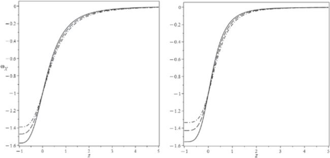
Figure 1. The equation of the state of the dark energy in the non-interaction scenario when ${H}_{0}=67.4$ and ${{\rm{\Omega }}}_{{\rm{m}}0}=0.315$ and $\gamma =0.1$ (left panel) and $\gamma =1.1$ (right panel) for ${z}_{T}=0.52$ (solid curve), ${z}_{T}=0.62$ (dashed curve) and ${z}_{T}=0.72$ (dash-dotted curve). |
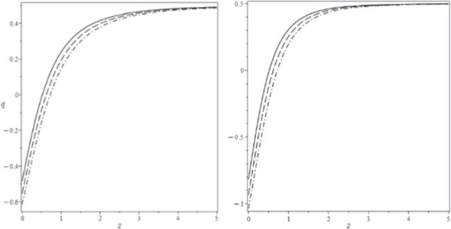
Figure 2. Deceleration parameter in the non-interaction scenario when $\gamma =0.1$ (left panel) and $\gamma =1.1$ (right panel) for ${z}_{T}=0.52$ (solid curve), ${z}_{T}=0.62$ (dashed curve) and ${z}_{T}=0.72$ (dash-dotted curve). |
To explore the effects of the perturbations on the classical stability of the model, the speed of sound squared ${\nu }_{c}^{2}$ should be positive and $\leqslant 1.$ 30 ) and (31 ), one obtains
$\begin{eqnarray}{\nu }_{c}^{2}=\displaystyle \frac{{\rm{d}}{p}_{{\rm{X}}}}{{\rm{d}}{\rho }_{{\rm{X}}}}=\displaystyle \frac{\partial {p}_{{\rm{X}}}}{\partial x}{\left(\displaystyle \frac{\partial {\rho }_{{\rm{X}}}}{\partial x}\right)}^{-1},\end{eqnarray}$
With the aid of equations ( $\begin{eqnarray}{\nu }_{c}^{2}=-\displaystyle \frac{\beta \gamma \left(3+\gamma \right){{\rm{e}}}^{\gamma x}}{\alpha \kappa \left(\beta \gamma {{\rm{e}}}^{\gamma x}-3{\rho }_{{\rm{m}}0}\left(1+\eta \right){{\rm{e}}}^{-3x}\right)},\end{eqnarray}$
The speed of sound squared ${\nu }_{c}^{2}$ as a function of the redshift for $\gamma =0.1$ and $1.1$ is plotted in figure 3. As shown, for $\gamma \gt 1,$ the model is instable classically for some values of transition points and thus we should have $0\lt \gamma \leqslant 1.$
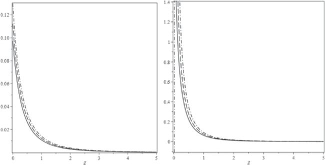
Figure 3. The speed of sound squared versus the redshift for the non-interaction scenario when $\gamma =0.1$ (left panel) and $\gamma =1.1$ (right panel) for ${z}_{T}=0.52$ (solid curve), ${z}_{T}=0.62$ (dashed curve) and ${z}_{T}=0.72$ (dash-dotted curve). |
As discussed in this section, it is revealed that the non-conservation term alleviates the original holographic model of the dark energy problem in which it can onset a trigger of current acceleration expansion.
In the two next sections, we will explore the interaction and pure viscous scenarios for our model.
4. Interaction scenarios
In this section, we assume that the interaction term $Q\ne 0$, given by $Q={c}_{1}\left({\rho }_{m}+{ {\mathcal E} }_{tt}^{\left[e\right]}\right)$ in which ${c}_{1}$, is an arbitrary constant. With this assumption, and using equations (16 ) and (19 ), the density of the matter field and dark energy is given by
$\begin{eqnarray}{\rho }_{{\rm{m}}}={c}_{2}{{\rm{e}}}^{\left({c}_{1}\left(1+\eta \right)-3\right)x}+\displaystyle \frac{\beta {c}_{1}}{3+\gamma -{c}_{1}\left(1+\eta \right)}{{\rm{e}}}^{\gamma x},\end{eqnarray}$
$\begin{eqnarray}\begin{array}{c}{\rho }_{{\rm{X}}}=-\displaystyle \frac{\alpha \kappa {c}_{2}\left(1+\eta \right)}{\alpha \kappa -3}{{\rm{e}}}^{\left({c}_{1}\left(1+\eta \right)-3\right)x}\\ \,-\,\displaystyle \frac{\alpha \beta \kappa {\left(3+\gamma \right)}^{2}}{\left(\alpha \kappa -3\right)\left(3+\gamma -{c}_{1}\left(1+\gamma \right)\right)}{{\rm{e}}}^{\gamma x}.\end{array}\end{eqnarray}$
As a result, the pressure for the corresponding dark energy becomes $\begin{eqnarray}\begin{array}{c}{p}_{{\rm{X}}}=\displaystyle \frac{{c}_{1}{c}_{2}{\left(1+\eta \right)}^{2}}{\alpha \kappa -3}{{\rm{e}}}^{\left({c}_{1}\left(1+\eta \right)-3\right)x}\\ \,+\,\displaystyle \frac{\beta {\left(3+\gamma \right)}^{2}}{\left(\alpha \kappa -3\right)\left(3+\gamma -{c}_{1}\left(1+\gamma \right)\right)}{{\rm{e}}}^{\gamma x}.\end{array}\end{eqnarray}$
Consequently, with the same initial conditions constraining model with the current values of the Hubble parameter and the fractional density of matter, one has $\begin{eqnarray}\beta =-\displaystyle \frac{\left(\alpha \kappa -3\right){H}_{0}^{2}}{\kappa }\left[\displaystyle \frac{\alpha \kappa \left({c}_{1}{H}_{0}^{2}+\kappa {\rho }_{{\rm{m}}0}\right)-3{c}_{1}{H}_{0}^{2}}{\kappa \left(\alpha {c}_{1}{H}_{0}^{2}+\left(3+\gamma \right)\,{\rho }_{{\rm{m}}0}\right)-3{c}_{1}{H}_{0}^{2}}\right],\end{eqnarray}$
$\begin{eqnarray}\eta =-\displaystyle \frac{\left(\alpha \kappa -3\right)\left(3+\gamma +{c}_{1}-\alpha \kappa \right){H}_{0}^{2}+\left(3+\gamma \right)\kappa {\rho }_{{\rm{m}}0}}{{c}_{1}\left(\alpha \kappa -3\right){H}_{0}^{2}+\left(3+\gamma \right)\kappa {\rho }_{{\rm{m}}0}},\end{eqnarray}$
$\begin{eqnarray}{c}_{2}=\displaystyle \frac{{\left(-3{c}_{1}{H}_{0}^{2}+\left(\alpha {c}_{1}{H}_{0}^{2}+\left(3+\gamma \right){\rho }_{{\rm{m}}0}\right)\right)}^{2}}{\kappa {c}_{1}\left(\alpha \kappa -3\right)\left(3+2\gamma -\alpha \kappa \right){H}_{0}^{2}+{\kappa }^{2}{\left(3+\gamma \right)}^{2}{\rho }_{{\rm{m}}0}}.\end{eqnarray}$
The volution of the equation of state, deceleration parameter, and speed of sound squared for this scenario is plotted in figures 4–6, which depicts that the model is not in conflict with the ${\rm{\Lambda }}$ CDM theory. As shown in figure 3, this model presents quintessence dark energy fluid and behaves like dust matter in high redshift while coinciding with the ${\rm{\Lambda }}$ theory at $z=0.$ Investigating the deceleration parameter just shows that the transition point in the interaction scenario satisfies the observations (see figure 4).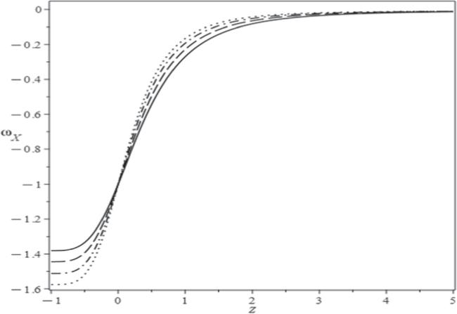
Figure 4. Equation of state for the interaction scenario when ${H}_{0}=67.4,$ ${{\rm{\Omega }}}_{{\rm{m}}0}=0.315$ and ${c}_{1}=\alpha =0.1$ is used for $\gamma =0.47$ (solid curve), $\gamma =0.63$ (dashed curve), $\gamma =0.8$ (dash-dotted curve) and $\gamma =0.96$ for dotted curve. |
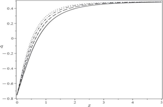
Figure 5. The deceleration parameter versus the redshift when ${H}_{0}=67.4,$ ${{\rm{\Omega }}}_{{\rm{m}}0}=0.315$ and ${c}_{1}=\alpha =0.1$ is used for $\gamma =0.47$ (solid curve), $\gamma =0.63$ (dashed curve), $\gamma =0.8$ (dash-dotted curve) and $\gamma =0.96$ for dotted curve. |
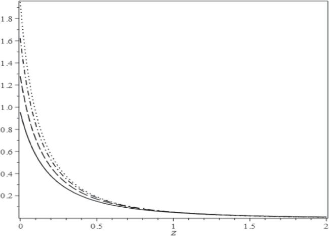
Figure 6. Speed of sound squared as the function of the redshift $z$ for $\gamma =0.47$ (solid curve), $\gamma =0.63$ (dashed curve), $\gamma =0.8$ (dash-dotted curve) and $\gamma =0.96$ for dotted curve when ${H}_{0}=67.4,$ ${{\rm{\Omega }}}_{{\rm{m}}0}=0.315$ and ${c}_{1}=\alpha =0.1.$. |
5. Viscous model
In this section, we study the bulk viscosity on holographic dark energy in the non-conserved theory of gravity. The bulk viscosity scenario is introduced by dissipating just through redefining the effective pressure ${p}^{\left[e\right]}=p-\zeta H$ where $\zeta $ is the bulk viscosity coefficient.
In the absence of interaction between the dust matter field and the dark energy, using equation (18 ) yields the effective pressure of viscous dark energy as15 ). In the following and as a toy model, we assume that $\zeta =\sigma {\rho }_{X}^{\tau }.$ Hence, with aid of equation (15 ), the bulk viscosity term is given by
$\begin{eqnarray}{p}_{{\rm{X}}}=\displaystyle \frac{1}{\alpha \kappa -3}\left(3{ {\mathcal E} }_{tt}^{\left[e\right]}+{ {\mathcal E} }_{tt}^{\left[e\right]^{\prime} }\right)+\zeta H.\end{eqnarray}$
Here, we are interested in exploring the Universe dominated by a dust matter field and the holographic dark energy given in equation ( $\begin{eqnarray}\zeta H=\sigma {\alpha }^{\tau }{H}^{1+2\tau }.\end{eqnarray}$
Computing the equation of state, deceleration parameter and speed of sound squared, one finds32 ) for deceleration parameter (46 ) obtains44 )–(46 ) are plotted when we set $\beta =110$ and $\gamma =0.1.$ As shown, the viscous dark energy gives another way to alleviate the transition point while the dark energy evolves as matter fluid in the past Universe to a cosmological constant-like model in $z=0$ and behaves like a strong phantom field in the future.
$\begin{eqnarray}{\omega }_{X}=1+\displaystyle \frac{\sigma }{\kappa \sqrt{\alpha }}{{\rm{\Upsilon }}}^{\tau -1/2}-\displaystyle \frac{\beta \left(3+\gamma \right){{\rm{e}}}^{\gamma x}}{\alpha \kappa \chi },\end{eqnarray}$
$\begin{eqnarray}q=\displaystyle \frac{1}{2}\left(1+\sigma \sqrt{\alpha }{{\rm{\Upsilon }}}^{\tau -1/2}-\displaystyle \frac{\beta \left(3+\gamma \right){{\rm{e}}}^{\gamma x}}{2\chi }\right),\end{eqnarray}$
$\begin{eqnarray}{\nu }_{c}^{2}=\displaystyle \frac{3\sigma }{\kappa \sqrt{\alpha }}\left(\tau +\displaystyle \frac{1}{2}\right){{\rm{\Upsilon }}}^{\tau -1/2}-\displaystyle \frac{\beta \gamma \left(3+\gamma \right){{\rm{e}}}^{\gamma x}}{\alpha \kappa {\chi }^{{\rm{{\prime} }}}},\end{eqnarray}$
in which the prime denotes the derivative with respect to $x$ and we define $\begin{eqnarray}\chi ={\rho }_{m0}\left(1+\eta \right){{\rm{e}}}^{-3x}+\beta {{\rm{e}}}^{\gamma x},\end{eqnarray}$
$\begin{eqnarray}{\rm{\Upsilon }}=-\displaystyle \frac{\alpha \kappa \chi }{\alpha \kappa -3}.\end{eqnarray}$
Constraining the model for the current Universe, $x=0,$ when ${\omega }_{{\rm{X}}0}=-1,$ we have $\begin{eqnarray}\alpha =\displaystyle \frac{3}{\kappa }-\displaystyle \frac{\beta +\left(1+\eta \right){\rho }_{{\rm{m}}0}}{{H}_{0}^{2}},\end{eqnarray}$
$\begin{eqnarray}\begin{array}{c}\sigma =\left(\displaystyle \frac{2\left(\left(1+\eta \right){\rho }_{{\rm{m}}0}+\beta \right)}{{H}_{0}}\right.\\ \,\left.-\,\displaystyle \frac{{H}_{0}\left(6\left(1+\eta \right){\rho }_{{\rm{m}}0}+\beta \left(3-\gamma \right)\right)}{\kappa \left(\left(1+\eta \right){\rho }_{{\rm{m}}0}+\beta \right)}\right){\left({H}_{0}^{2}\alpha \right)}^{-\tau }.\end{array}\end{eqnarray}$
Using transition point ( $\begin{eqnarray}\begin{array}{c}\tau =1+\tfrac{\mathrm{ln}\left({H}_{0}^{2}\right)}{2}\\ -\,\displaystyle \frac{\mathrm{ln}\left(\tfrac{6\chi \left(0\right)-\beta \left(3+\gamma \right)}{{H}_{0}\left(\chi \left({x}_{T}\right)-\beta \left(3+\gamma \right){{\rm{e}}}^{\gamma \chi \left({x}_{T}\right)}\right)}-\tfrac{2\kappa {\left(\left(1+\eta \right){\rho }_{m0}+\beta \right)}^{2}}{{H}_{0}^{3}\left(\chi \left({x}_{T}\right)-\beta \left(3+\gamma \right){{\rm{e}}}^{\gamma \chi \left({x}_{T}\right)}\right)}\right)}{\mathrm{ln}\left(\tfrac{\chi \left({x}_{T}\right)}{\chi \left(0\right)}\right)}.\end{array}\end{eqnarray}$
In figures 7–9, the evolution of the parameters given in equations (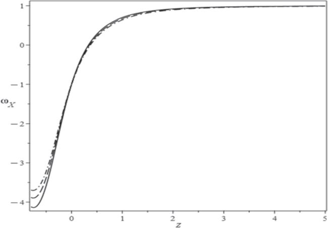
Figure 7. Equation of the state versus the redshift for ${z}_{T}=0.52$ (solid curve), ${z}_{T}=0.55$ (dashed curve) and ${z}_{T}=0.58$ (dash-dotted curve). |
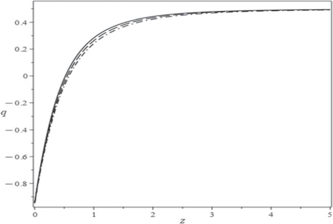
Figure 8. The evolution of the deceleration parameter as a function of the redshift for ${z}_{T}=0.52$ (solid curve), ${z}_{T}=0.55$ (dashed curve) and ${z}_{T}=0.58$ (dash-dotted curve). |

Figure 9. The speed of sound squared ${v}_{c}^{2}$ for the viscous model when we use ${z}_{T}=0.52$ (solid curve), ${z}_{T}=0.55$ (dashed curve) and ${z}_{T}=0.58$ (dash-dotted curve). |
6. Conclusions
To summarize, we have considered the original holographic dark energy in a new modified theory of gravity, ‘non-conserved gravity’. As discussed, in this theory the Rastall idea is reconsidered and shows that the energy-momentum tensor is not conserved when its flux is given by thermodynamical parameters of the system. Also, such a theory cannot present a current acceleration phase alone, and thus one needs to dilute the theory with other modified theories of gravity or add some parameters of dark energy by hand.
In this study, we have attempted to check the original holographic dark energy in which a cut-off length is proportional to the inverse of the Hubble parameter, i.e., ${\ell }={H}^{-1}.$ This model of dark energy cannot onset a late-time acceleration epoch in standard gravity theory as shown, due to the effects of the non-conservation term in our model, such a scenario of dark energy can explain the present phase. As discussed, in both non-interaction and interaction scenarios, the model presents dark energy which behaves like the cosmological constant at $z=0$, while for high redshifts it evolves as dust matter. However, such quintessence dark energy behaves as a phantom field in the future Universe. Futhremore, this dark energy is stable, wherein for both scenarios one finds ${v}_{c}^{2}\geqslant 0.$
As another plausible scenario we have studied the viscous model. As shown, this scenario also satisfies our observations. In this scenario, the dark energy, due to its viscosity, presents matter with positive pressure in the past Universe while in the current Universe, it coincides with the ${\rm{\Lambda }}$ CDM model.
We encourage any interested researchers to apply another dark energy model in the non-conserved theory of gravity to investigate and check this theory theoretically and observationally.