


1. Introduction
The relationship between mechanical force and the structural transitions of biomolecules has always been a focus in biophysical and mechanobiology researches. Over the years, single-molecule manipulation experiments have emerged as an important technique to measure the mechanical stability and force response of biomolecules [1–9]. In single-molecule manipulation experiments, the force-dependent conformation transition rates of biomolecules are the most important data to be measured [10]. The force range is always desired to be as wide as possible since it is important to reveal the detailed information of the underlying free-energy landscape, which determines the dynamic properties of biomolecules [11].
Constant loading rates and constant pulling speeds are usually applied in magnetic tweezers (MT) and atomic force microscopy (AFM)/optical tweezers (OT) experiments, respectively [1–9]. These measurements have provided kinetic parameters of various molecular systems [3–6]. In the case of constant loading rate in MT experiments, the unfolding force of proteins can be derived as an analytical equation for biomolecules following Bell’s model. The equation can be used to fit the experimental data to obtain kinetic parameters such as unfolding distance and zero-force unfolding rate [12, 13]. On the other hand, constant pulling speed experiments using AFM and OT can generate an average loading rate within a certain range. Although not very strict, the same analysis method can be used to obtain the kinetic properties [1].
However, a significant limitation with the constant loading rate method is that the extracted force-dependent transition rates are confined to limited force range with non-zero force distribution. To obtain transition rates over a large force range, different loading rates with orders of magnitude difference usually need to be applied [14]. Force is approximately an exponential function of the distance between permanent magnets and the sample in MT [figure 1]. Therefore, the magnets need to move nonlinearly to obtain a constant loading rate with an initial fast speed, which makes the mechanical control complex and limits the range of loading rate feasible in MT [15].
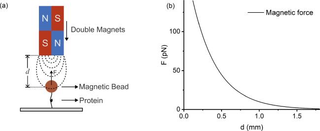
Figure 1. Schematic diagram of magnetic tweezers setup. (a) The force exerted on a protein molecule by a magnetic bead within the magnetic field of the double magnets. (b) The relationship between the force F and the distance d between the magnets and the paramagnetic bead is assumed to be $F(d)=200\exp (-3d)$ pN, where d is in units of millimeters. |
Another experimental strategy is to measure the waiting time of transitions at a series of constant forces. At forces with slow transitions, the stability of the equipment is crucial for the measurement. MT has the advantage of stability for long-time measurements over AFM and OT [3, 7]. On the other hand, if the transition is very fast, the process of the force jumping will give a dead time of measurement, which limits the fastest measurable transition rate [16].
In this study, we venture beyond the traditional realm of constant loading rate or constant force measurements and study the consequence of nonlinear force-loading controls. First, we derived the unfolding force distribution under exponential or exponential squared force-loading functions for Bell’s model. Second, a theoretical force versus time function was derived to render a uniform unfolding force distribution. By integrating traditional methods with innovative nonlinear force control, accurate unfolding rates can be achieved over a broader force range to enhance the efficiency of single-molecule manipulation experiments.
2. Model and methods
2.1. Force-dependent unfolding rate ku(F)
We conventionally conceptualize the unfolding of a protein as a process of overcoming a free-energy barrier [17, 18]. As the barrier height is affected by the stretching force, the unfolding rate ku is dependent on stretching force F. In this study, we suppose that the unfolding transition of a protein follows Bell’s model, whose force-dependent unfolding rate is given by [12],
$\begin{eqnarray}{k}_{{\rm{u}}}(F)={k}_{0}\exp (\beta {x}_{{\rm{u}}}F),\end{eqnarray}$
where k0 denotes the zero-force unfolding rate, xu the unfolding distance, i.e. the distance between the native state and transition state, β = 1/kBT, kB the Boltzmann constant and T the absolute temperature. In this study, unless otherwise specified, we set parameters k0 = 0.005 s−1 and xu = 2 nm.2.2. Force-loading function F(t)
The force-loading function, F(t), defines the force F as a function of time t. The linear force-loading function:
$\begin{eqnarray}F(t)={F}_{0}+{rt},\end{eqnarray}$
where F0 denotes the initial force and r the loading rate. Two kinds of nonlinear force-loading functions under scrutiny are the exponential function: $\begin{eqnarray}F(t)={F}_{0}\exp ({v}_{0}t),\end{eqnarray}$
and the exponential squared function: $\begin{eqnarray}F(t)={F}_{0}\exp ({a}_{0}{t}^{2}),\end{eqnarray}$
where v0 and a0 are parameters determining how fast the force increases.The double exponential function has been used to fit the force as a function of distance d between the magnets and the sample [15]. In this study, for simplicity, we suppose that the force in magnetic tweezers is an exponential function $F(d)=200\exp (-3d)$ pN, with d in units of millimeters [figure 1].
2.3. Simulation to obtain unfolding force distribution P(F)
Given the known force-dependent unfolding rate ku(F) of a protein and the force-loading function F(t), the unfolding process can be simulated using a Monte Carlo simulator [19]. The initial state of the protein is its native state N. The entire simulation process is coarse-grained into a random event chain with a time interval of Δt per frame. The probability of the protein unfolding in each frame is ku(F)Δt. When the protein molecule unfolds, the simulation stops, and the unfolding force is recorded. The unfolding force distribution P(F) can be obtained by the statistical histogram of unfolding forces from multiple repeated simulations.
2.4. Relationship between F(t), ku(F) and P(F)
From the known ku(F) and F(t), P(F) can also be derived analytically or numerically. Since the initial state is native state N, the survival probability of N state S(t) obeys the differential equation:
$\begin{eqnarray*}\displaystyle \frac{{\rm{d}}S(t)}{{\rm{d}}t}=-{k}_{{\rm{u}}}(F(t))S(t).\end{eqnarray*}$
with initial condition S(0) = 1, and $\begin{eqnarray*}P(F)=\displaystyle \frac{-{\rm{d}}S(t)/{\rm{d}}t}{{\rm{d}}F(t)/{\rm{d}}t}.\end{eqnarray*}$
Therefore, P(F) is given by equation: $\begin{eqnarray}P(F)=\displaystyle \frac{{k}_{{\rm{u}}}(F)}{\dot{F}(F)}\exp \left(-{\int }_{{F}_{0}}^{F}{k}_{{\rm{u}}}(f)/\dot{F}(f){\rm{d}}f\right),\end{eqnarray}$
where $\dot{F}={\rm{d}}F/{\rm{d}}t$ [20–22].In single-molecule manipulation experiments, we control F(t) and measure P(F), and analyze the data to obtain ku(F) with equation [23]:
$\begin{eqnarray}{k}_{{\rm{u}}}(F)=\frac{P(F)\dot{F}(F)}{{\int }_{F}^{\infty }P(f){\rm{d}}f}.\end{eqnarray}$
The unfolding force distribution is usually obtained as discrete values from a statistical histogram. The Dudko–Hummer–Szabo equation elucidates the relationship between the histogram of the unfolding force and ku(F) [20]:
$\begin{eqnarray}\begin{array}{l}{k}_{{\rm{u}}}(F)=\displaystyle \frac{P(F)\dot{F}(F)}{{\displaystyle \int }_{F}^{\infty }P(f){\rm{d}}f}\\ \,=\,\displaystyle \frac{{h}_{j}\dot{F}(F={F}_{0}+(j-1/2){\rm{\Delta }}F)}{({h}_{j}/2+{\sum }_{i=j+1}^{N}{h}_{i}){\rm{\Delta }}F},\end{array}\end{eqnarray}$
where $\dot{F}$ is the force-loading rate at force F = F0 + (j − 1/2)ΔF, ΔF is the bin width of the force histogram that starts from a minimal value F0, hi is the fraction of unfolding forces in the ith bin, and i and j are bin numbers from 1 to N. The Dudko–Hummer–Szabo equation is applicable to conditions of both linear and nonlinear force-loading.In this study, derivations were performed using Wolfram Mathematica 12.1 software for complex analytical calculations.
3. Results
3.1. Comparison of force distributions under linear and nonlinear force-loading
First, we study the force distributions of two kinds of nonlinear force-loading, exponential function and exponential squared function, in comparison with that of linear force-loading with a constant loading rate. We set the force-loading curves of the exponential function with parameters F0 = 1 pN and v0 = 0.7 s−1, exponential squared function with parameters F0 = 1 pN and a0 = 0.06 s−2, and linear function with parameters F0 = 1 pN and r = 8 pN · s−1 [figure 2(c)]. The parameters are set to have unfolding forces at similar values, under Bell’s model with default parameters. It was observed that, compared to the linear force-loading, the exponential and exponential squared functions spend more time at lower forces and reach a faster instantaneous loading rate at higher forces.
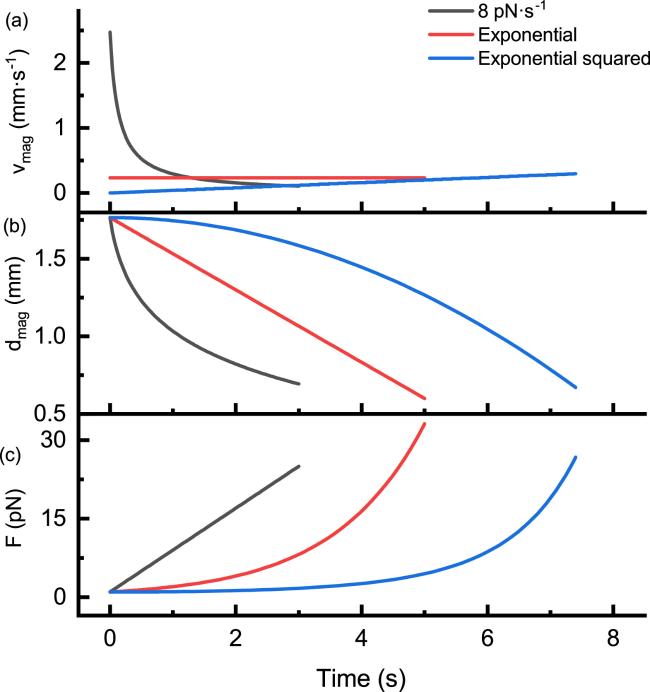
Figure 2. Linear force-loading and two nonlinear force-loading schemes. The plots illustrate the linear force-loading Flinear(t) = 1 + 8t (in black) with a constant loading rate of 8 pN · s−1, the exponential force-loading function ${F}_{\exp }(t)=\exp (0.7t)$ pN (in red) and the exponential squared force-loading function ${F}_{\exp 2}(t)=\exp (0.06{t}^{2})$ pN (in blue). The velocity of magnets (a), the distance between the magnets and the sample (b), and force (c) are shown as functions of time for three types of force-loading schemes. |
We calculated the velocity profile of magnets vmag(t) [figure 2(a)], and the trajectory of magnets dmag(t) [figure 2(b)] in the MT setup for these three types of F(t). Under linear force-loading, the magnets move with drastically changing velocity, especially with high velocity and high acceleration at lower forces. The motion of the magnets under the exponential force-loading is slower with constant velocity. Under the exponential squared force-loading, the magnets move with constant acceleration. Therefore, the exponential force-loading offers a more user-friendly control, requiring only motion with uniform velocity.
Furthermore, we examined the unfolding force distributions P(F) under these three types of force-loading. We derived the formula for P(F) and performed numerical calculations [figures 3(a)–(c)]. Based on equation (5 ), the unfolding force distribution for the linear force-loading function (2 ) is given by,3 ) is given by,
$\begin{eqnarray}\begin{array}{l}{P}_{\mathrm{linear}}(F)=\displaystyle \frac{{k}_{0}}{r}\exp \left[\beta {x}_{{\rm{u}}}F-\displaystyle \frac{{k}_{0}}{\beta {x}_{{\rm{u}}}r}\left(\exp (\beta {x}_{{\rm{u}}}F)\right.\right.\\ \quad \left.\left.\,-\,\exp (\beta {x}_{{\rm{u}}}{F}_{0})\right)\right].\end{array}\end{eqnarray}$
The unfolding force distribution for the exponential force function ( $\begin{eqnarray}\displaystyle \begin{array}{l}{P}_{\exp }(F)=\frac{{k}_{0}}{{v}_{0}F}\exp \left[\beta {x}_{{\rm{u}}}F-\frac{{k}_{0}}{{v}_{0}}(\mathrm{Ei}(\beta {x}_{{\rm{u}}}F)\right.\\ \quad \left.\,-\,\mathrm{Ei}(\beta {x}_{{\rm{u}}}{F}_{0}))\right],\end{array}\end{eqnarray}$
where Ei(x) represents the exponential integral function: $\begin{eqnarray}\mathrm{Ei}(x)={\int }_{-\infty }^{x}\displaystyle \frac{{{\rm{e}}}^{t}}{t}{\rm{d}}t.\end{eqnarray}$
For the exponential squared force function, we cannot derive the analytical formula of unfolding force distribution, while the numerical solution can be obtained.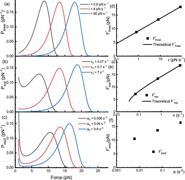
Figure 3. The unfolding force distribution for linear force-loading and two nonlinear force-loading schemes following Bell’s model. (a) The unfolding force distributions under linear force-loading with constant loading rates r = 0.8 (black), 8 (red) and 80 (blue) pN · s−1. (b) The unfolding force distributions for the exponential force-loading function with parameters v0 = 0.07 (black), 0.7 (red) and 7 (blue) s−1. (c) The unfolding force distributions for the exponential squared force-loading function with parameters a0 = 0.006 (black), 0.06 (red) and 0.6 (blue) s−2. (d) The relationship between the most probable force ${F}_{\mathrm{linear}}^{* }$ and loading rate r under linear force-loading. The square dots are derived from the numerical data in figure (a), and the black line represents the theoretical relationship. (e) The relationship between the most probable force ${F}_{\exp }^{* }$ and parameter v0 for the exponential force-loading. The square dots are derived from numerical data in (b), and the black line represents the theoretical relationship. (f) The relationship between the most probable force ${F}_{\exp 2}^{* }$ and parameter a0 for the exponential squared force-loading. The square dots are derived from numerical data in (c). |
We conducted numerical calculations of the probability density of unfolding force for different parameters. For each of the three force functions, three sets of parameters were used to calculate unfolding force distributions P(F) [figures 3(a)–(c)]. The parameters for the red curve are the same as in figure 2.
Under linear force-loading, it was observed that the shape of P(F) remains essentially the same across different loading rates, with the most probable unfolding force (${F}_{\mathrm{linear}}^{* }$) increasing with the loading rate [figure 3(a)]. Similarly, for both exponential and exponential squared force functions, the most probable unfolding forces (${F}_{\exp }^{* }$, ${F}_{\exp 2}^{* }$) increase with the parameters v0 or a0 [figures 3(b) and (c)].
For the linear force-loading, the Bell–Evans formula provides the relationship between the most probable unfolding force ${F}_{\mathrm{linear}}^{* }$ and the loading rate r [13]:
$\begin{eqnarray}\displaystyle \frac{{k}_{0}}{\beta {x}_{{\rm{u}}}}\exp (\beta {x}_{{\rm{u}}}{F}_{\mathrm{linear}}^{* })=r,\end{eqnarray}$
which gives: $\begin{eqnarray}{F}_{\mathrm{linear}}^{* }=\displaystyle \frac{1}{\beta {x}_{{\rm{u}}}}\mathrm{ln}\left(\displaystyle \frac{\beta {x}_{{\rm{u}}}r}{{k}_{0}}\right).\end{eqnarray}$
We computed the relationship between the most probable unfolding force (${F}_{\exp }^{* }$) and the force-loading parameter v0 under Bell’s model for the exponential force function:
$\begin{eqnarray}\displaystyle \frac{{k}_{0}}{\beta {x}_{{\rm{u}}}{F}_{\exp }^{* }-1}\exp (\beta {x}_{{\rm{u}}}{F}_{\exp }^{* })={v}_{0},\end{eqnarray}$
whose solution is expressed with a Lambert W function Wk(z) [24]: $\begin{eqnarray}{F}_{\exp }^{* }({v}_{0})=\displaystyle \frac{1-{W}_{k}(-{\rm{e}}{k}_{0}/{v}_{0})}{\beta {x}_{{\rm{u}}}}.\end{eqnarray}$
When dealing exclusively with real numbers, it suffices to consider W−1 and W0. Here, W−1 corresponds to the maxima in the unfolding force distribution profile, while W0 corresponds to the minima. According to the probability distribution [figure 3(b)], the smaller solution W0 corresponds to a local minimum of the probability distribution function, consistent with the upward trend in probability at lower forces observed in the exponential force-loading.We plotted the analytical relationships [figures 3(d)–(f)] of the most probable force F* with the force-loading parameters (equations (12 ) and (14 )) and compared them with specific points of the most probable force derived from the numerical probability distribution P(F) [figures 3(a)–(c)]. It is concluded that F* derived numerically for the linear force-loading and exponential force-loading curves are consistent with the predictions of analytical equations (12 ) and (14 ) [figures 3(d)–(e)].
For the case of an exponential squared force-loading, the unfolding probability distribution ${P}_{\exp 2}(F)$ resists simplification, and the most probable unfolding force ${F}_{\exp 2}^{* }$ is challenging to calculate. Although no specific analytical expression has been derived, the scatter plot from the numerical method suggests that ${F}_{\exp 2}^{* }$ is also approximately a linear function of the logarithm of a0.
At lower forces, both the exponential and exponential squared force functions show more unfolding events, especially the exponential squared force-loading, which exhibits a pronounced upward trend at very low forces. This phenomenon is more evident when the force-loading parameters (v0 or a0) are small, which is related to the longer duration these functions spend at lower forces.
3.2. Practicality comparison of exponential force functions
Our focus was directed towards the study of exponential force functions, due to their ease of implementation in magnetic tweezers setups. We compared the unfolding events obtained under constant loading rate, exponential loading and exponential squared loading conditions [figure 4]. The force curves for these three conditions are as shown in figure 2(c). The peak distributions of unfolding events for all three force-loading functions are closely aligned (around 14 pN). At lower forces, the exponential and exponential squared functions exhibit more unfolding events, especially the exponential squared function, which shows a pronounced upward trend at very low forces. The upward trend observed in the probability density curves is not always present. Through analytical derivation, we found that under the exponential force-loading, the occurrence of a local minimum requires the exponential function parameter F0 to be sufficiently small (preferably less than 1/βxu), and v0 to satisfy the inequality v0 > k0e2. Moreover, the probability density curves for the exponential and exponential squared force-loading functions appear flatter. For example, the probability at 2.5 pN differs by approximately a factor of 10. Under the exponential function, the magnets in our setup required only a uniform motion and remained at low speeds over an extended period [figure 2(a)], offering mechanical stability far surpassing that under the constant loading rate. Thus, the exponential force-loading function not only facilitates easier implementation in experimental setups but also fully meets the requirements for standard measurements of protein unfolding events.
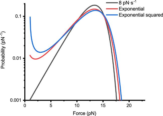
Figure 4. Under Bell’s model, when the forces involved in protein unfolding events are approximately similar, we present a comparative graph of the theoretical probability density P(F) distributions for unfolding events under linear, exponential and exponential squared force-loading. The specific force functions are Flinear(t) = 1 + 8t (in black), ${F}_{\exp }(t)=\exp (0.7t)$ pN (in red) and ${F}_{\exp 2}(t)=\exp (0.06{t}^{2})$ pN (in blue). The three curves in the graph represent the numerical solutions for the theoretical probability density P(F), calculated using these three force curves F(t) and typical protein molecular properties, with 1000 equidistant numerical solutions for each curve. |
3.3. Derivation of F(t) to generate uniform P(F)
According to the Dudko–Hummer–Szabo equation, ku(F) can be obtained in the force range with a non-zero histogram, and the relative error depends on the counts of unfolding events in each bin. Therefore, we raise the question: what kind of force-loading function can generate a uniformly distributed F? With uniformly distributed F, the rate of change of survival probability is proportional to the rate of change of F:
$\begin{eqnarray}{k}_{{\rm{u}}}(F(t))S(t)={C}_{0}\displaystyle \frac{{\rm{d}}F(t)}{{\rm{d}}t},\end{eqnarray}$
where C0 is a proportionality constant, and $\begin{eqnarray}S(t)=\exp \left(-{\int }_{0}^{t}{k}_{{\rm{u}}}(F(t^{\prime} )){\rm{d}}t^{\prime} \right).\end{eqnarray}$
Combining equations (1 ), (15 ) and (16 ), we derived the following relationship:Appendix ].
$\begin{eqnarray}t(F)=-\displaystyle \frac{1}{{k}_{{\rm{u}}}({F}_{0})}\mathrm{Ei}\left(\beta ({F}_{0}-F(t)){x}_{{\rm{u}}}\right)+{t}_{0},\end{eqnarray}$
where t(F) is the inverse function of F(t), and F0 and t0 are constants of integration that incorporate the constant C0 and the force range with uniform distribution [Directly deriving the expression for F(t) is challenging. Therefore, F(t) is obtained using the numerical method. The exponential integral Ei(x) diverges as x → 0, and its inverse function has multiple-value regions. Consequently, F(t) theoretically possesses two distinct solutions satisfying the equation; one solution of F1(t) increases with time, while the other solution F2(t) decreases with time [figure 5(a)].
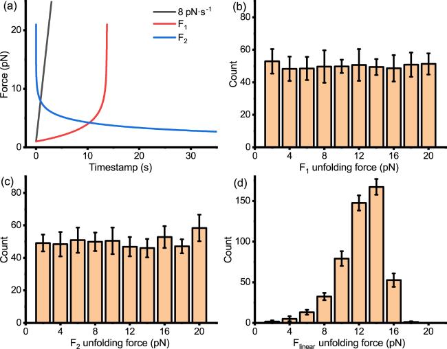
Figure 5. Visualization of the force curves for force-loading F1/2(t) that can uniformly distribute the unfolding force and linear force-loading. Histogram of simulated unfolding events with respect to force under these conditions. (a) The force curves observed in the range of 1–21 pN generated by proteins with typical attributes. The red and blue curves represent monotonically increasing and decreasing forces, respectively, generated using the inverse function of equation ( |
Having obtained F1(t) and F2(t) force curves that can uniformly distribute the unfolding force within the range of 1–21 pN through equation (17 ), we tested the unfolding force distributions of protein under this force-loading via Monte Carlo simulation [figures 5(b)–(c)], which are significantly flatter than the unfolding force distributions under linear force-loading [figure 5(d)]. Under F1(t) or F2(t) force-loading, the unfolding force distributions cover our range of interest (1–21 pN) and are nearly flat, fulfilling the initial assumption.
In F1(t) or F2(t) force-loading curves, the absolute value of the slope is exceptionally high, specifically during the late phase of the monotonically increasing curve F1(t) and the early phases of the monotonically decreasing curve F2(t) [figure 5(a)]. Insufficient density of sampling data points in single-molecule manipulation experiment setups can lead to significant precision loss. Under the monotonically decreasing F2(t) force-loading, there is a steeper slope at the beginning of the experiment and a more extended duration of low force at the end of the experiment. In addition, starting from a high force is not easy to control in magnetic tweezers experiments. Therefore, only F1(t) might be practical in real experiments.
4. Summary and discussion
Theoretically, the force-loading function F(t), force-dependent transition rate ku(F) and unfolding force distribution P(F) are interdependent. With two of them known, the third can be obtained. In single-molecule manipulation experiments, we set F(t), measure P(F) and analyze the data to obtain ku(F).
In traditional single-molecule manipulation experiments, linear force-loading with a constant loading rate is the most popular approach. Constant force measurement can be considered as zero loading rate, which gives the transition rate at a specific force. In this study, we have explored several typical nonlinear force-loading methods. The force of magnetic tweezers is almost an exponential function of the distance between the magnets and the sample. Consequently, we analyzed the distribution of protein unfolding forces under exponential and exponential squared force-loading functions, corresponding to the movements of magnets with constant velocity and constant acceleration, respectively. We found that the obtained force distribution is broader compared to constant loading rate measurements, providing unfolding rates across a larger force range.
We found that exponential force-loading provides an additional advantage when it is used in magnetic tweezers. Under similar forces, the motion of the magnet using exponential force-loading involves slower velocities and smaller accelerations compared to the constant loading rate. This offers greater mechanical stability for the experimental apparatus. On the other hand, with the same limitation of velocity and acceleration, exponential force-loading can cover a larger range of dynamic measurements, which is important since it reveals the more detailed free-energy landscape of biomolecules.
In addition, we have conducted theoretical analyses with the premise of uniformly distributed unfolding force across a certain force range. We have derived the force function F(t) under Bell’s model to meet this expectation. Surprisingly, we discovered a force curve that decreases monotonically over time and also meets our expectation of uniform force distribution. Although it might be not very practical in experiments since we do not know ku(F) in advance, as the first trial to derive force function F(t) with known ku(F) and P(F), this demonstrates that there are two solutions of F(t) that both satisfy the requirements.
In magnetic tweezers experiments, the extension of molecule is obtained from the position of the magnetic bead. When the fluctuation of the extension is much smaller than the unfolding step size, the unfolding event can be identified accurately. Force is only determined by the distance between the permanent magnets and the sample. Therefore, the uncertainty of unfolding force is affected by the synchronization of the camera and the position reading of the motorized stage that moves magnets in the setup. Fortunately, the uncertainty of the unfolding force for each unfolding event is usually much smaller than the distribution range of the unfolding forces. Therefore, noise of both force and extension will not affect the application of our theoretical results in magnetic tweezers experiments.
Acknowledgments
This research project was supported by the National Natural Science Foundation of China (Grant Nos. 12174322 to HC, 12204124 to ZG, 32271367 and 12204389 to SL), the 111 project (Grant No. B16029) and the Research Fund of Wenzhou Institute.
Appendix: Derivation of nonlinear F(t) for uniform P(F) under Bell’s model
This section gives the derivation procedures of equation (17 ). With uniform P(F), equation (15 ) and the following two equations:A1 ) into Bell’s model (1 ), we get:A4 ) into equation (A3 ) yields:10 )), we can determine that,A4 ), we obtain:17 ).
$\begin{eqnarray}\frac{{\rm{d}}F(t)}{{\rm{d}}t}=-k(t)(F(t)+{F}_{0}),\end{eqnarray}$
and $\begin{eqnarray*}S(t)={C}_{1}F(t)+{C}_{2},\end{eqnarray*}$
are equivalent, where F0, C1 and C2 are constants of integration. These equations essentially state that S(t) and F(t) are linearly related at any time. By inserting equation ( $\begin{eqnarray}\displaystyle \frac{{\rm{d}}F(t)}{{\rm{d}}t}=-\exp (\beta {x}_{{\rm{u}}}F(t))({k}_{0}F(t)+{C}_{3}),\end{eqnarray}$
where C3 is a constant of integration. After transformation, we obtain: $\begin{eqnarray}\begin{array}{l}\displaystyle \frac{\exp (-\beta {x}_{{\rm{u}}}{C}_{3}/{k}_{0}-\beta {x}_{{\rm{u}}}F(t))}{-\beta {x}_{{\rm{u}}}{C}_{3}/{k}_{0}-\beta {x}_{{\rm{u}}}F(t)}(-\beta {x}_{{\rm{u}}})\\ \quad \times \displaystyle \frac{{\rm{d}}F(t)}{{\rm{d}}t}=-{k}_{0}\exp \left(-\displaystyle \frac{\beta {x}_{{\rm{u}}}{C}_{3}}{{k}_{0}}\right).\end{array}\end{eqnarray}$
Let us define: $\begin{eqnarray}g(t)=-\beta {x}_{{\rm{u}}}{C}_{3}/{k}_{0}-\beta {x}_{{\rm{u}}}F(t),\end{eqnarray}$
Substituting equation ( $\begin{eqnarray*}\displaystyle \frac{\exp (g(t))}{g(t)}\displaystyle \frac{{\rm{d}}g(t)}{{\rm{d}}t}=-{k}_{0}\exp \left(-\displaystyle \frac{\beta {x}_{{\rm{u}}}{C}_{3}}{{k}_{0}}\right).\end{eqnarray*}$
Moreover, considering the expression for Ei (equation ( $\begin{eqnarray}\displaystyle \frac{\mathrm{dEi}[g(t)]}{{\rm{d}}t}=\displaystyle \frac{\exp (g(t))}{g(t)}\displaystyle \frac{{\rm{d}}g(t)}{{\rm{d}}t}.\end{eqnarray}$
Thus, it can be concluded that, $\begin{eqnarray*}\displaystyle \frac{\mathrm{dEi}[g(t)]}{{\rm{d}}t}=-{k}_{0}\exp \left(-\displaystyle \frac{\beta {x}_{{\rm{u}}}{C}_{3}}{{k}_{0}}\right).\end{eqnarray*}$
Integrating both sides results in the following: $\begin{eqnarray*}\mathrm{Ei}[g(t)]=-{k}_{0}\exp \left(-\displaystyle \frac{\beta {x}_{{\rm{u}}}{C}_{3}}{{k}_{0}}\right)t+{C}_{4},\end{eqnarray*}$
where C4 is a constant of integration. After simplification, we have: $\begin{eqnarray*}-\displaystyle \frac{\exp (\beta {x}_{{\rm{u}}}{C}_{3}/{k}_{0})\mathrm{Ei}[g(t)]}{{k}_{0}}=t+{C}_{5},\end{eqnarray*}$
where C5 is another constant of integration. Substituting with equation ( $\begin{eqnarray*}-\displaystyle \frac{\exp (\beta {x}_{{\rm{u}}}{C}_{3}/{k}_{0})\mathrm{Ei}(-\beta {x}_{{\rm{u}}}{C}_{3}/{k}_{0}-\beta {x}_{{\rm{u}}}F(t))}{{k}_{0}}=t+{C}_{5}.\end{eqnarray*}$
After further simplification, we obtain equation (