


1. Introduction
Resistor networks are important models in engineering and natural sciences, and the calculation of resistance between two nodes is a classical problem in the fields of circuit theory, the research of which has exceeded 180 years [1–3]. At present, new breakthroughs have been made in resistor network research [1–4]. The breakthrough in resistor network theory is very important, and its research theory can be applied to study complex impedance networks and fractional-order circuits (FOCs) through variable substitution. As is known, circuit network theory is very closely related to our lives, and it can help us solve many practical problems encountered in real life [5–9]. Because of its flexibility, fractional-order (FO) theory has been widely used in applied physics, biology, mathematics, engineering and other fields, and has a close relationship with all areas of our lives [10–23].
The study of fractional calculus has been going on for hundreds of years, but the real application of fractional calculus to modern fields is due to the great progress in the research in recent decades [24]. Reference [25] tells us that the ubiquitous FO capacitors have become the new norm and open a new era of fractional calculus and its engineering applications. Reference [26] researched fractional-order inductors, which can be designed based on skin effects. Nowadays, with increasing new phenomena, new laws and new applications of components, researchers need to constantly solve new problems [27–29]. References [30–33] have had a significant impact on the definition and research of fractional calculus. In recent years, a number of researchers have devoted themselves to the study of FOC theory [34–37]; among them, some of the literature focuses on physical analysis [34], some focus on circuit models [35], while others focus on mathematical analysis [36, 37]. Researchers have found that the study of FOCs can be directly implemented using resistor network theory, and numerous studies have made many achievements in the study of resistor network models. For example, [3, 4] set up the RT-I theory, while [38] set up the RT-V theory. These theories provide new a theoretical basis for studying resistor network models with various complex boundaries, such as in [4, 38–46]. In addition, Green’s function technology has played an important role in the study of infinite networks, such as in [1, 47–50]. In [47], Owaidat used Green’s function method to study infinite resistance networks of the ruby lattice structure. References [48, 49] studied the equivalent resistance and capacitance when one bond is removed from the infinite perfect cubic lattice, while [50] investigated infinite networks with two bonds removed. In summary, Green’s function technology is only applicable to infinite networks; the method established in [2] is called the LM method, which can solve resistor network models with regular boundaries, but cannot be used to study resistor network models with complex boundaries. However, the RT-I [3] and RT-V [38] methods fill this gap.
In this article, RT-I theory [3] is applied to study the electrical characteristics of the FO 3 × n Fan circuit network. First, three general formulae of the impedances for the FO 3 × n Fan network are derived using RT-I theory. Second, from the perspective of the circuit, the amplitude-frequency and phase-frequency characteristics of equivalent complex impedance are studied based on complex analysis and Matlab drawing research in detail. Specifically, the fractional calculus describes the physical phenomena better, which is impossible for the ordinary circuit network. Our research includes various circuit structures, such as RCα circuits, RLβ circuits, LβCα circuits and LC circuits.
This article mainly includes four parts. In section 2 , we mainly introduce some basic definitions of FOCs and three equivalent complex impedance formulae. In section 3 , the expression of equivalent impedance is derived using RT-I theory. In section 4 , amplitude-frequency and phase-frequency characteristics are elucidated by Matlab drawing. In section 5 , we provide a summary of the article.
2. FO definition and impedance formulae
2.1. Definition of fractional capacitor and inductors
So far, the ethics of fractional calculus are satisfied with the unified theory. In the continuous research process, several definitions of fractional calculus (such as Grünwald–Letnikov, Caputo, Riesz, and Riemann–Liouville) have already coexisted [31–33]. Now researchers have applied FO fractional calculus theory to the study of FOCs [34, 35].
The concept of FO in mathematics has been applied in the field of circuits. First, for impedance circuits with an inductor of L and a capacitance of C, the basic relationship between LC, current and voltage is ${i}_{C}=C\tfrac{d{u}_{c}}{dt},$ ${u}_{L}=L\tfrac{d{i}_{L}}{dt}.$ According to fractional calculus theory, a simple integer-order LC circuit can be extended to a fractional structure. For example [30]1 ) has been described in [30]. In particular, when $\alpha =\beta =1,$ equation (1 ) is reduced to an integer-order differential equation.
$\begin{eqnarray}{i}_{C}={C}_{\alpha }\displaystyle \frac{{{\rm{d}}}^{\alpha }{u}_{c}}{{\rm{d}}{t}^{\alpha }},\,{u}_{L}={L}_{\beta }\displaystyle \frac{{{\rm{d}}}^{\beta }{i}_{L}}{{\rm{d}}{t}^{\beta }},\end{eqnarray}$
where $0\leqslant \alpha \leqslant 1,\,0\leqslant \beta \leqslant 1.$ Equation (According to the research from [30, 34], the FO capacitance and inductance functions can be expressed as
$\begin{eqnarray*}{Z}_{C}=\displaystyle \frac{1}{{\omega }^{\alpha }C}{{\rm{e}}}^{j\left(-\alpha \pi /2\right)}=\displaystyle \frac{1}{{\omega }^{\alpha }C}\,\cos \left(\displaystyle \frac{\alpha \pi }{2}\right)-j\displaystyle \frac{1}{{\omega }^{a}C}\,\sin \left(\displaystyle \frac{\alpha \pi }{2}\right),\end{eqnarray*}$
$\begin{eqnarray}{Z}_{L}={\omega }^{\beta }L{{\rm{e}}}^{j\left(\beta \pi /2\right)}={\omega }^{\beta }L\,\cos \left(\displaystyle \frac{\beta \pi }{2}\right)+j{\omega }^{\beta }L\,\sin \left(\displaystyle \frac{\beta \pi }{2}\right),\end{eqnarray}$
where ω is the circular frequency of alternating current. Obviously, the impedance of a fractional ${L}_{\beta }{C}_{\alpha }$ circuit involves many parameters.The physical meaning of the fractional-order circuit has been discussed in [29, 30, 34], and here we will present some simple understandings. For example, taking a fractional-order capacitor network as an example, its complex impedance is the first equation in the equation system (2), when α = 0, there will be $Z=1/C$, which is a real number; it shows pure resistance properties, and we study it as a pure resistance circuit. When α = 1, there will be $Z=-j/\left(\omega C\right)$, which is a purely imaginary number, i.e. it exhibits ideal pure capacitance properties. When α = 1/2, there will be $Z\,=1/\left(C\sqrt{2\omega }\right)-j/\left(C\sqrt{2\omega }\right)$, which is a complex impedance containing real and imaginary parts, i.e. it is a circuit composed of resistance and capacitance. The actual capacitance is indeed a complex impedance with real and imaginary parts [6–21, 30] (e.g. α = 0.8); as a theoretical study, we can extend the range of α values to $0\leqslant \alpha \leqslant 1.$ The influence of these multiple parameters on the circuit will be studied and discussed below.
2.2. Equivalent complex impedance formulae
This article focuses on the equivalent complex impedance of a class of FO 3 × n ${L}_{\beta }{C}_{\alpha }$ Fan network shown in figure 1. The meaning of the Fan network is that the resistance of the lower boundary is zero, which can be topologically a node O [38]; therefore, we can unify the entire lower boundary with a node O. The fractional elements in figure 1 are designed as follows: fractional inductive elements ${Z}_{L}\left(\omega ,\beta \right)$ on the horizontal axis, and fractional capacitive elements ${Z}_{C}(\omega ,\alpha )$ on the vertical axis. The circular frequency ω of the alternating current passes into the circuit; then the equivalent complex impedance between any node ${A}_{{\rm{x}}},$ ${B}_{{\rm{x}}},$ ${C}_{{\rm{x}}}$( here, $x\in [0,n]$ is an arbitrary integer ) and node O, respectively, are
$\begin{eqnarray}{Z}_{{A}_{{\rm{x}}}O}(n)=\displaystyle \frac{2}{7}\left[\displaystyle \frac{{{\rm{e}}}^{-j\alpha \pi /2}}{{\omega }^{\alpha }C}\right]\displaystyle \sum _{i=1}^{3}\displaystyle \frac{{\rm{\Delta }}{F}_{x}^{(i)}{\rm{\Delta }}{F}_{n-x}^{(i)}}{{F}_{n+1}^{(i)}}\displaystyle \frac{{\sin }^{2}(3{\theta }_{i})}{1-\,\cos \,{\theta }_{i}},\end{eqnarray}$
$\begin{eqnarray}{Z}_{{B}_{x}O}(n)=\displaystyle \frac{2}{7}\left[\displaystyle \frac{{{\rm{e}}}^{-j\alpha \pi /2}}{{\omega }^{\alpha }C}\right]\displaystyle \sum _{i=1}^{3}\displaystyle \frac{{\rm{\Delta }}{F}_{x}^{(i)}{\rm{\Delta }}{F}_{n-x}^{(i)}}{{F}_{n+1}^{(i)}}\displaystyle \frac{{\sin }^{2}(2{\theta }_{i})}{1-\,\cos \,{\theta }_{i}},\end{eqnarray}$
$\begin{eqnarray}{Z}_{{C}_{x}O}(n)=\displaystyle \frac{2}{7}\left[\displaystyle \frac{{e}^{-j\alpha \pi /2}}{{\omega }^{\alpha }C}\right]\displaystyle \sum _{i=1}^{3}\displaystyle \frac{{\rm{\Delta }}{F}_{x}^{(i)}{\rm{\Delta }}{F}_{n-x}^{(i)}}{{F}_{n+1}^{(i)}}\displaystyle \frac{{\sin }^{2}({\theta }_{i})}{1-\,\cos \,{\theta }_{i}},\end{eqnarray}$
where some relevant parameters are defined as follows: $\begin{eqnarray}{F}_{k}^{(i)}=\left({\lambda }_{i}^{k}-{\bar{\lambda }}_{i}^{k}\right)/\left({\lambda }_{i}-{\bar{\lambda }}_{i}\right),\,{\rm{\Delta }}{F}_{k}^{(i)}={F}_{k+1}^{(i)}-{F}_{k}^{(i)},\end{eqnarray}$
with $\begin{eqnarray*}{\lambda }_{i}=1+p-p\,\cos \,{\theta }_{i}+\sqrt{{(1+p-p\,\cos \,{\theta }_{i})}^{2}-1},\end{eqnarray*}$
$\begin{eqnarray}{\bar{\lambda }}_{i}=1+p-p\,\cos \,{\theta }_{i}-\sqrt{{(1+p-p\,\cos \,{\theta }_{i})}^{2}-1},\end{eqnarray}$
$\begin{eqnarray}{\theta }_{i}=\left(2i-1\right)\pi /7,\,p={Z}_{L}/{Z}_{C}=LC{\omega }^{\left(\alpha +\beta \right)}{{\rm{e}}}^{j\displaystyle \frac{\pi }{2}\left(\alpha +\beta \right)}.\end{eqnarray}$
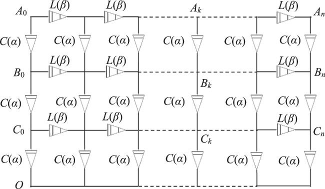
Figure 1. The FO 3 × n Fan circuit network model; fractional inductive elements ZL(ω,β),are arranged on the horizontal axis, and fractional capacitor elements ZC(ω,α) are arranged on the vertical axis. |
The above are the analytic expression of equivalent complex impedance for the FO 3 × n ${L}_{\beta }{C}_{\alpha }$ circuit established in this article. Below, we first give the derivation and calculation of the above results; the Matlab drawing tool is used to plot the images of the equivalent complex impedance ${Z}_{{A}_{{\rm{x}}}O}(n)$ changing with the circular frequency ω of alternating current and the node position x. Therefore, the amplitude-frequency and phase-frequency characteristics of the equivalent complex impedance ${Z}_{{A}_{{\rm{x}}}O}(n)$ are fully understood by visual methods.
3. Derivation and calculation of main results
3.1. Construction of the difference equation model
An FO 3 × n Fan circuit network in the topology is shown in figure 2, where the current J is input from an arbitrary node ${A}_{x}$(or ${B}_{x},$ ${C}_{x}$) and the output is from the lower boundary of O. For ease of study, we re-represent the resistor network shown in figure 1 as the circuit network graph with current parameters and their direction shown in figure 2. The currents passing through the resistors of the three horizontal axes are ${I}_{ak},$ ${I}_{bk}$ and ${I}_{ck}$ ($1\leqslant k\leqslant n$), respectively. The currents passing through the longitudinal impedance ${Z}_{C}(\omega ,\alpha )$ are ${I}_{k}^{(1)},$ ${I}_{k}^{(2)}$ and ($0\leqslant k\leqslant n$), respectively.
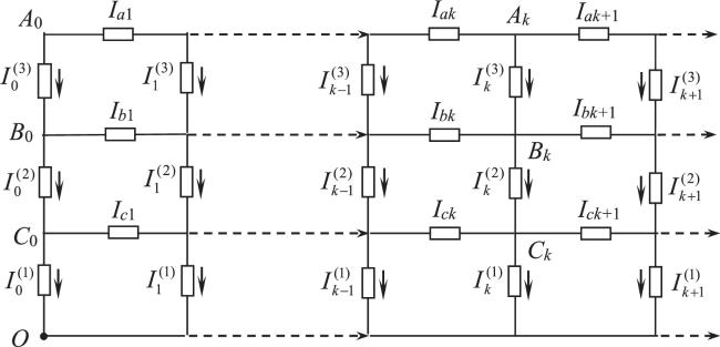
Figure 2. The topology of the FO 3 × n Fan network and its parameter assumption simplified circuit model with the direction of the current parameters. |
This paper mainly adopts RT-I theory [4] to carry out research. We first derive the equivalent complex impedance ${Z}_{{A}_{{\rm{x}}}O}(n),$ for this reason, and assume that current J flows in from node ${A}_{{\rm{x}}}$ and then flows out from point O. According to the network analysis, the loop voltage equation of the kth grid is obtained
$\begin{eqnarray}{I}_{k}^{(1)}{Z}_{C}-{I}_{k-1}^{(1)}{Z}_{C}+{I}_{k}^{(c)}{Z}_{L}=0,\end{eqnarray}$
$\begin{eqnarray}{I}_{k}^{(2)}{Z}_{C}-{I}_{k-1}^{(2)}{Z}_{C}+{I}_{k}^{(b)}{Z}_{L}-{I}_{k}^{(c)}{Z}_{L}=0,\end{eqnarray}$
$\begin{eqnarray}{I}_{k}^{(3)}{Z}_{C}-{I}_{k-1}^{(3)}{Z}_{C}+{I}_{k}^{(a)}{Z}_{L}-{I}_{k}^{(b)}{Z}_{L}=0.\end{eqnarray}$
The nodal current equation is obtained according to figure 2 $\begin{eqnarray}{I}_{k}^{(c)}-{I}_{k+1}^{(c)}={I}_{k}^{(1)}-{I}_{k}^{(2)},\end{eqnarray}$
$\begin{eqnarray}{I}_{k}^{(b)}-{I}_{k+1}^{(b)}={I}_{k}^{(2)}-{I}_{k}^{(3)},\end{eqnarray}$
$\begin{eqnarray}{I}_{k}^{(a)}-{I}_{k+1}^{(a)}={I}_{k}^{(3)}-{\delta }_{k,x}J.\end{eqnarray}$
Similar to the establishment of equations (9 )–(11 ), the loop voltage equation of the $k+1$ grid can be set up. Then, using equations of the $k+1$ grid together with (9 )–(11 ) and (12 )–(14 ), we can obtain an equation system containing only the vertical current,15 ) as a matrix17 ). First, let the eigenvalue of the matrix in equation (17) be ${t}_{1},{t}_{2},{t}_{3}.$ The third-order determinant is used18 ) to get (one can refer to [3])
$\begin{eqnarray*}{I}_{k+1}^{(1)}=(2+p){I}_{k}^{(1)}-{I}_{k-1}^{(1)}-p{I}_{k}^{(2)},\end{eqnarray*}$
$\begin{eqnarray*}{I}_{k+1}^{(2)}=(2+2p){I}_{k}^{(2)}-{I}_{k-1}^{(2)}-p{I}_{k}^{(1)}-p{I}_{k}^{(3)},\end{eqnarray*}$
$\begin{eqnarray}{I}_{k+1}^{(3)}=(2+2p){I}_{k}^{(3)}-{I}_{k-1}^{(3)}-p{I}_{k}^{(2)}-Jp{\delta }_{k,x},\end{eqnarray}$
where $p={Z}_{L}/{Z}_{C},$ represents the system of equation ( $\begin{eqnarray}\left[\begin{array}{c}{I}_{k+1}^{(1)}\\ {I}_{k+1}^{(2)}\\ {I}_{k+1}^{(3)}\end{array}\right]={A}_{3\times 3}\left[\begin{array}{c}{I}_{k}^{(1)}\\ {I}_{k}^{(2)}\\ {I}_{k}^{(3)}\end{array}\right]-\left[\begin{array}{c}{I}_{k-1}^{(1)}\\ {I}_{k-1}^{(2)}\\ {I}_{k-1}^{(3)}\end{array}\right]-\left[\begin{array}{c}0\\ 0\\ Jp\end{array}\right]{\delta }_{k,x},\end{eqnarray}$
and ${A}_{3\times 3}$ is a third-order matrix $\begin{eqnarray}{A}_{3\times 3}=\left(\begin{array}{ccc}2+p & -p & 0\\ -p & 2+2p & -p\\ 0 & -p & 2+2p\end{array}\right).\end{eqnarray}$
The matrix transform method set up in [3, 4] is applied to the third-order matrix of equation ( $\begin{eqnarray}\det \left|{A}_{3\times 3}-tE\right|=0,\end{eqnarray}$
solving equation ( $\begin{eqnarray}{t}_{i}=2(1+p)-2p\,\cos \,{\theta }_{i},\,\left(i=1,2,3\right)\end{eqnarray}$
where ${\theta }_{i}=(2i-1)\pi /7.$To transform equation (16 ), assume that there is an unknown third-order square matrix ${P}_{3\times 3},$ and the transformation is as follows20 ) is expanded and solved according to the identity of the left and right sides of the matrix, and we have19 ), and the resulting inverse matrix16 ) can be transformed into a simple matrix equation using the matrix ${P}_{3\times 3}$ left-by-multiplied matrix equation (16 ) and applying equation (20 ),23 ), one can obtain the characteristic equation ${x}^{2}-{t}_{k}x+1=0$ for the difference equation of ${X}_{k}.$ Let the two roots of the characteristic equation be ${\lambda }_{k},{\bar{\lambda }}_{k}$ ($k=1,2$); then the solution can be obtained7 ), proposed above.
$\begin{eqnarray}{P}_{3\times 3}{A}_{3\times 3}=\text{diag}({t}_{1},{t}_{2},{t}_{3}){P}_{3\times 3}.\end{eqnarray}$
Equation ( $\begin{eqnarray}{P}_{3\times 3}=\left(\begin{array}{ccc}\cos \left(\displaystyle \frac{1}{2}{\theta }_{1}\right) & \cos \left(\displaystyle \frac{3}{2}{\theta }_{1}\right) & \cos \left(\displaystyle \frac{5}{2}{\theta }_{1}\right)\\ \cos \left(\displaystyle \frac{1}{2}{\theta }_{2}\right) & \cos \left(\displaystyle \frac{3}{2}{\theta }_{2}\right) & \cos \left(\displaystyle \frac{5}{2}{\theta }_{2}\right)\\ \cos \left(\displaystyle \frac{1}{2}{\theta }_{3}\right) & \cos \left(\displaystyle \frac{3}{2}{\theta }_{3}\right) & \cos \left(\displaystyle \frac{5}{2}{\theta }_{3}\right)\end{array}\right),\end{eqnarray}$
where ${\theta }_{i}=(2i-1)\pi /7$ appears in equation ( $\begin{eqnarray}{P}_{3\times 3}^{-1}=\displaystyle \frac{4}{7}\left(\begin{array}{ccc}\cos \left(\displaystyle \frac{1}{2}{\theta }_{1}\right) & \cos \left(\displaystyle \frac{1}{2}{\theta }_{2}\right) & \cos \left(\displaystyle \frac{1}{2}{\theta }_{3}\right)\\ \cos \left(\displaystyle \frac{3}{2}{\theta }_{1}\right) & \cos \left(\displaystyle \frac{3}{2}{\theta }_{2}\right) & \cos \left(\displaystyle \frac{3}{2}{\theta }_{3}\right)\\ \cos \left(\displaystyle \frac{5}{2}{\theta }_{1}\right) & \cos \left(\displaystyle \frac{5}{2}{\theta }_{2}\right) & \cos \left(\displaystyle \frac{5}{2}{\theta }_{3}\right)\end{array}\right).\end{eqnarray}$
The matrix equation ( $\begin{eqnarray}{X}_{k+1}^{(i)}={t}_{i}{X}_{k}^{(i)}-{X}_{k-1}^{(i)}-{\delta }_{k,x}Jp\,\cos \left(\displaystyle \frac{5}{2}{\theta }_{i}\right),\,\left(i=1,2,3\right)\end{eqnarray}$
where ${X}_{k}^{(i)}$ is defined as $\begin{eqnarray}{\left[{X}_{k}^{(1)}\,{X}_{k}^{(2)}\,{X}_{k}^{(3)}\right]}^{{\rm{T}}}={P}_{3\times 3}{\left[{I}_{k}^{(1)}\,{I}_{k}^{(2)}\,{I}_{k}^{(3)}\right]}^{{\rm{T}}}.\end{eqnarray}$
From equation ( $\begin{eqnarray}{\lambda }_{k}=\displaystyle \frac{1}{2}\left({t}_{k}+\sqrt{{t}_{k}^{2}-4}\right),\,{\bar{\lambda }}_{k}=\displaystyle \frac{1}{2}\left({t}_{k}-\sqrt{{t}_{k}^{2}-4}\right).\end{eqnarray}$
Bringing equation (19) into equation (25) yields equation (According to the method established in [3, 4], solving equation (23 ) to obtain the piecewise functional solution of the difference equation6 ).
$\begin{eqnarray}{X}_{k}^{(i)}={X}_{1}^{(i)}{F}_{k}^{(i)}-{X}_{0}^{(i)}{F}_{k-1}^{(i)}\,\left(0\leqslant k\leqslant x\right),\end{eqnarray}$
$\begin{eqnarray}{X}_{x+1}^{(i)}={t}_{i}{X}_{x}^{(i)}-{X}_{x-1}^{(i)}-Jp\,\cos \left(\displaystyle \frac{5}{2}{\theta }_{i}\right).\end{eqnarray}$
$\begin{eqnarray}{X}_{k}^{(i)}={X}_{x+1}^{(i)}{F}_{k-x}^{(i)}-{X}_{x}^{(i)}{F}_{k-x-1}^{(i)}\,\left(x\leqslant k\leqslant n\right),\end{eqnarray}$
where ${F}_{k}^{(i)}=({\lambda }_{i}^{k}-{\bar{\lambda }}_{i}^{k})/({\lambda }_{i}-{\bar{\lambda }}_{i})$ is defined in equation (3.2. Derivation of the law of boundary current
The boundary current constraint has three parts: namely, the leftmost and rightmost boundary condition constraints, and the boundary condition constraint of the current input node.
Consider the constraint of the left boundary grid. Using a similar method to that used to establish equation (16 ), the matrix equation for the left boundary is obtained according to figure 2 29 ), the matrix equation (29 ) can be converted to
$\begin{eqnarray}{\left[{I}_{1}^{(1)},{I}_{1}^{(2)},{I}_{1}^{(3)}\right]}^{{\rm{T}}}=\left({A}_{3\times 3}-{E}_{3\times 3}\right){\left[{I}_{0}^{(1)},{I}_{0}^{(2)},{I}_{0}^{(3)}\right]}^{{\rm{T}}}.\end{eqnarray}$
If the matrix transformation is implemented to equation ( $\begin{eqnarray}{X}_{1}^{\left(i\right)}=({t}_{i}-1){X}_{0}^{\left(i\right)},\,(i=1,2,3).\end{eqnarray}$
Equation (30 ) is the constraint equation for the left boundary of the FO 3 × n Fan circuit network.
Similarly, the conditional constraint equation for the right boundary of the circuit network can be obtained
$\begin{eqnarray}{X}_{n-1}^{\left(i\right)}=({t}_{i}-1){X}_{n}^{\left(i\right)},\,(i=1,2,3).\end{eqnarray}$
Equation (31 ) is the constraint equation for the right boundary of the FO 3 × n Fan network.
The following is the solution of ${X}_{k}^{(i)}$ according to the above series of equations. Substitute equation (30 ) into equation (26) to simplify27 ), (28 ), (31 ) and (32 ), yielding
$\begin{eqnarray}{X}_{k}^{\left(i\right)}={\rm{\Delta }}{F}_{k}^{\left(i\right)}{X}_{0}^{\left(i\right)}\,\left(0\leqslant k\leqslant x\right).\end{eqnarray}$
It is solved by four equations, ( $\begin{eqnarray}{X}_{k}^{(i)}=Ih\displaystyle \frac{{\rm{\Delta }}{F}_{k}^{(i)}{\rm{\Delta }}{F}_{n-x}^{(i)}}{({t}_{i}-2){F}_{n+1}^{(i)}}\cos \left(\displaystyle \frac{5}{2}{\theta }_{i}\right),\,\left(0\leqslant k\leqslant x\right),\end{eqnarray}$
$\begin{eqnarray}{X}_{k}^{\left(i\right)}=Ih\displaystyle \frac{{\rm{\Delta }}{F}_{x}^{\left(i\right)}{\rm{\Delta }}{F}_{n-k}^{\left(i\right)}}{\left({t}_{i}-2){F}_{n+1}^{\left(i\right)}\right.}\cos \left(\displaystyle \frac{5}{2}{\theta }_{i}\right),\,\left(x\leqslant k\leqslant n\right).\end{eqnarray}$
3.3. Derivation of the equivalent impedance
It is obtained by implementing the inverse matrix transformation according to the matrix in equation (24)33 ) into equation (36) to simplify39 ) into equation (38) to get40 ) into them can be obtained
$\begin{eqnarray}{\left[{I}_{x}^{(1)}\,{I}_{x}^{(2)}\,{I}_{x}^{(3)}\right]}^{{\rm{T}}}={P}_{3\times 3}^{-1}{\left[{X}_{x}^{(1)}\,{X}_{x}^{(2)}\,{X}_{x}^{(3)}\right]}^{{\rm{T}}},\end{eqnarray}$
where ${\left[\cdot \right]}^{T}$ represents the transpose of the matrix. Calculated from equation (35) $\begin{eqnarray}{I}_{x}^{(j)}=\displaystyle \frac{4}{7}\displaystyle \sum _{i=1}^{3}{X}_{x}^{(i)}\cos \left(j-\displaystyle \frac{1}{2}\right){\theta }_{i}.\end{eqnarray}$
Substitute equation ( $\begin{eqnarray}{I}_{x}^{\left(j\right)}=\displaystyle \frac{2I}{7}\displaystyle \sum _{i=1}^{3}\displaystyle \frac{{\rm{\Delta }}{F}_{x}^{\left(i\right)}{\rm{\Delta }}{F}_{n-x}^{\left(i\right)}}{{F}_{n+1}^{\left(i\right)}}\left(\displaystyle \frac{\cos (5{\theta }_{i}/2)\cos (j-1/2){\theta }_{i}}{1-\,\cos \,{\theta }_{i}}\right).\end{eqnarray}$
Referring to figure 2, we can see that ${I}_{k}^{(1)}={I}_{{C}_{k}O},$ ${I}_{k}^{(2)}={I}_{{B}_{k}{C}_{k}}$ and ${I}_{k}^{(3)}={I}_{{A}_{k}{B}_{k}},$ obtained from equation (37) $\begin{eqnarray}\displaystyle \sum _{j=1}^{3}{I}_{x}^{\left(j\right)}=\displaystyle \frac{I}{7}\displaystyle \sum _{i=1}^{3}\displaystyle \frac{{\rm{\Delta }}{F}_{x}^{\left(i\right)}{\rm{\Delta }}{F}_{n-x}^{\left(i\right)}}{{F}_{n+1}^{\left(i\right)}}\displaystyle \frac{\cos \left(5{\theta }_{i}/2\right)}{\left.1-\,\cos ({\theta }_{i}\right)}\displaystyle \frac{\left.\sin (3{\theta }_{i}\right)}{\sin \left({\theta }_{i}/2\right)},\end{eqnarray}$
where it makes use of $\displaystyle {\sum }_{i=1}^{3}\cos \left(j-\displaystyle \frac{1}{2}\right){\theta }_{i}=\displaystyle \frac{1}{2}\,\sin \left(3{\theta }_{i}\right)/\,\sin \left({\theta }_{i}/2\right).$ Since ${\theta }_{i}=(2i-1)\pi /7,$ it gets $\begin{eqnarray}\cos \left(\displaystyle \frac{5}{2}{\theta }_{i}\right)=2\,\sin \left(\displaystyle \frac{{\theta }_{i}}{2}\right)\sin \left(3{\theta }_{i}\right).\end{eqnarray}$
Substitute equation ( $\begin{eqnarray}\displaystyle \sum _{j=1}^{3}{I}_{k}^{(j)}=\displaystyle \frac{2I}{7}\displaystyle \sum _{i=1}^{3}\displaystyle \frac{{\rm{\Delta }}{F}_{x}^{(i)}{\rm{\Delta }}{F}_{n-x}^{(i)}}{{F}_{n+1}^{(i)}}\displaystyle \frac{{\sin }^{2}(3{\theta }_{i})}{1-\,\cos ({\theta }_{i})}.\end{eqnarray}$
As can be seen in figure 2, ${Z}_{{A}_{k}o}(n)={V}_{{A}_{k}}(n)/I$ and ${V}_{{A}_{k}}\left(n\right)=({I}_{k}^{\left(1\right)}+{I}_{k}^{\left(2\right)}+{I}_{k}^{\left(3\right)}){Z}_{C}.$ Substitution of equation ( $\begin{eqnarray}{Z}_{{A}_{{\rm{x}}}O}(n)=\displaystyle \frac{2}{7}\left[\displaystyle \frac{1}{{\omega }^{\alpha }C}{{\rm{e}}}^{j(-\alpha \pi /2)}\right]\displaystyle \sum _{i=1}^{3}\displaystyle \frac{{\rm{\Delta }}{F}_{x}^{(i)}{\rm{\Delta }}{F}_{n-x}^{(i)}}{{F}_{n+1}^{(i)}}\displaystyle \frac{{\sin }^{2}(3{\theta }_{i})}{1-\,\cos \,{\theta }_{i}}.\end{eqnarray}$
So far, we have completely derived the analytical formula for the equivalent complex impedance ${Z}_{{A}_{{\rm{x}}}O}(n),$ where ${A}_{{\rm{x}}}$ is any point on the horizontal axis A0An, so ${Z}_{{A}_{{\rm{x}}}O}(n)$ is a universal formula.In addition, if complex impedances ${Z}_{{B}_{k}O}(n)$ and ${Z}_{{C}_{k}O}(n)$ are calculated, different input nodes of the current need to be considered separately. For example, when calculating complex impedance of ${Z}_{{B}_{k}O}(n),$ it is necessary to consider the current input from ${B}_{x};$ when calculating complex impedance of ${Z}_{{C}_{k}O}(n),$ it is necessary to consider the current input from ${C}_{x}.$ Then, we use the same method as for the calculation of ${Z}_{{A}_{k}O}(n)$ so that we can derive the impedance ${Z}_{{B}_{k}O}(n)$ and ${Z}_{{C}_{k}O}(n).$ The calculation is omitted here.
4. Impedance characteristics of FOC
In this part, we will use the Matlab plotting tool to explore in detail the characteristics of amplitude-frequency and phase-frequency on equivalent complex impedance ${Z}_{AO}(n),$ and to be able to visualize their electrical characteristics. The electrical characteristics of the FOC are very rich, and the change in coefficient $\alpha ,\beta $ has a great influence on the amplitude-frequency and phase-frequency characteristics of ${Z}_{AO}(n).$
To facilitate research and comparison, the relevant parameters in this article are uniformly valued: $n=50,$ $L=0.02,$ $C=0.01,$ $\alpha =0\sim 1.0,$ $\beta =0\sim 1.0.$ The following research is divided into two parts; the first part studies the change law of mode $\left|{Z}_{AO}(x,\omega )\right|$ of complex impedance with the circle frequency ω and different positions x. Part two studies the change law of phase $\phi [{Z}_{AO}(x,\omega )]$ of complex impedance with circular frequency ω and different positions x.
4.1. Visualized amplitude-frequency characteristics
Case 1. Amplitude-frequency characteristic image when α = β = 0.5
To clearly display the amplitude-frequency characteristics at $\alpha =\beta =0.5,$ we consider the significant difference in variation at $\omega =1\sim 10,$ and we divide $\omega =1\sim 100$ into $\omega =1\sim 20$ and $\omega =20\sim 100$ for plotting studies. In the complex impedance ${Z}_{AO}(x,\omega ),$ the x in the image is the coordinate of any point on the horizontal axis A0An, and ω is the circular frequency of the alternating current of the input circuit.
Figure 3 takes the value of n = 50, $L=0.02,$ $C=0.01,$ $\alpha =\beta =0.5,$ and divides ω into $\omega =1\sim 20$ and $\omega =20\sim 100$ for drawing. Take $x=0\to 30$ in the image; specifically, the 3D image drawn represents the amplitude-frequency characteristics of 31 complex impedances. Figure 3(a) shows that $\left|{Z}_{AO}(x,\omega )\right|$ changes significantly when $\omega =1\sim 10,$ and its corresponding $\left|{Z}_{AO}(x,\omega )\right|$ decreases as ω increases. Figure 3(b) shows that when $\omega \geqslant 20$ increases with ω, its corresponding $\left|{Z}_{AO}(x,\omega )\right|$ does not change significantly. Then, we observe the law of change between $\left|{Z}_{AO}(x,\omega )\right|$ and x. Figure 3(a) shows that $\left|{Z}_{AO}(x,\omega )\right|$ hardly changes as x increases when $\omega =1.$ When $\omega =10$ is present, $\left|{Z}_{AO}(x,\omega )\right|$ decreases as x increases. Figure 3(b) shows that when $\omega \gt 20,$ for a definite ω value, between $x=15\to 30,$ its corresponding $\left|{Z}_{AO}(x,\omega )\right|$ does not change significantly with the change in x. And its corresponding $\left|{Z}_{AO}(x,\omega )\right|$ decreases significantly with the increase in x between $x=0\to 10.$
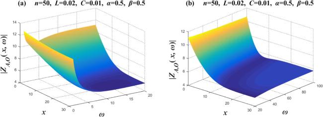
Figure 3. Set n = 50 and $\alpha =\beta =\mathrm{0.5.}$ Two 3D amplitude-frequency characteristic curves of the equivalent complex impedance ZA,O(x, ω), where figures (a) and (b) are two segmented function images, respectively. |
Case 2. Amplitude-frequency characteristic image when α = 0.5, β = 1.0
Figure 4 takes the value of n = 50, $L=0.02,$ $C=0.01,$ $\alpha =0.5$ and $\beta =1,$ and divides the ω segment into $\omega =1\sim 20$ and $\omega =20\sim 100$ for drawing. Take $x=0\to 30$ in the image; specifically, the 3D image drawn represents the amplitude-frequency characteristics of 31 complex impedances. Figure 4(a) shows that $\left|{Z}_{AO}(x,\omega )\right|$ changes significantly when $\omega =1\sim 5,$ and its corresponding $\left|{Z}_{AO}(x,\omega )\right|$ decreases as ω increases. Figure 4(b) shows that when $\omega \geqslant 20$ increases with ω, its corresponding $\left|{Z}_{AO}(x,\omega )\right|$ also increases. Then, we observe the law of change between $\left|{Z}_{AO}(x,\omega )\right|$ and x. Figure 4(a) shows that $\left|{Z}_{AO}(x,\omega )\right|$ hardly changes as x increases when $\omega =1.$ When $\omega =10$ is present, $\left|{Z}_{AO}(x,\omega )\right|$ decreases as x increases. Figure 4(b) shows that when $\omega \gt 20,$ for a definite ω value, between $x=15\to 30,$ its corresponding $\left|{Z}_{AO}(x,\omega )\right|$ does not change significantly with the change in x. And its corresponding $\left|{Z}_{AO}(x,\omega )\right|$ decreases significantly with the increase in x between $x=0\to 10.$
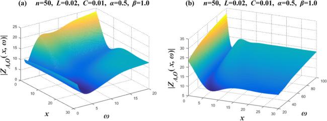
Figure 4. Set n = 50, $\alpha =0.5$ and $\beta =1.$ Two 3D amplitude-frequency characteristic curves of the equivalent complex impedance ZA,O(x, ω), where figures (a) and (b) are two segmented function images, respectively. |
Case 3. Amplitude-frequency characteristic image when α = 1.0, β = 0.5
Figure 5 takes the value of n = 50, $L=0.02,$ $C=0.01,$ $\alpha =1$ and $\beta =0.5,$ and we divide ω into $\omega =1\sim 20$ and $\omega =20\sim 100$ for drawing. Take $x=0\to 30$ in the image; the 3D image drawn represents the amplitude-frequency characteristics of 31 complex impedances. The changes in figure 5(a) are relatively difficult to describe and are only suitable for understanding by looking at the image. Of course, for each determined x value, it can be described. Figure 5(b) shows that when $\omega \geqslant 20$ increases with ω, its corresponding $\left|{Z}_{AO}(x,\omega )\right|$ decreases. Then, we observe the law of change between $\left|{Z}_{AO}(x,\omega )\right|$ and x. Figure 5(b) shows that when $\omega \gt 20,$ for a definite ω value, between $x=15\to 30,$ its corresponding $\left|{Z}_{AO}(x,\omega )\right|$ does not change significantly with the change in x. And its corresponding $\left|{Z}_{AO}(x,\omega )\right|$ decreases significantly with the increase in x between $x=0\to 10.$
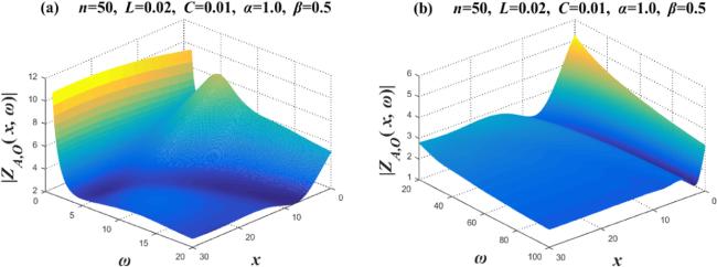
Figure 5. Set n = 50, $\alpha =1$ and $\beta =\mathrm{0.5.}$ Two 3D amplitude-frequency characteristic curves of the equivalent complex impedance ZA,O(x, ω), where figures (a) and (b) are two segmented function images, respectively. |
Case 4. Amplitude-frequency characteristic image when α = 0.0, β = 1.0
When $\alpha =0.0,\beta =1.0,$ equation (2 ) degenerates to ${Z}_{L}=j\omega L,$ ${Z}_{C}=1/C.$ This is equivalent to ${Z}_{L}=j\omega L$ being a pure inductor, and ${Z}_{C}=1/C=R$ being a pure resistor. Specifically, the circuit network at $\alpha =0.0,\beta =1.0$ is actually equivalent to the circuit network composed of RL, and its characteristics are shown in figure 6. Segment ω into $\omega =1\sim 20$ and $\omega =20\sim 100$ for drawing. Take $x=0\to 30$ in the image; the 3D image drawn represents the amplitude-frequency characteristics of 31 complex impedances. Figure 6(a) shows that $\left|{Z}_{AO}(x,\omega )\right|$ increases as ω increases. Figure 6(b) shows that when $\omega \geqslant 20$ increases with ω, its corresponding $\left|{Z}_{AO}(x,\omega )\right|$ also increases. Then, we observe the law of change between $\left|{Z}_{AO}(x,\omega )\right|$ and x. Figure 6(a) shows that $\left|{Z}_{AO}(x,\omega )\right|$ hardly changes as x increases when $\omega =1.$ When $\omega \geqslant 10,$ $\left|{Z}_{AO}(x,\omega )\right|$ decreases as x increases. Figure 6(b) shows that when $\omega \gt 20,$ for a definite ω value, between $x=15\to 30,$ its corresponding $\left|{Z}_{AO}(x,\omega )\right|$ does not change significantly with the change in x. And its corresponding $\left|{Z}_{AO}(x,\omega )\right|$ decreases significantly with the increase in x between $x=0\to 10.$
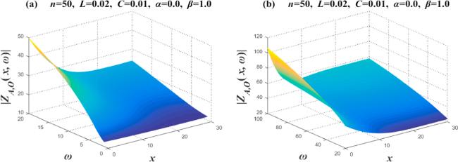
Figure 6. Set n = 50, $\alpha =0$ and $\beta =1.$ Two 3D amplitude-frequency characteristic curves of the equivalent complex impedance ZA,O(x, ω), where figures (a) and (b) are two segmented function images, respectively. |
Case 5. Amplitude-frequency characteristic image when α = 1.0, β = 0
When $\alpha =1.0,\beta =0.0,$ equation (2 ) degenerates to ${Z}_{L}=L,$ ${Z}_{C}=\text{\unicode{x02212}}j/\omega C.$ This is equivalent to ${Z}_{L}=L$ being a pure resistor and ${Z}_{C}=-1/j\omega C$ being a pure capacitor. Specifically, the circuit network at $\alpha =1.0,\beta =0.0$ is actually equivalent to the circuit network composed of RC, and its characteristics are shown in figure 7. Figure 7(a) shows that $\left|{Z}_{AO}(x,\omega )\right|$ increases as ω increases. Figure 7(b) shows that when $\omega \geqslant 20$ increases with ω, its corresponding $\left|{Z}_{AO}(x,\omega )\right|$ decreases. Then, we observe the law of change between $\left|{Z}_{AO}(x,\omega )\right|$ and x. Figure 7(a) shows that $\left|{Z}_{AO}(x,\omega )\right|$ does not change significantly with the change in x. Figure 7(b) shows that when $\omega \geqslant 20,$ $x\leqslant 10,$ for a definite ω value, $\left|{Z}_{AO}(x,\omega )\right|$ decreases significantly with the increase in x, and $\left|{Z}_{AO}(x,\omega )\right|$ does not change significantly with the change in x between $x=20\to 30.$
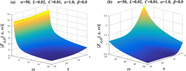
Figure 7. Set n = 50, $\alpha =1$ and $\beta =0.$ Two 3D amplitude-frequency characteristic curves of the equivalent complex impedance ZA,O(x, ω), where figures (a) and (b) are two segmented function images, respectively. |
Case 6. Amplitude-frequency characteristic image when α = 1.0, β = 1.0
When $\alpha =1.0,\beta =1.0,$ equation (2 ) degenerates to ${Z}_{L}=j\omega L,$ ${Z}_{C}=-j/\omega C,$ which is equivalent to an integer-order LC circuit network consisting of pure inductors and pure capacitors, and its characteristics are shown in figure 8. Segment ω into $\omega =1\sim 20$ and $\omega =20\sim 100$ for drawing. Take $x=0\to 30$ in the images; the 3D image drawn represents the amplitude-frequency characteristics of 31 complex impedances. The images show the phenomenon of partial regular oscillation and partial irregular oscillation for $\left|{Z}_{AO}(x,\omega )\right|.$
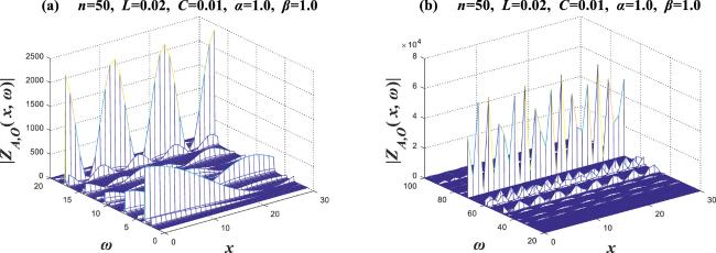
Figure 8. Set n = 50 and $\alpha =\beta =1.$ Two 3D amplitude-frequency characteristic curves of the equivalent complex impedance ZA,O(x, ω), where figures (a) and (b) are two segmented function images, respectively. |
4.2. Visualized phase-frequency characteristics
Case 1. Images of phase-frequency characteristics when α = β = 0.5
To clearly show the phase-frequency characteristic image at $\alpha =\beta =0.5,$ we consider the significant difference in variation at $\omega =1\unicode{x0007E}10,$ and we will plot $\omega =1\sim 100$ into $\omega =1\sim 20$ and $\omega =20\sim 100.$ In the phase angle $Arg[{Z}_{AO}(x,\omega )]$ of the complex impedance, x is the coordinate of any point on the horizontal axis A0An, and ω is the circular frequency of the alternating current of the input circuit.
Figure 9 takes the values of n = 50, $L=0.02,$ $C=0.01,$ $\alpha =\beta =0.5,$ and we segment ω into $\omega =1\sim 20$ and $\omega =20\sim 100$ for drawing. Take $x=0\to 30$ in the image; the 3D image drawn represents the phase-frequency characteristics of 31 complex impedances. Figure 9(a) shows that $\phi [{Z}_{AO}(x,\omega )]$ changes significantly; its corresponding $\phi [{Z}_{AO}(x,\omega )]$ increases as ω increases when $x=0\to 10.$ Figure 9(b) shows that when $\omega \geqslant 20$ increases with ω, its corresponding $\phi \left|{Z}_{AO}(x,\omega )\right|$ does not change significantly. When $20\leqslant \omega \leqslant 100$ and $0\leqslant x\leqslant 20,$ the $\phi [{Z}_{AO}(x,\omega )]$ decreases first and then increases as x increases, which is like a sink, and there seems to be a platform on the right side when x>20.
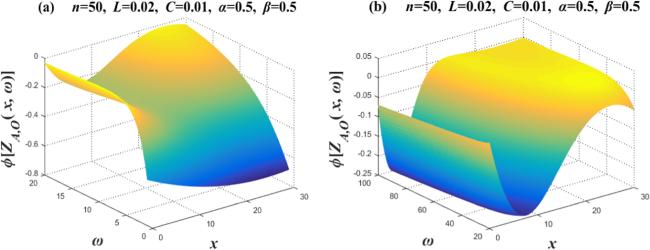
Figure 9. Set n = 50, $\alpha =\beta =\mathrm{0.5.}$ Two 3D phase-frequency characteristic curves of the equivalent complex impedance ZA,O(x, ω), where figures (a) and (b) are two segmented function images, respectively. |
Case 2. Images of phase-frequency characteristics when α = 0.5, β = 1.0
Figure 10 takes the values of n = 50, $L=0.02,$ $C=0.01,$ $\alpha =0.5$ and $\beta =1,$ and we segment ω into $\omega =1\sim 20$ and $\omega =20\sim 100$ for drawing. Take $x=0\to 30$ in the image; clearly, the 3D image drawn represents the amplitude-frequency characteristics of 31 complex impedances. Figure 10(a) shows that $\phi [{Z}_{AO}(x,\omega )]$ changes significantly when $\omega =1\sim 5;$ its corresponding $\phi [{Z}_{AO}(x,\omega )]$ increases as ω increases. In figure 10(b), there are significantly different variation patterns in different regions of $0\leqslant x\leqslant 10$ and $x\gt 20.$ There is a groove between $0\leqslant x\leqslant 10,$ and there seems to be a platform in the area of $x\gt 20.$
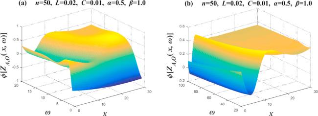
Figure 10. Set n = 50, $\alpha =0.5$ and $\beta =\mathrm{1.0.}$ Two 3D phase-frequency characteristic curves of the equivalent complex impedance ZA,O(x, ω), where figures (a) and (b) are two segmented function images, respectively. |
Case 3. Images of phase-frequency characteristics when α = 1.0, β = 0.5
Figure 11 takes the values of n = 50, $L=0.02,$ $C=0.01,$ $\alpha =1$ and $\beta =0.5.$ Image 11 and Image 10 seem to have some similarities, but their spirit is different. When you compare their vertical coordinates, you will find that the vertical coordinates of figure 10(a) are −1.0∼1.0, while the vertical coordinates of figure 11(a) are −2.0∼0.0; the vertical coordinates of figure 10(b) are −0.2∼0.6, while the vertical coordinates of figure 11(b) are −1.0∼−0.2. Specifically, their images seem to have a translational relationship.
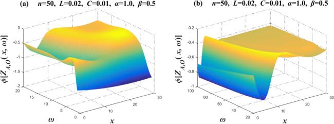
Figure 11. Set n = 50, $\alpha =1$ and $\beta =\mathrm{0.5.}$ Two 3D phase-frequency characteristic curves of the equivalent complex impedance ZA,O(x, ω), where figures (a) and (b) are two segmented function images, respectively. |
Case 4. Images of phase-frequency characteristics when α = 0, β = 1.0
When $\alpha =0.0,\beta =1.0,$ equation (2 ) degenerates to ${Z}_{L}=j\omega L,$ ${Z}_{C}=1/C.$ This is equivalent to ${Z}_{L}=j\omega L$ being a pure inductor and ${Z}_{C}=1/C=R$ being equivalent to a pure resistor. Image 12 and Image 9 seem to have some similarities, but their spirit is different. When you compare their vertical coordinates, you will find that the vertical coordinates of figure 9(a) are −0.8∼0.0, while the vertical coordinates of figure 12(a) are 0.0∼0.8; the vertical coordinates of figure 9(b) are -0.25∼0.05, while the vertical coordinates of figure 12(b) are 0.5∼0.8. Specifically, their images seem to have a translational relationship relative to the vertical axis.
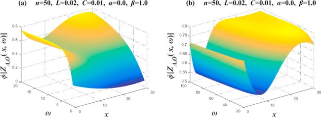
Figure 12. Set n = 50, $\alpha =0.0$ and $\beta =\mathrm{1.0.}$ Two 3D phase-frequency characteristic curves of the equivalent complex impedance ZA,O(x, ω), where figures (a) and (b) are two segmented function images, respectively. |
Case 5. Images of phase-frequency characteristics when α = 1, β = 0
When $\alpha =0.0,\beta =1.0,$ then equation (2 ) degenerates to ${Z}_{L}=j\omega L,$ ${Z}_{C}=1/C.$ This is equivalent to ${Z}_{L}=j\omega L$ being a pure inductor and ${Z}_{C}=1/C=R$ being equivalent to a pure resistor. Image 13 and Image 12 seem to have some similarities, but their spirit is different. When you compare their vertical coordinates, you will find that the vertical coordinates of figure 12(a) are 0.0 ∼ 0.8, while the vertical coordinates of figure 13(a) are −1.6 ∼ −0.8; the vertical coordinates of figure 12(b) are 0.5 ∼ 0.8, while the vertical coordinates of figure 13(b) are −1.05 ∼ −0.75. Specifically, their images seem to have a translational relationship relative to the vertical axis.
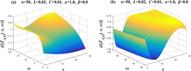
Figure 13. Set n = 50, $\alpha =1$ and $\beta =0.$ Two 3D phase-frequency characteristic curves of the equivalent complex impedance ZA,O(x, ω), where figures (a) and (b) are two segmented function images, respectively. |
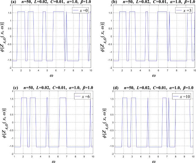
Case 6. Images of phase-frequency characteristics when α = β = 1.0
Figure 14 takes the values of $n=50,$ $L=0.02,$ $C=0.01,$ $\alpha =\beta =1.0,$ giving four 2D phase-frequency characteristic curves of the equivalent complex impedance ${Z}_{AO}(x,\omega ),$ where x = {0, 3, 6, 10} represents the complex impedance at four positions.
Figure 14. Set n = 50, $\alpha =1$ and $\beta =1.$ Four 2D phase-frequency characteristic curves of the equivalent complex impedance ZA,O(x, ω), where figures (a), (b), (c), and (d) show the phase-frequency function images of the four node positions x = {0, 3, 6, 10}, respectively. |
The phase $\phi [{Z}_{AO}(x,\omega )]$ follows a series of jumping states with the change in frequency, as if it is an irregular pulse. We can clearly see its changing characteristics from the four images. We can see $\phi \in [-\pi /2,\,\pi /2]$, which is an irregular change.
5. Conclusion and comment
This article derives three general impedance formulae of the FO 3 × n Fan network model. We analyze the influence of some variables on the amplitude-frequency and phase-frequency characteristics in three different cases. At the same time, via the analysis of the FOC 3 × n Fan network, new impedance and phase results are derived. In addition, we use Matlab to draw a graphical model to describe the influence of several variables on amplitude-frequency and phase-frequency characteristics. From the series images of the amplitude-frequency and phase-frequency characteristics, problems under various conditions are considered and studied, such as RCα circuits, RLβ circuits, LβCα circuits and LC circuits.
Acknowledgments
This work is supported by the National Training Programs of Innovation and Entrepreneurship for Undergraduates (Grant No. 202210304006Z).
Declaration of competing interest
The authors declare that they have no known competing financial interests or personal relationships that could have appeared to influence the work reported in this paper.