


1. Introduction
The nonlinear Schrödinger (NLS) equation,
$\begin{eqnarray}{\rm{i}}{q}_{t}-{q}_{{xx}}-2\epsilon | q{| }^{2}q=0,\end{eqnarray}$
as one of the most famous integrable systems, is known as a ‘universal’ model [1], which means it appears as a governing model in various physical phenomena. Here ‘i’ is the imaginary unit, ε = ± 1, ∣q∣2 = qq* and * stands for complex conjugate. It emerges in describing wave packages in deep water [2, 3], plasma physics [4], optical fiber [5, 6], etc. In addition, the NLS equation with various external potentials (known also as the Gross–Pitaevskii (GP) equation [7–9]) is also the governing model in nonlinear optics and Bose–Einstein condensates (BEC) [10]. One can refer to [11] for more references and applications of the NLS equation and its extensions.The NLS equation with x-coefficient can describe nonlinear waves in non-uniformity media [12–15]. Such equations have been shown to be integrable in the sense of having Lax pairs, with the spectral parameter η satisfying ηt ≠ 0, which are referred to non-isospectral nonlinear Schrödinger equations (NNLSEs). In this paper, we will investigate the following three NNLSEs:1.1a ) via gauge transformations, e.g. [16], they are physically useful in BEC: the NNLSE-I is the GP equation with a linear potential [17], while the NNLSE-II can provide solutions to the GP equation with a parabolic potential and a gain term e.g. [18]. The NNLSE-III can provide space-time localized soliton waves on zero background [16, 19]. So far, integrable methods, such as the inverse scattering transform [12–14] and bilinear method [16], have been applied to obtain explicit solutions of the above equations. Yet in this paper, we construct their solutions by means of a completely direct method, namely, the Cauchy matrix approach.
$\begin{eqnarray}{\rm{i}}{q}_{1,t}-{q}_{1,{xx}}-2| {q}_{1}{| }^{2}{q}_{1}+2\alpha {{xq}}_{1}=0,\end{eqnarray}$
$\begin{eqnarray}{\rm{i}}{q}_{2,t}-{q}_{2,{xx}}-2| {q}_{2}{| }^{2}{q}_{2}+{\rm{i}}\beta {\,({{xq}}_{2})}_{x}=0,\end{eqnarray}$
$\begin{eqnarray}{\rm{i}}{q}_{3,t}-x\,({q}_{3,{xx}}+2| {q}_{3}{| }^{2}{q}_{3})-2{q}_{3,x}-2{q}_{3}\,{\partial }^{-1}| {q}_{3}{| }^{2}=0,\end{eqnarray}$
where α and β are real constants, and ∂−1 stands for the integration operator with respect to x. We denote these equations NNLSE-I, NNLSE-II, and NNLSE-III for short, respectively. They correspond to time-dependant spectral parameter η with time evolutions ηt = α, ηt = − iβη and ηt = −2η2, respectively, where $\alpha ,\beta \in {\mathbb{R}}$, e.g. [16]. Although the NNLSE-I and NNLSE-II can be converted to the NLS equation (The Cauchy matrix approach is a method to construct and study integrable equations by means of the Sylvester-type equations. It is first systematically introduced in [20] to investigate integrable quadrilateral equations and later developed in [21, 22] to more general cases. It has also been applied to the Zakharov–Shabat–Ablowitz–Kaup–Newell–Segur (ZS-AKNS) system [23], equations with self-consistent sources [24], and the self-dual Yang-Mills equation [25, 26], etc. The purpose of this paper is not only to construct solutions to the three NNLSEs in (1.2 ), but also to extend the Cauchy matrix approach to the non-isospectral case, as the Sylvester-type equation in the Cauchy matrix scheme of the ZS-AKNS system is a typical type (see [22, 27] for the Korteweg–de Vries (KdV) and Kadomtsev–Petviashvili (KP) type equations). One will see that the non-isospectral extension of the Cauchy matrix scheme is quite non-trivial compared with the isospectral case [23].
This paper is organized as follows. Our plan is in the first step to derive three unreduced non-isospectral Schrödinger systems using the Cauchy matrix approach. This will be described in section 2 . Then in section 3 , we present solution formulae of these unreduced systems. These formulae guide us to implement reduction so that solutions of the NNLSEs are obtained, which will be done in section 4 . Dynamics of these solutions are illustrated also in this section. Finally, conclusions are given in section 5 . There is an appendix section where solutions of the Sylvester equation with lower triangular Toeplitz matrices are presented.
2. Cauchy matrix approach to unreduced NNLSEs
In this section, we describe the Cauchy matrix approach for unreduced NNLSEs.
2.1. Sylvester equation and master functions
We start from the Sylvester equation of the following type (see [23, 25]):2.1 ) is given by
$\begin{eqnarray}{\boldsymbol{K}}{\boldsymbol{M}}-{\boldsymbol{M}}{\boldsymbol{K}}={\boldsymbol{r}}{{\boldsymbol{s}}}^{{\rm{T}}},\end{eqnarray}$
in which the involved elements are block matrices in the form of $\begin{eqnarray}\begin{array}{l}{\boldsymbol{K}}=\left(\begin{array}{cc}{{\boldsymbol{K}}}_{1} & 0\\ 0 & {{\boldsymbol{K}}}_{2}\end{array}\right),\,{\boldsymbol{M}}=\left(\begin{array}{cc}0 & {{\boldsymbol{M}}}_{1}\\ {{\boldsymbol{M}}}_{2} & 0\end{array}\right),\\ {\boldsymbol{r}}=\left(\begin{array}{cc}{{\boldsymbol{r}}}_{1} & 0\\ 0 & {{\boldsymbol{r}}}_{2}\end{array}\right),\,{\boldsymbol{s}}=\left(\begin{array}{cc}0 & {{\boldsymbol{s}}}_{1}\\ {{\boldsymbol{s}}}_{2} & 0\end{array}\right),\end{array}\end{eqnarray}$
where ${{\boldsymbol{K}}}_{i}\in {{\mathbb{C}}}_{N\times N}\,[t],{{\boldsymbol{M}}}_{i}\in {{\mathbb{C}}}_{N\times N}\,[x,t],{{\boldsymbol{r}}}_{i},{{\boldsymbol{s}}}_{i}\in {{\mathbb{C}}}_{N\times 1}\,[x,t]$, for i = 1, 2. An equivalent form of ( $\begin{eqnarray}{{\boldsymbol{K}}}_{1}\,{{\boldsymbol{M}}}_{1}\,-\,{{\boldsymbol{M}}}_{1}\,{{\boldsymbol{K}}}_{2}\,=\,{{\boldsymbol{r}}}_{1}\,{{\boldsymbol{s}}}_{2}^{{\rm{T}}},\end{eqnarray}$
$\begin{eqnarray}{{\boldsymbol{K}}}_{2}\,{{\boldsymbol{M}}}_{2}\,-\,{{\boldsymbol{M}}}_{2}\,{{\boldsymbol{K}}}_{1}\,=\,{{\boldsymbol{r}}}_{2}\,{{\boldsymbol{s}}}_{1}^{{\rm{T}}}.\end{eqnarray}$
We assume matrices K1 and K2 do not share any eigenvalues, so that the Sylvester equation (2.1 ) has a unique solution M for given K, r, s [28]. By these elements we define master functions
$\begin{eqnarray}{{\boldsymbol{S}}}^{(i,j\,)\,}\doteq {{\boldsymbol{s}}}^{{\rm{T}}}{{\boldsymbol{K}}}^{j}{\left(\,,{{\boldsymbol{I}}}_{2N}+{\boldsymbol{M}}\right)}^{-1}{{\boldsymbol{K}}}^{i}{\boldsymbol{r}}=\left(\begin{array}{cc}{s}_{1}^{(i,j\,)} & {s}_{2}^{(i,j\,)}\\ {s}_{3}^{(i,j\,)} & {s}_{4}^{(i,j\,)}\end{array}\right),\,\,\,\,(i,j\in {\mathbb{Z}}),\end{eqnarray}$
where I2N is the 2N th-order unit matrix and of which the more explicit versions are $\begin{eqnarray}{s}_{1}^{(i,j\,)}=-{{\boldsymbol{s}}}_{2}^{{\rm{T}}}\,{{\boldsymbol{K}}}_{2}^{j}{\left(\,,{{\boldsymbol{I}}}_{N}-{{\boldsymbol{M}}}_{2}\,{{\boldsymbol{M}}}_{1}\right)}^{-1}{{\boldsymbol{M}}}_{2}\,{{\boldsymbol{K}}}_{1}^{i}\,{{\boldsymbol{r}}}_{1},\end{eqnarray}$
$\begin{eqnarray}{s}_{2}^{(i,j\,)}={{\boldsymbol{s}}}_{2}^{{\rm{T}}}\,{{\boldsymbol{K}}}_{2}^{j}{\left(\,,{{\boldsymbol{I}}}_{N}-{{\boldsymbol{M}}}_{2}\,{{\boldsymbol{M}}}_{1}\right)}^{-1}{{\boldsymbol{K}}}_{2}^{i}\,{{\boldsymbol{r}}}_{2},\end{eqnarray}$
$\begin{eqnarray}{s}_{3}^{(i,j\,)}={{\boldsymbol{s}}}_{1}^{{\rm{T}}}\,{{\boldsymbol{K}}}_{1}^{j}{\left(\,,{{\boldsymbol{I}}}_{N}-{{\boldsymbol{M}}}_{1}\,{{\boldsymbol{M}}}_{2}\right)}^{-1}{{\boldsymbol{K}}}_{1}^{i}\,{{\boldsymbol{r}}}_{1},\end{eqnarray}$
$\begin{eqnarray}{s}_{4}^{(i,j\,)}=-{{\boldsymbol{s}}}_{1}^{{\rm{T}}}\,{{\boldsymbol{K}}}_{1}^{j}{\left(\,,{{\boldsymbol{I}}}_{N}-{{\boldsymbol{M}}}_{1}\,{{\boldsymbol{M}}}_{2}\right)}^{-1}{{\boldsymbol{M}}}_{1}\,{{\boldsymbol{K}}}_{2}^{i}\,{{\boldsymbol{r}}}_{2}.\end{eqnarray}$
In addition, a difference-product formula can be formulated from (2.1 ) as
$\begin{eqnarray}{{\boldsymbol{S}}}^{(i+1,j\,)}-{{\boldsymbol{S}}}^{(i,j+1)}={{\boldsymbol{S}}}^{(0,j\,)\,}{{\boldsymbol{S}}}^{(i,0)}.\end{eqnarray}$
2.2. Unreduced NNLSE-I
To derive an unreduced form of the NNLSE-I equation, let us introduce dispersion relations of r and s as follows,2.1 ), which gives rise to2.7b ) and (2.9 ) into it yields2.12 ) yields2.7b ), (2.9 ) and (2.10 ) into (2.15 ), and then left-multiplied by ${\left({{\boldsymbol{I}}}_{2N}+{\boldsymbol{M}}\right)}^{-1}$, we get2.13 ), it is easy to get x-derivative of S(i,j), which reads [23]2.13 ) we have2.7b ), (2.9 ) and (2.16 ) into (2.18 ), we have2.17 ) and get second-order derivatives of S(i,j) with respect to x, which which reads
$\begin{eqnarray}{{\boldsymbol{r}}}_{x}=\displaystyle \frac{1}{2}{\boldsymbol{K}}{\boldsymbol{r}}{\boldsymbol{a}},\quad {{\boldsymbol{s}}}_{x}=-\displaystyle \frac{1}{2}{{\boldsymbol{K}}}^{{\rm{T}}}{\boldsymbol{s}}{\boldsymbol{a}},\end{eqnarray}$
$\begin{eqnarray}{{\boldsymbol{r}}}_{t}=\left(-\displaystyle \frac{1}{2}{{\boldsymbol{K}}}^{2}+\alpha x\right)\,{\boldsymbol{r}}{\boldsymbol{a}},\quad {{\boldsymbol{s}}}_{t}=\left(\displaystyle \frac{1}{2}{\left(\,,{{\boldsymbol{K}}}^{{\rm{T}}}\right)}^{2}-\alpha x\right)\,{\boldsymbol{s}}{\boldsymbol{a}},\end{eqnarray}$
where $\begin{eqnarray}{\boldsymbol{a}}=\left(\begin{array}{cc}1 & 0\\ 0 & -1\end{array}\right)\end{eqnarray}$
and matrix K obeys the evolution $\begin{eqnarray}{{\boldsymbol{K}}}_{t}=\displaystyle \frac{{\rm{d}}}{{\rm{d}}t}{\boldsymbol{K}}\,(t)=2\alpha ,\,\,\alpha \in {\mathbb{R}}.\end{eqnarray}$
In addition, we assume Kt and K commute. Then one can derive the evolution of M by taking a derivative of the Sylvester equation ( $\begin{eqnarray*}{{\boldsymbol{K}}}_{t}\,{\boldsymbol{M}}+{\boldsymbol{K}}{{\boldsymbol{M}}}_{t}-{{\boldsymbol{M}}}_{t}\,{\boldsymbol{K}}-{\boldsymbol{M}}{{\boldsymbol{K}}}_{t}={{\boldsymbol{r}}}_{t}\,{{\boldsymbol{s}}}^{{\rm{T}}}+{\boldsymbol{r}}{{\boldsymbol{s}}}_{t}^{{\rm{T}}}.\end{eqnarray*}$
Substituting ( $\begin{eqnarray*}{\boldsymbol{K}}{{\boldsymbol{M}}}_{t}-{{\boldsymbol{M}}}_{t}\,{\boldsymbol{K}}=\displaystyle \frac{1}{2}\,(-{{\boldsymbol{K}}}^{2}{\boldsymbol{r}}{\boldsymbol{a}}{{\boldsymbol{s}}}^{{\rm{T}}}+{\boldsymbol{r}}{\boldsymbol{a}}{{\boldsymbol{s}}}^{{\rm{T}}}{{\boldsymbol{K}}}^{2}),\end{eqnarray*}$
which leads us to a Sylvester equation, $\begin{eqnarray*}{\boldsymbol{K}}\,\left({{\boldsymbol{M}}}_{t}+\displaystyle \frac{1}{2}\,({\boldsymbol{K}}{\boldsymbol{r}}{\boldsymbol{a}}{{\boldsymbol{s}}}^{{\rm{T}}}+{\boldsymbol{r}}{\boldsymbol{a}}{{\boldsymbol{s}}}^{{\rm{T}}}{\boldsymbol{K}})\,\right)-\left({{\boldsymbol{M}}}_{t}+\displaystyle \frac{1}{2}\,({\boldsymbol{K}}{\boldsymbol{r}}{\boldsymbol{a}}{{\boldsymbol{s}}}^{{\rm{T}}}+{\boldsymbol{r}}{\boldsymbol{a}}{{\boldsymbol{s}}}^{{\rm{T}}}{\boldsymbol{K}})\,\right)\,{\boldsymbol{K}}=0.\end{eqnarray*}$
It has a unique zero solution in the light of assumption that K1 and K2 do not share any eigenvalues. Thus we have $\begin{eqnarray}{{\boldsymbol{M}}}_{t}=-\displaystyle \frac{1}{2}\,({\boldsymbol{K}}{\boldsymbol{r}}{\boldsymbol{a}}{{\boldsymbol{s}}}^{{\rm{T}}}+{\boldsymbol{r}}{\boldsymbol{a}}{{\boldsymbol{s}}}^{{\rm{T}}}{\boldsymbol{K}}).\end{eqnarray}$
One can also find [23] $\begin{eqnarray}{{\boldsymbol{M}}}_{x}=\displaystyle \frac{1}{2}{\boldsymbol{r}}{\boldsymbol{a}}{{\boldsymbol{s}}}^{{\rm{T}}}.\end{eqnarray}$
Next we are going to derive the derivative of S(i,j). Let us define the auxiliary vector, $\begin{eqnarray}{{\boldsymbol{u}}}^{(i)}={\left({{\boldsymbol{I}}}_{2N}+{\boldsymbol{M}}\right)}^{-1}{{\boldsymbol{K}}}^{i}{\boldsymbol{r}},\end{eqnarray}$
which is connected with S(i,j) by $\begin{eqnarray}{{\boldsymbol{S}}}^{(i,j\,)}={{\boldsymbol{s}}}^{{\rm{T}}}{{\boldsymbol{K}}}^{j}{{\boldsymbol{u}}}^{(i)}.\end{eqnarray}$
The derivative of u(i) with respect to x reads [23] $\begin{eqnarray}{{\boldsymbol{u}}}_{x}^{(i)}=\displaystyle \frac{1}{2}\left(\,,{{\boldsymbol{u}}}^{(i+1)\,}a-{{\boldsymbol{u}}}^{(0)\,}a{{\boldsymbol{S}}}^{(i,0)}\right).\end{eqnarray}$
To derive the derivative of u(i) with respect to t, taking t-derivative in ( $\begin{eqnarray}{{\boldsymbol{M}}}_{t}\,{{\boldsymbol{u}}}^{(i)}+({{\boldsymbol{I}}}_{2N}+{\boldsymbol{M}})\,{{\boldsymbol{u}}}_{t}^{(i)}=i{{\boldsymbol{K}}}^{i-1}{{\boldsymbol{K}}}_{t}\,{\boldsymbol{r}}+{{\boldsymbol{K}}}^{i}{{\boldsymbol{r}}}_{t},\end{eqnarray}$
and we substitute( $\begin{eqnarray}{{\boldsymbol{u}}}_{t}^{(i)}=\displaystyle \frac{1}{2}\left(\,,4i\alpha {{\boldsymbol{u}}}^{(i-1)}-{{\boldsymbol{u}}}^{(i+2)\,}{\boldsymbol{a}}+{{\boldsymbol{u}}}^{(1)\,}{\boldsymbol{a}}{{\boldsymbol{S}}}^{(i,0)}+{{\boldsymbol{u}}}^{(0)\,}{\boldsymbol{a}}{{\boldsymbol{S}}}^{(i,1)}\right)+\alpha x{{\boldsymbol{u}}}^{(i)\,}{\boldsymbol{a}}.\end{eqnarray}$
Using the relation ( $\begin{eqnarray}{{\boldsymbol{S}}}_{x}^{(i,j\,)}=\displaystyle \frac{1}{2}\left(\,,{{\boldsymbol{S}}}^{(i+1,j\,)\,}{\boldsymbol{a}}-{\boldsymbol{a}}{{\boldsymbol{S}}}^{(i,j+1)}-{{\boldsymbol{S}}}^{(0,j\,)\,}{\boldsymbol{a}}{{\boldsymbol{S}}}^{(i,0)}\right).\end{eqnarray}$
For the t-derivative of S(i,j), from ( $\begin{eqnarray}{{\boldsymbol{S}}}_{t}^{(i,j\,)}={{\boldsymbol{s}}}_{t}^{{\rm{T}}}\,{{\boldsymbol{K}}}^{j}{{\boldsymbol{u}}}^{(i)}+j{{\boldsymbol{s}}}^{{\rm{T}}}{{\boldsymbol{K}}}^{j-1}{{\boldsymbol{K}}}_{t}\,{{\boldsymbol{u}}}^{(i)}+{{\boldsymbol{s}}}^{{\rm{T}}}{{\boldsymbol{K}}}^{j}{{\boldsymbol{u}}}_{t}^{(i)}.\end{eqnarray}$
Then, substituting ( $\begin{eqnarray}\begin{array}{l}{{\boldsymbol{S}}}_{t}^{(i,j\,)}=\displaystyle \frac{1}{2}\left(\,,{\boldsymbol{a}}{{\boldsymbol{S}}}^{(i,j+2)}-{{\boldsymbol{S}}}^{(i+2,j\,)\,}{\boldsymbol{a}}+{{\boldsymbol{S}}}^{(1,j\,)\,}{\boldsymbol{a}}{{\boldsymbol{S}}}^{(i,0)}+{{\boldsymbol{S}}}^{(0,j\,)\,}{\boldsymbol{a}}{{\boldsymbol{S}}}^{(i,1)}\right)\\ +\alpha \left(\,,x\,({{\boldsymbol{S}}}^{(i,j\,)\,}{\boldsymbol{a}}-{\boldsymbol{a}}{{\boldsymbol{S}}}^{(i,j\,)})+2\,(\,j{{\boldsymbol{S}}}^{(i,j-1)}+i{{\boldsymbol{S}}}^{(i-1,j\,)})\right).\end{array}\end{eqnarray}$
One can repeatedly use ( $\begin{eqnarray}\begin{array}{l}{{\boldsymbol{S}}}_{{xx}}^{(i,j\,)}=\displaystyle \frac{1}{4}\,({{\boldsymbol{S}}}^{(i,j+2)}+{{\boldsymbol{S}}}^{(i+2,j\,)}-2{\boldsymbol{a}}{{\boldsymbol{S}}}^{(i+1,j+1)\,}{\boldsymbol{a}}\\ +2{\boldsymbol{a}}{{\boldsymbol{S}}}^{(0,j+1)\,}{\boldsymbol{a}}{{\boldsymbol{S}}}^{(i,0)}-2{{\boldsymbol{S}}}^{(0,j\,)\,}{\boldsymbol{a}}{{\boldsymbol{S}}}^{(i+\mathrm{1,0})\,}{\boldsymbol{a}}\\ -{{\boldsymbol{S}}}^{(1,j\,)\,}{{\boldsymbol{S}}}^{(i,0)}+{{\boldsymbol{S}}}^{(0,j\,)\,}{{\boldsymbol{S}}}^{(i,1)}\\ +2{{\boldsymbol{S}}}^{(0,j\,)\,}{\boldsymbol{a}}{{\boldsymbol{S}}}^{(\mathrm{0,0})\,}{\boldsymbol{a}}{{\boldsymbol{S}}}^{(i,0)}).\end{array}\end{eqnarray}$
Next, let us define2.17 ) and (2.19 ):2.6 ), we obtain the following relations by choosing (i, j) = (0, 1), (1, 0), (0, 0), respectively:2.21 ) we obtain a closed system of u2 and u3 as the unreduced form of the NNLSE-I:
$\begin{eqnarray}{\boldsymbol{U}}\doteq {{\boldsymbol{S}}}^{(\mathrm{0,0})},\,\,\,{u}_{i}={s}_{i}^{(0,0)},\,\,(i=1,2,3,4),\end{eqnarray}$
one has the following by taking i = j = 0 in ( $\begin{eqnarray*}\begin{array}{l}{{\boldsymbol{U}}}_{x}=\displaystyle \frac{1}{2}\,({{\boldsymbol{S}}}^{(\mathrm{1,0})\,}{\boldsymbol{a}}-{\boldsymbol{a}}{{\boldsymbol{S}}}^{(\mathrm{0,1})}-{\boldsymbol{U}}{\boldsymbol{a}}{\boldsymbol{U}}),\\ {{\boldsymbol{U}}}_{{xx}}=\displaystyle \frac{1}{4}\,({{\boldsymbol{S}}}^{(\mathrm{2,0})}+{{\boldsymbol{S}}}^{(\mathrm{0,2})}-2{\boldsymbol{a}}{{\boldsymbol{S}}}^{(\mathrm{1,1})\,}{\boldsymbol{a}}+2{\boldsymbol{a}}{{\boldsymbol{S}}}^{(\mathrm{0,1})\,}{\boldsymbol{a}}{\boldsymbol{U}}-2{\boldsymbol{U}}{\boldsymbol{a}}{{\boldsymbol{S}}}^{(\mathrm{1,0})\,}{\boldsymbol{a}}\\ \,\,\,-{{\boldsymbol{S}}}^{(\mathrm{1,0})\,}{\boldsymbol{U}}+{\boldsymbol{U}}{{\boldsymbol{S}}}^{(\mathrm{0,1})}+2{\boldsymbol{U}}{\boldsymbol{a}}{\boldsymbol{U}}{\boldsymbol{a}}{\boldsymbol{U}}),\\ {{\boldsymbol{U}}}_{t}=\displaystyle \frac{1}{2}\,({\boldsymbol{a}}{{\boldsymbol{S}}}^{(\mathrm{0,2})}-{{\boldsymbol{S}}}^{(\mathrm{2,0})\,}{\boldsymbol{a}}\\ +{{\boldsymbol{S}}}^{(\mathrm{1,0})\,}{\boldsymbol{a}}{\boldsymbol{U}}+{\boldsymbol{U}}{\boldsymbol{a}}{{\boldsymbol{S}}}^{(\mathrm{0,1})})+\alpha x\,[{\boldsymbol{U}},{\boldsymbol{a}}],\end{array}\end{eqnarray*}$
where [A, B] = AB − BA. Besides, by the difference-product formula ( $\begin{eqnarray*}\begin{array}{l}{{\boldsymbol{S}}}^{(\mathrm{0,2})}={{\boldsymbol{S}}}^{(\mathrm{1,1})}-{{\boldsymbol{S}}}^{(\mathrm{0,1})\,}{\boldsymbol{U}},\\ ,{{\boldsymbol{S}}}^{(\mathrm{2,0})}={{\boldsymbol{S}}}^{(\mathrm{1,1})}+{\boldsymbol{U}}{{\boldsymbol{S}}}^{(\mathrm{1,0})},\\ {{\boldsymbol{S}}}^{(\mathrm{0,1})}={{\boldsymbol{S}}}^{(\mathrm{1,0})}-{{\boldsymbol{U}}}^{2}.\end{array}\end{eqnarray*}$
Then by direct calculation we find $\begin{eqnarray}{\boldsymbol{a}}{{\boldsymbol{U}}}_{t}-{{\boldsymbol{U}}}_{{xx}}=-\displaystyle \frac{1}{2}\,[{\boldsymbol{U}},{\boldsymbol{a}}]\,([{\boldsymbol{U}},{\boldsymbol{a}}]\,{\boldsymbol{U}}-[{{\boldsymbol{S}}}^{(\mathrm{1,0})},{\boldsymbol{a}}])+\alpha x{\boldsymbol{a}}\,[{\boldsymbol{U}},{\boldsymbol{a}}].\end{eqnarray}$
Unfolding ( $\begin{eqnarray}{u}_{2,t}-{u}_{2,{xx}}-2{u}_{2}^{2}\,{u}_{3}+2\alpha {{xu}}_{2}=0,\end{eqnarray}$
$\begin{eqnarray}{u}_{3,t}+{u}_{3,{xx}}+2{u}_{2}\,{u}_{3}^{2}-2\alpha {{xu}}_{3}=0.\end{eqnarray}$
2.3. Unreduced NNLSE-II
To obtain an unreduced form of the NNLSE-II, we introduce the following dispersion relations:2.8 ) and2.11 ) and (2.17 ), so we only consider the t-derivatives. Using (2.23b ) and (2.24 ) and employing a similar procedure as we derived (2.10 ), we have2.15 ) and (2.18 ) are generic, and can use them for this case as well. We substitute (2.25 ), (2.23b ) and (2.24 ) into (2.15 ), similar to the treatment in section 2.2 , we have2.23b ), (2.24 ) and (2.26 ) into (2.18 ), we get the derivative of S(i,j) with respect to t:
$\begin{eqnarray}{{\boldsymbol{r}}}_{x}=\displaystyle \frac{1}{2}{\boldsymbol{K}}{\boldsymbol{r}}{\boldsymbol{a}},\quad {{\boldsymbol{s}}}_{x}=-\displaystyle \frac{1}{2}{{\boldsymbol{K}}}^{{\rm{T}}}{\boldsymbol{s}}{\boldsymbol{a}},\end{eqnarray}$
$\begin{eqnarray}\begin{array}{l}{{\boldsymbol{r}}}_{t}=\displaystyle \frac{1}{2}\left(\,,-{{\boldsymbol{K}}}^{2}+{\rm{i}}\beta x{\boldsymbol{K}},\,\right){\boldsymbol{r}}{\boldsymbol{a}}+\displaystyle \frac{1}{2}{\rm{i}}\beta {\boldsymbol{r}},\\ {{\boldsymbol{s}}}_{t}=-\displaystyle \frac{1}{2}\left(\,,-{\left({{\boldsymbol{K}}}^{{\rm{T}}}\right)}^{2}+{\rm{i}}\beta x{{\boldsymbol{K}}}^{{\rm{T}}},\,\right){\boldsymbol{s}}{\boldsymbol{a}}+\displaystyle \frac{1}{2}{\rm{i}}\beta {\boldsymbol{s}},\end{array}\end{eqnarray}$
where a is defined as ( $\begin{eqnarray}{{\boldsymbol{K}}}_{t}={\rm{i}}\beta {\boldsymbol{K}}\,(t),\,\,\beta \in {\mathbb{R}}.\end{eqnarray}$
Again, we assume Kt and K commute. The evolutions of M and S(i,j) with respect to x are the same as ( $\begin{eqnarray}{{\boldsymbol{M}}}_{t}=\displaystyle \frac{1}{2}\,({\rm{i}}\beta x{\boldsymbol{r}}{\boldsymbol{a}}{{\boldsymbol{s}}}^{{\rm{T}}}-{\boldsymbol{K}}{\boldsymbol{r}}{\boldsymbol{a}}{{\boldsymbol{s}}}^{{\rm{T}}}-{\boldsymbol{r}}{\boldsymbol{a}}{{\boldsymbol{s}}}^{{\rm{T}}}{\boldsymbol{K}}).\end{eqnarray}$
Note that ( $\begin{eqnarray}\begin{array}{l}{{\boldsymbol{u}}}_{t}^{(i)}=\displaystyle \frac{1}{2}\left(\,,2{\rm{i}}\beta i{{\boldsymbol{u}}}^{(i)}-{{\boldsymbol{u}}}^{(i+2)\,}a+{\rm{i}}\beta {{\boldsymbol{u}}}^{(i)}\right.\\ \left.+{{\boldsymbol{u}}}^{(1)\,}a{{\boldsymbol{S}}}^{(i,0)}+{{\boldsymbol{u}}}^{(0)\,}a{{\boldsymbol{S}}}^{(i,1)}\right)\\ +\displaystyle \frac{1}{2}{\rm{i}}\beta x\left(\,,{{\boldsymbol{u}}}^{(i+1)\,}a-{{\boldsymbol{u}}}^{(0)\,}a{{\boldsymbol{S}}}^{(i,0)}\right).\end{array}\end{eqnarray}$
Then, substituting ( $\begin{eqnarray}\begin{array}{l}{{\boldsymbol{S}}}_{t}^{(i,j\,)}=\displaystyle \frac{1}{2}\left(\,,a{{\boldsymbol{S}}}^{(i,j+2)}-{{\boldsymbol{S}}}^{(i+2,j\,)\,}a+2{\rm{i}}\beta \,(1+i+j\,)\,{{\boldsymbol{S}}}^{(i,j\,)}\right.\\ \left.+{{\boldsymbol{S}}}^{(1,j\,)\,}a{{\boldsymbol{S}}}^{(i,0)}+{{\boldsymbol{S}}}^{(0,j\,)\,}{{aS}}^{(i,1)}\right)\\ +\displaystyle \frac{1}{2}{\rm{i}}\beta x\left(\,,{{\boldsymbol{S}}}^{(i+1,j\,)\,}a-a{{\boldsymbol{S}}}^{(i,j+1)}-{{\boldsymbol{S}}}^{(0,j\,)\,}a{{\boldsymbol{S}}}^{(i,0)}\right).\end{array}\end{eqnarray}$
Thus we have $\begin{eqnarray*}\begin{array}{l}{{\boldsymbol{U}}}_{t}=\displaystyle \frac{1}{2}\left(\,,{\boldsymbol{a}}{{\boldsymbol{S}}}^{(\mathrm{0,2})}-{{\boldsymbol{S}}}^{(\mathrm{2,0})\,}{\boldsymbol{a}}+2{\rm{i}}\beta {\boldsymbol{U}}+{{\boldsymbol{S}}}^{(\mathrm{1,0})\,}{\boldsymbol{a}}{\boldsymbol{U}}\right.\\ \left.+{\boldsymbol{U}}{\boldsymbol{a}}{{\boldsymbol{S}}}^{(\mathrm{0,1})}+{\rm{i}}\beta x\,({{\boldsymbol{S}}}^{(\mathrm{1,0})\,}{\boldsymbol{a}}-{\boldsymbol{a}}{{\boldsymbol{S}}}^{(\mathrm{0,1})}-{\boldsymbol{U}}{\boldsymbol{a}}{\boldsymbol{U}})\right).\end{array}\end{eqnarray*}$
Through a direct calculation, we find $\begin{eqnarray}\begin{array}{l}{\boldsymbol{a}}{{\boldsymbol{U}}}_{t}-{{\boldsymbol{U}}}_{{xx}}-{\rm{i}}\beta {\boldsymbol{a}}{\,(x{\boldsymbol{U}})}_{x}=-\displaystyle \frac{1}{2}\,[{\boldsymbol{U}},{\boldsymbol{a}}]\,([{\boldsymbol{U}},{\boldsymbol{a}}]\,{\boldsymbol{U}}-[{{\boldsymbol{S}}}^{(\mathrm{1,0})},{\boldsymbol{a}}]).\end{array}\end{eqnarray}$
which reveals an equation set of u2 and u3 as the unreduced NNLSE-II: $\begin{eqnarray}{u}_{2,t}-{u}_{2,{xx}}-2{u}_{3}\,{u}_{2}^{2}-{\rm{i}}\beta {\,({{xu}}_{2})}_{x}=0,\end{eqnarray}$
$\begin{eqnarray}{u}_{3,t}+{u}_{3,{xx}}+2{u}_{2}\,{u}_{3}^{2}-{\rm{i}}\beta {\,({{xu}}_{3})}_{x}=0.\end{eqnarray}$
2.4. Unreduced NNLSE-III
In this case, the dispersion relations are:
$\begin{eqnarray}{{\boldsymbol{r}}}_{x}=\displaystyle \frac{1}{2}{\boldsymbol{K}}{\boldsymbol{r}}{\boldsymbol{a}},\quad {{\boldsymbol{s}}}_{x}=-\displaystyle \frac{1}{2}{{\boldsymbol{K}}}^{{\rm{T}}}{\boldsymbol{s}}{\boldsymbol{a}},\end{eqnarray}$
$\begin{eqnarray}{{\boldsymbol{r}}}_{t}=-\displaystyle \frac{1}{2}{{\boldsymbol{K}}}^{2}{\boldsymbol{r}}{\boldsymbol{a}}x-{\boldsymbol{K}}{\boldsymbol{r}},\quad {{\boldsymbol{s}}}_{t}=\displaystyle \frac{1}{2}{\left(\,,{{\boldsymbol{K}}}^{{\rm{T}}}\right)}^{2}{\boldsymbol{s}}{\boldsymbol{a}}x-{{\boldsymbol{K}}}^{{\rm{T}}}{\boldsymbol{s}},\end{eqnarray}$
where $\begin{eqnarray}{{\boldsymbol{K}}}_{t}=-{{\boldsymbol{K}}}^{2}\end{eqnarray}$
and we assume KKt = KtK. The evolution relations of M, ${{\boldsymbol{u}}}_{t}^{(i)}$ and S(i,j) with respect to t are presented as below: $\begin{eqnarray}{{\boldsymbol{M}}}_{t}=-\displaystyle \frac{1}{2}x\,({\boldsymbol{K}}{\boldsymbol{r}}{\boldsymbol{a}}{{\boldsymbol{s}}}^{{\rm{T}}}+{\boldsymbol{r}}{\boldsymbol{a}}{{\boldsymbol{s}}}^{{\rm{T}}}{\boldsymbol{K}}),\end{eqnarray}$
$\begin{eqnarray}{{\boldsymbol{u}}}_{t}^{(i)}=\displaystyle \frac{1}{2}x\left(\,,{{\boldsymbol{u}}}^{(1)\,}a{{\boldsymbol{S}}}^{(i,0)}+{{\boldsymbol{u}}}^{(0)\,}a{{\boldsymbol{S}}}^{(i,1)}-{{\boldsymbol{u}}}^{(i+2)\,}a\right)-(i+1)\,{{\boldsymbol{u}}}^{(i+1)},\end{eqnarray}$
$\begin{eqnarray}\begin{array}{l}{{\boldsymbol{S}}}_{t}^{(i,j\,)}=\displaystyle \frac{1}{2}x\,({\boldsymbol{a}}{{\boldsymbol{S}}}^{(i,j+2)}-{{\boldsymbol{S}}}^{(i+2,j\,)\,}{\boldsymbol{a}}+{{\boldsymbol{S}}}^{(1,j\,)\,}{\boldsymbol{a}}{{\boldsymbol{S}}}^{(i,0)}+{{\boldsymbol{S}}}^{(0,j\,)\,}{\boldsymbol{a}}{{\boldsymbol{S}}}^{(i,1)})\\ -(\,j+1)\,{{\boldsymbol{S}}}^{(i,j+1)}-(i+1)\,{{\boldsymbol{S}}}^{(i+1,j\,)}.\end{array}\end{eqnarray}$
Let i = j = 0 in (2.32c ) we find
$\begin{eqnarray*}\begin{array}{l}{{\boldsymbol{U}}}_{t}=\displaystyle \frac{1}{2}x\,({\boldsymbol{a}}{{\boldsymbol{S}}}^{(\mathrm{0,2})}-{{\boldsymbol{S}}}^{(\mathrm{2,0})\,}{\boldsymbol{a}}+{{\boldsymbol{S}}}^{(\mathrm{1,0})\,}{\boldsymbol{a}}{\boldsymbol{U}}+{\boldsymbol{U}}{\boldsymbol{a}}{{\boldsymbol{S}}}^{(\mathrm{0,1})})-{{\boldsymbol{S}}}^{(\mathrm{0,1})}-{{\boldsymbol{S}}}^{(\mathrm{1,0})}.\end{array}\end{eqnarray*}$
By a direct calculation, we have $\begin{eqnarray}\begin{array}{l}{\boldsymbol{a}}{{\boldsymbol{U}}}_{t}-x{{\boldsymbol{U}}}_{{xx}}-2{{\boldsymbol{U}}}_{x}=-\displaystyle \frac{1}{2}x\,[{\boldsymbol{U}},{\boldsymbol{a}}]\,\left([{\boldsymbol{U}},{\boldsymbol{a}}]\,{\boldsymbol{U}}-[{{\boldsymbol{S}}}^{(\mathrm{1,0})},{\boldsymbol{a}}]\right)\\ -{\boldsymbol{a}}{{\boldsymbol{S}}}^{(\mathrm{1,0})}-{{\boldsymbol{S}}}^{(\mathrm{1,0})\,}{\boldsymbol{a}}+{\boldsymbol{U}}{\boldsymbol{a}}{\boldsymbol{U}},\end{array}\end{eqnarray}$
which leads to $\begin{eqnarray}{u}_{2,t}-x\,({u}_{2,{xx}}+2{u}_{3}\,{u}_{2}^{2})-2{u}_{2,x}-2{u}_{2}\,{\partial }^{-1}\,({u}_{2}\,{u}_{3})=0,\end{eqnarray}$
$\begin{eqnarray}{u}_{3,t}+x\,({u}_{3,{xx}}+2{u}_{2}\,{u}_{3}^{2})+2{u}_{3,x}+2{u}_{3}\,{\partial }^{-1}\,({u}_{2}\,{u}_{3})=0,\end{eqnarray}$
where the relation
$\begin{eqnarray}{u}_{4}-{u}_{1}=-2{\partial }^{-1}\,({u}_{2}\,{u}_{3})\end{eqnarray}$
has been utilized, which has been proved in [23].3. Explicit solutions for the unreduced NNLSEs
We have derived the unreduced NNLSEs. Their solutions are given by S(0,0) which is determined by K, M, r and s through the formula (2.4 ). In isospectral case (see [23]) K is a constant matrix and one can equivalently consider its canonical form, i.e. diagonal or Jordan forms or their combinations, and the resulted solutions can be classified by the canonical forms of K. However, it is much different in non-isospectral case as K is no longer a constant matrix and must obey evolutions such as (2.9 ), (2.24 ) and (2.31 ). That means, in principle, we can not classify solutions by considering the canonical forms of K.
In this section, for convenience, we only consider the case of K being diagonal. There will be a case of K composed by lower Toeplitz matrices to be presented in appendix A .
In the following, let us take the unreduced NNLSE-I (2.22 ) as an example. Consider K = diag(K1, K2) with K1, K2 being the following diagonal forms2.9 ). The dispersion relation (2.7 ) yields
$\begin{eqnarray}{{\boldsymbol{K}}}_{1}=\mathrm{diag}\,({k}_{1},{k}_{2},\cdots ,{k}_{N}),\,\,\,\,{{\boldsymbol{K}}}_{2}=\mathrm{diag}\,({l}_{1},{l}_{2},\cdots ,{l}_{N}),\end{eqnarray}$
where $\begin{eqnarray}{k}_{j}\,(t)=2\alpha t+{c}_{j},\,\,{l}_{j}\,(t)=2\alpha t+{d}_{j},\,\,{c}_{j},{d}_{j}\in {\mathbb{C}},\end{eqnarray}$
such that K satisfies ( $\begin{eqnarray}\begin{array}{l}{{\boldsymbol{r}}}_{1,x}=\displaystyle \frac{1}{2}{{\boldsymbol{K}}}_{1}\,{{\boldsymbol{r}}}_{1},\,\,{{\boldsymbol{r}}}_{2,x}=-\displaystyle \frac{1}{2}{{\boldsymbol{K}}}_{2}\,{{\boldsymbol{r}}}_{2},\,\,{{\boldsymbol{r}}}_{1,t}\\ =\left(-\displaystyle \frac{1}{2}{{\boldsymbol{K}}}_{1}^{2}+\alpha x\right)\,{{\boldsymbol{r}}}_{1},\,\,{{\boldsymbol{r}}}_{2,t}=\left(\displaystyle \frac{1}{2}{{\boldsymbol{K}}}_{2}^{2}-\alpha x\right)\,{{\boldsymbol{r}}}_{2},\\ {{\boldsymbol{s}}}_{1,x}=\displaystyle \frac{1}{2}{{\boldsymbol{K}}}_{1}^{{\rm{T}}}\,{{\boldsymbol{s}}}_{1},\,\,{{\boldsymbol{s}}}_{2,x}=-\displaystyle \frac{1}{2}{{\boldsymbol{K}}}_{2}^{{\rm{T}}}\,{{\boldsymbol{s}}}_{2},\,\,{{\boldsymbol{s}}}_{1,t}=\left(-\displaystyle \frac{1}{2}{\left(\,,{{\boldsymbol{K}}}_{1}^{{\rm{T}}}\,\right)}^{2}+\alpha x\right)\,{{\boldsymbol{s}}}_{1},\,\,{{\boldsymbol{s}}}_{2,t}\\ =\left(\displaystyle \frac{1}{2}{\left(\,,{{\boldsymbol{K}}}_{2}^{{\rm{T}}}\,\right)}^{2}-\alpha x\right)\,{{\boldsymbol{s}}}_{2}.\end{array}\end{eqnarray}$
(3.3a ) has the following solutions:2.3 ) allow solutions ${{\boldsymbol{M}}}_{1}={({({{\boldsymbol{M}}}_{1})}_{i,j})}_{N\times N}$ and ${{\boldsymbol{M}}}_{2}={({({{\boldsymbol{M}}}_{2})}_{i,j})}_{N\times N}$ where2.22 ).
$\begin{eqnarray}{{\boldsymbol{r}}}_{1}={\left({\rho }_{1},{\rho }_{2},\cdots ,{\rho }_{N}\,\right)}^{{\rm{T}}},\qquad {{\boldsymbol{s}}}_{1}\quad ={\left({\sigma }_{1},{\sigma }_{2},\cdots ,{\sigma }_{N}\,\right)}^{{\rm{T}}},\end{eqnarray}$
$\begin{eqnarray}{{\boldsymbol{r}}}_{2}={\left({\varrho }_{1},{\varrho }_{2},\cdots ,{\varrho }_{N}\,\right)}^{{\rm{T}}},\qquad {{\boldsymbol{s}}}_{2}\quad ={\left({\varpi }_{1},{\varpi }_{2},\cdots ,{\varpi }_{N}\,\right)}^{{\rm{T}}},\end{eqnarray}$
where $\begin{eqnarray}{\rho }_{j}={{\rm{e}}}^{{\xi }_{j}},\,\,\,\,{\xi }_{j}=\displaystyle \frac{{k}_{j}\,(t)}{2}x-\displaystyle \frac{{k}_{j}^{3}\,(t)}{12\alpha }+{\xi }_{j}^{(0)},\end{eqnarray}$
$\begin{eqnarray}{\varrho }_{j}={{\rm{e}}}^{{\eta }_{j}},\,\,\,\,{\eta }_{j}=-\displaystyle \frac{{l}_{j}\,(t)}{2}x+\displaystyle \frac{{l}_{j}^{3}\,(t)}{12\alpha }+{\eta }_{j}^{(0)},\end{eqnarray}$
$\begin{eqnarray}{\sigma }_{j}={{\rm{e}}}^{{\zeta }_{j}},\,\,\,\,{\zeta }_{j}=\displaystyle \frac{{k}_{j}\,(t)}{2}x-\displaystyle \frac{{k}_{j}^{3}\,(t)}{12\alpha }+{\zeta }_{j}^{(0)},\end{eqnarray}$
$\begin{eqnarray}{\varpi }_{j}={{\rm{e}}}^{{\varsigma }_{j}},\,\,\,\,{\varsigma }_{j}=-\displaystyle \frac{{l}_{j}\,(t)}{2}x+\displaystyle \frac{{l}_{j}^{3}\,(t)}{12\alpha }+{\varsigma }_{j}^{(0)},\end{eqnarray}$
and ${\xi }_{j}^{(0)},{\eta }_{j}^{(0)},{\zeta }_{j}^{(0)},{\varsigma }_{j}^{(0)}$ are constants. Then, the set of Sylvester equations ( $\begin{eqnarray}{({{\boldsymbol{M}}}_{1})}_{i,j}=\displaystyle \frac{{\rho }_{i}\,{\varpi }_{j}}{{k}_{i}-{l}_{j}},\,\,\,\,\,\,{({{\boldsymbol{M}}}_{2})}_{i,j}=\displaystyle \frac{{\varrho }_{i}\,{\sigma }_{j}}{{l}_{i}-{k}_{j}}.\end{eqnarray}$
Finally, we reach to the explicit expressions of u2 and u3: $\begin{eqnarray}{u}_{2}={{\boldsymbol{s}}}_{2}^{{\rm{T}}}{\left(\,,{{\boldsymbol{I}}}_{N}-{{\boldsymbol{M}}}_{2}\,{{\boldsymbol{M}}}_{1}\right)}^{-1}{{\boldsymbol{r}}}_{2},\end{eqnarray}$
$\begin{eqnarray}{u}_{3}={{\boldsymbol{s}}}_{1}^{{\rm{T}}}{\left(\,,{{\boldsymbol{I}}}_{N}-{{\boldsymbol{M}}}_{1}\,{{\boldsymbol{M}}}_{2}\right)}^{-1}{{\boldsymbol{r}}}_{1}.\end{eqnarray}$
which satisfy the unreduced NNLSE-I (For the unreduced NNLSE-II (2.29 ) and the unreduced NNLSE-III (2.34), there solutions can be expressed through the formulae (3.7 ) with (3.4 ) and (3.6 ) but where ρj, ϱj, σj, ϖj and kj, lj are defined differently. For the unreduced NNLSE-II (2.29 ), we have
$\begin{eqnarray}{\rho }_{j}={{\rm{e}}}^{{\xi }_{j}},\,\,\,\,{\xi }_{j}=\displaystyle \frac{{k}_{j}\,(t)}{2}x+\displaystyle \frac{{\rm{i}}{k}_{j}^{2}\,(t)}{4\beta }+\displaystyle \frac{1}{2}{\rm{i}}\beta t+{\xi }_{j}^{(0)},\end{eqnarray}$
$\begin{eqnarray}{\varrho }_{j}={{\rm{e}}}^{{\eta }_{j}},\,\,\,\,{\eta }_{j}=-\displaystyle \frac{{l}_{j}\,(t)}{2}x-\displaystyle \frac{{\rm{i}}{l}_{j}^{2}\,(t)}{4\beta }+\displaystyle \frac{1}{2}{\rm{i}}\beta t+{\eta }_{j}^{(0)},\end{eqnarray}$
$\begin{eqnarray}{\sigma }_{j}={{\rm{e}}}^{{\zeta }_{j}},\,\,\,\,{\zeta }_{j}=\displaystyle \frac{{k}_{j}\,(t)}{2}x+\displaystyle \frac{{\rm{i}}{k}_{j}^{2}\,(t)}{4\beta }+\displaystyle \frac{1}{2}{\rm{i}}\beta t+{\zeta }_{j}^{(0)},\end{eqnarray}$
$\begin{eqnarray}{\varpi }_{j}={{\rm{e}}}^{{\varsigma }_{j}},\,\,\,\,{\varsigma }_{j}=-\displaystyle \frac{{l}_{j}\,(t)}{2}x-\displaystyle \frac{{\rm{i}}{l}_{j}^{2}\,(t)}{4\beta }+\displaystyle \frac{1}{2}{\rm{i}}\beta t+{\varsigma }_{j}^{(0)},\end{eqnarray}$
where $\begin{eqnarray}{k}_{j}\,(t)={c}_{j}\,{{\rm{e}}}^{{\rm{i}}\beta t},\,\,{l}_{j}\,(t)={d}_{j}\,{{\rm{e}}}^{{\rm{i}}\beta t}.\end{eqnarray}$
For the unreduced NNLSE-III (2.34), we have $\begin{eqnarray}{\rho }_{j}={{\rm{e}}}^{{\xi }_{j}},\,\,\,\,{\xi }_{j}=\displaystyle \frac{{k}_{j}\,(t)}{2}x+\mathrm{ln}\,({k}_{j}\,(t))+{\xi }_{j}^{(0)},\end{eqnarray}$
$\begin{eqnarray}{\varrho }_{j}={{\rm{e}}}^{{\eta }_{j}},\,\,\,\,{\eta }_{j}=-\displaystyle \frac{{l}_{j}\,(t)}{2}x+\mathrm{ln}\,({l}_{j}\,(t))+{\eta }_{j}^{(0)},\end{eqnarray}$
$\begin{eqnarray}{\sigma }_{j}={{\rm{e}}}^{{\zeta }_{j}},\,\,\,\,{\zeta }_{j}=\displaystyle \frac{{k}_{j}\,(t)}{2}x+\mathrm{ln}\,({k}_{j}\,(t))+{\zeta }_{j}^{(0)},\end{eqnarray}$
$\begin{eqnarray}{\varpi }_{j}={{\rm{e}}}^{{\varsigma }_{j}},\,\,\,\,{\varsigma }_{j}=-\displaystyle \frac{{l}_{j}\,(t)}{2}x+\mathrm{ln}\,({l}_{j}\,(t))+{\varsigma }_{j}^{(0)},\end{eqnarray}$
where $\begin{eqnarray}{k}_{j}\,(t)=\displaystyle \frac{1}{t-{c}_{j}},\,\,{l}_{j}\,(t)=\displaystyle \frac{1}{t-{d}_{j}}.\end{eqnarray}$
4. Reduction to three NNLSEs and their solutions
4.1. General case
The reduction from the unreduced NNLSEs (i.e. (2.22 ), (2.29 ), (2.34 )) to the three NNLSEs in (1.2 ) is2.7 ), (2.23 ) and (2.30 ), one can always get4(4In the diagonal case one should suitably take constants ${\xi }_{j}^{(0)},{\eta }_{j}^{(0)},{\zeta }_{j}^{(0)},{\varsigma }_{j}^{(0)}$ such that ${\eta }_{j}={\xi }_{j}^{* },\,{\varsigma }_{j}={\zeta }_{j}^{* }$.) 2.3 ) yield
$\begin{eqnarray}{u}_{2}={u}_{3}^{* },\end{eqnarray}$
together with replacing t → it. To achieve the above relation, we introduce constraint on K1 and K2 such that $\begin{eqnarray}{{\boldsymbol{K}}}_{2}=-{{\boldsymbol{K}}}_{1}^{* }.\end{eqnarray}$
Then, from the dispersion relations ( $\begin{eqnarray}{{\boldsymbol{r}}}_{2}={{\boldsymbol{r}}}_{1}^{* },\,\,{{\boldsymbol{s}}}_{2}={{\boldsymbol{s}}}_{1}^{* }.\end{eqnarray}$
Next, the original Sylvester equations ( $\begin{eqnarray*}\begin{array}{l}{{\boldsymbol{K}}}_{1}\,{{\boldsymbol{M}}}_{1}+{{\boldsymbol{M}}}_{1}\,{{\boldsymbol{K}}}_{1}^{* }={{\boldsymbol{r}}}_{1}\,{{\boldsymbol{s}}}_{1}^{\dagger },\,\,\,-{{\boldsymbol{K}}}_{1}^{* }{{\boldsymbol{M}}}_{2}-{{\boldsymbol{M}}}_{2}\,{{\boldsymbol{K}}}_{1}={{\boldsymbol{r}}}_{1}^{* }{{\boldsymbol{s}}}_{1}^{{\rm{T}}},\end{array}\end{eqnarray*}$
and hence we have $\begin{eqnarray}{{\boldsymbol{M}}}_{2}=-{{\boldsymbol{M}}}_{1}^{* }\end{eqnarray}$
thanks to the uniqueness of the solutions of the Sylvester equation. Here ${{\boldsymbol{s}}}_{1}^{\dagger }={({{\boldsymbol{s}}}_{1}^{{\rm{T}}})}^{* }$. It then follows that $\begin{eqnarray*}\begin{array}{l}{u}_{2}={{\boldsymbol{s}}}_{2}^{{\rm{T}}}{\left(\,,{{\boldsymbol{I}}}_{N}-{{\boldsymbol{M}}}_{2}\,{{\boldsymbol{M}}}_{1}\right)}^{-1}{{\boldsymbol{r}}}_{2}={{\boldsymbol{s}}}_{1}^{\dagger }\,({{\boldsymbol{I}}}_{N}-{{\boldsymbol{M}}}_{1}^{* }{{\boldsymbol{M}}}_{2}^{* })\,{{\boldsymbol{r}}}_{1}^{* }={u}_{3}^{* }.\end{array}\end{eqnarray*}$
In conclusion, for the three NNLSEs in (1.2 ), their solutions can be expressed in the form
$\begin{eqnarray}\begin{array}{l}{q}_{j}={u}_{3}={{\boldsymbol{s}}}_{1}^{{\rm{T}}}{\left(\,,{{\boldsymbol{I}}}_{N}+{{\boldsymbol{M}}}_{1}\,{{\boldsymbol{M}}}_{1}^{* }\right)}^{-1}{{\boldsymbol{r}}}_{1},\,\,(\,j=1,2,3),\end{array}\end{eqnarray}$
with r1, s1 and M1 accordingly.In the following, for the three NNLSEs, we will look at their explicit solutions and illustrate their dynamics.
4.2. Explicit solutions of the NNLSE-I and dynamics
4.2.1. Formulation of solitons
With the above results, we rewrite the Sylvester equation and dispersion relations as1.2a ) are given by (4.5 ) where M1, r1, s1 satisfy the above settings. In particular, when
$\begin{eqnarray}{{\boldsymbol{K}}}_{1}\,{{\boldsymbol{M}}}_{1}+{{\boldsymbol{M}}}_{1}\,{{\boldsymbol{K}}}_{1}^{* }={{\boldsymbol{r}}}_{1}\,{{\boldsymbol{s}}}_{1}^{\dagger },\end{eqnarray}$
$\begin{eqnarray}{{\boldsymbol{r}}}_{1,x}=\displaystyle \frac{1}{2}{{\boldsymbol{K}}}_{1}\,{{\boldsymbol{r}}}_{1},\qquad {{\boldsymbol{s}}}_{1,x}=\displaystyle \frac{1}{2}{{\boldsymbol{K}}}_{1}^{{\rm{T}}}\,{{\boldsymbol{s}}}_{1},\end{eqnarray}$
$\begin{eqnarray}{{\boldsymbol{r}}}_{1,t}={\rm{i}}\,\left(-\displaystyle \frac{1}{2}{{\boldsymbol{K}}}_{1}^{2}+\alpha x\right)\,{{\boldsymbol{r}}}_{1},\qquad {{\boldsymbol{s}}}_{1,t}={\rm{i}}\,\left(-\displaystyle \frac{1}{2}{\left(\,,{{\boldsymbol{K}}}_{1}^{{\rm{T}}}\,\right)}^{2}+\alpha x\right)\,{{\boldsymbol{s}}}_{1},\end{eqnarray}$
where $\begin{eqnarray}{{\boldsymbol{K}}}_{1,t}=2{\rm{i}}\ \alpha {{\boldsymbol{I}}}_{N},\,\,\alpha \in {\mathbb{R}}.\end{eqnarray}$
Then, solutions of the NNLSE-1 ( $\begin{eqnarray}{{\boldsymbol{K}}}_{1}=\mathrm{diag}\,({k}_{1},{k}_{2},\cdots ,{k}_{N})\end{eqnarray}$
we have $\begin{eqnarray}{{\boldsymbol{r}}}_{1}={\left({\rho }_{1},{\rho }_{2},\cdots ,{\rho }_{N}\,\right)}^{{\rm{T}}},\,\,{{\boldsymbol{s}}}_{1}={\left({\sigma }_{1},{\sigma }_{2},\cdots ,{\sigma }_{N}\,\right)}^{{\rm{T}}},\end{eqnarray}$
$\begin{eqnarray}{({{\boldsymbol{M}}}_{1})}_{i,j}=\displaystyle \frac{{\rho }_{i}\,{\sigma }_{j}^{* }}{{k}_{i}+{k}_{j}^{* }},\end{eqnarray}$
where $\begin{eqnarray}{k}_{j}\,(t)=2{\rm{i}}\alpha t+{c}_{j},\end{eqnarray}$
$\begin{eqnarray}{\rho }_{j}={{\rm{e}}}^{{\xi }_{j}},\,\,\,\,{\xi }_{j}=\displaystyle \frac{{k}_{j}\,(t)}{2}x-\displaystyle \frac{{k}_{j}^{3}\,(t)}{12\alpha }+{\xi }_{j}^{(0)},\end{eqnarray}$
$\begin{eqnarray}{\sigma }_{j}={{\rm{e}}}^{{\zeta }_{j}},\,\,\,\,{\zeta }_{j}=\displaystyle \frac{{k}_{j}\,(t)}{2}x-\displaystyle \frac{{k}_{j}^{3}\,(t)}{12\alpha }+{\zeta }_{j}^{(0)}.\end{eqnarray}$
Note that ${c}_{j},{\xi }_{j}^{(0)},{\zeta }_{j}^{(0)}\in {\mathbb{C}}$, and throughout this section we write
$\begin{eqnarray*}\begin{array}{l}{c}_{j}={a}_{j}+{\rm{i}}{b}_{j},\,\,{\xi }_{j}^{(0)}={d}_{j}+{\rm{i}}{e}_{j},\\ {\zeta }_{j}^{(0)}={f}_{j}+{\rm{i}}{h}_{j},\\ {a}_{j},{b}_{j},{d}_{j},{e}_{j},{f}_{j},{h}_{j}\in {\mathbb{R}}.\end{array}\end{eqnarray*}$
4.2.2. One-soliton solution
For N = 1 case, we have the following:4.10 ). Substitute them into (4.5 ) one obtains4.13 ), we illustrate them in figure 1.
$\begin{eqnarray}{{\boldsymbol{K}}}_{1}={k}_{1},\,\,\,\,{{\boldsymbol{r}}}_{1}={\rho }_{1}={{\rm{e}}}^{{\xi }_{1}},\,\,\,\,{{\boldsymbol{s}}}_{1}={\sigma }_{1}={{\rm{e}}}^{{\zeta }_{1}},\,\,\,\,{{\boldsymbol{M}}}_{1}=\displaystyle \frac{{\rho }_{1}\,{\sigma }_{1}^{* }}{{k}_{1}+{k}_{1}^{* }},\end{eqnarray}$
where ρ1, σ1 are defined as in ( $\begin{eqnarray}{q}_{1}=\displaystyle \frac{4{a}_{1}^{2}\,{{\rm{e}}}^{{\zeta }_{1}+{\xi }_{1}\,}}{4{a}_{1}^{2}+{{\rm{e}}}^{\mathrm{Re}\,[{\zeta }_{1}+{\xi }_{1}]\,}},\end{eqnarray}$
where for complex number $z=x+{\rm{i}}y,x,y\in {\mathbb{R}}$, $\mathrm{Re}\,[z]=x$. Then the square module of one-soliton solution, namely, the envelope of the soliton, becomes: $\begin{eqnarray}\begin{array}{l}| {q}_{1}{| }^{2}={a}_{1}^{2}{\;{\rm{sech}} }^{2}\;\\ \times \,\left({d}_{1}+{f}_{1}+{a}_{1}\,x-\displaystyle \frac{{a}_{1}^{3}-3{a}_{1}{\left(\,,{b}_{1}+2t\alpha \right)}^{2}}{6\alpha }-\mathrm{ln}\,(2{a}_{1})\,\right).\end{array}\end{eqnarray}$
For the shape and motion of ∣q1∣2 given by (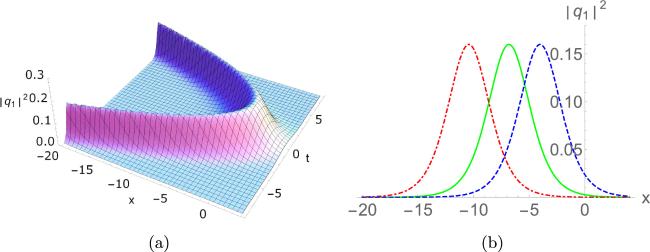
Figure 1. The shape and motion of the envelope of one-soliton solution given by ( |
The soliton ∣q1∣2 travels with a fixed amplitude $A={a}_{1}^{2}$. The top trace of ∣q1∣2 is a parabola, which can be derived as
$\begin{eqnarray}x\,(t)=\displaystyle \frac{{a}_{1}^{3}-3{a}_{1}{\left(\,,{b}_{1}+2\alpha t\right)}^{2}-6\alpha \,({d}_{1}+{f}_{1}\,)+6\alpha \;\mathrm{ln}\,(2{a}_{1})}{6\alpha {a}_{1}},\end{eqnarray}$
of which the vertex point is $\begin{eqnarray*}(x,t)=\left(\displaystyle \frac{{a}_{1}^{3}-6\alpha \,({d}_{1}+{f}_{1}\,)+6\alpha \;\mathrm{ln}\,(2{a}_{1}))}{6\alpha {a}_{1}},-\displaystyle \frac{{b}_{1}}{2\alpha }\right),\end{eqnarray*}$
and the velocity of the soliton is $\begin{eqnarray*}x^{\prime} \,(t)=-2\,(2\alpha t+{b}_{1}).\end{eqnarray*}$
4.2.3. Two-soliton solution
For N = 2 case, we have4.5 ) becomes:
$\begin{eqnarray}{{\boldsymbol{K}}}_{1}=\left(\begin{array}{cc}{k}_{1} & 0\\ 0 & {k}_{2}\end{array}\right),\,\,\,\,{{\boldsymbol{r}}}_{1}={\left({\rho }_{1},{\rho }_{2}\,\right)}^{{\rm{T}}},\,\,\,\,{{\boldsymbol{s}}}_{1}={\left({\sigma }_{1},{\sigma }_{2}\,\right)}^{{\rm{T}}},\end{eqnarray}$
and the dressed Cauchy matrix comes to be $\begin{eqnarray*}{{\boldsymbol{M}}}_{1}=\left(\begin{array}{cc}\displaystyle \frac{{\rho }_{1}\,{\sigma }_{1}^{* }}{{k}_{1}+{k}_{1}^{* }} & \displaystyle \frac{{\rho }_{1}\,{\sigma }_{2}^{* }}{{k}_{1}+{k}_{2}^{* }}\\ \displaystyle \frac{{\rho }_{2}\,{\sigma }_{1}^{* }}{{k}_{2}+{k}_{1}^{* }} & \displaystyle \frac{{\rho }_{2}\,{\sigma }_{2}^{* }}{{k}_{2}+{k}_{2}^{* }}\end{array}\right).\end{eqnarray*}$
Then the explicit formula of the two-soliton solution ( $\begin{eqnarray}{q}_{1}=\displaystyle \frac{(1+{M}_{11})\,{{\rm{e}}}^{{\zeta }_{2}+{\xi }_{2}}-{M}_{12}\,{{\rm{e}}}^{{\zeta }_{1}+{\xi }_{2}}-{M}_{21}\,{{\rm{e}}}^{{\zeta }_{2}+{\xi }_{1}}+(1+{M}_{22})\,{{\rm{e}}}^{{\zeta }_{1}+{\xi }_{1}\,}}{1+{M}_{11}-{M}_{12}\,{M}_{21}+{M}_{22}\,(1+{M}_{11})},\end{eqnarray}$
where $\begin{eqnarray*}\begin{array}{l}\left(\begin{array}{cc}{M}_{11} & {M}_{12}\\ {M}_{21} & {M}_{22}\end{array}\right)=\left(\begin{array}{cc}\displaystyle \frac{{{\rm{e}}}^{2\;\mathrm{Re}\,[{\xi }_{1}+{\zeta }_{1}]\,}}{4{a}_{1}^{2}}+\displaystyle \frac{{{\rm{e}}}^{{\xi }_{1}+{\zeta }_{1}+{\xi }_{2}^{* }+{\zeta }_{2}^{* }}}{{B}^{2}} & \displaystyle \frac{1}{2}{{\rm{e}}}^{{\zeta }_{2}+{\xi }_{1}}\,\left(\displaystyle \frac{{{\rm{e}}}^{{\xi }_{1}^{* }+{\zeta }_{1}^{* }}}{{a}_{1}\,{B}^{* }}+\displaystyle \frac{{{\rm{e}}}^{{\xi }_{2}^{* }+{\zeta }_{2}^{* }}}{{a}_{2}\,B}\right)\\ \displaystyle \frac{1}{2}{{\rm{e}}}^{{\zeta }_{1}+{\xi }_{2}}\,\left(\displaystyle \frac{{{\rm{e}}}^{{\xi }_{1}^{* }+{\zeta }_{1}^{* }}}{{a}_{1}\,{B}^{* }}+\displaystyle \frac{{{\rm{e}}}^{{\xi }_{2}^{* }+{\zeta }_{2}^{* }}}{{a}_{2}\,B}\right) & \displaystyle \frac{{{\rm{e}}}^{2\;\mathrm{Re}\,[{\xi }_{2}+{\zeta }_{2}]\,}}{4{a}_{2}^{2}}+\displaystyle \frac{{{\rm{e}}}^{{\xi }_{2}+{\zeta }_{2}+{\xi }_{1}^{* }+{\zeta }_{1}^{* }}}{{\left({B}^{* }\right)}^{2}}\end{array}\right),\\ B={c}_{1}+{c}_{2}^{* }={a}_{1}+{a}_{2}+{\rm{i}}\,({b}_{1}-{b}_{2}).\end{array}\end{eqnarray*}$
For the shape and motion of ∣q1∣2, we illustrate them in figure 2.
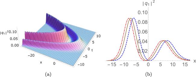
Figure 2. The shape and motion of the two-soliton solution given by ∣q1∣2 with ( |
4.2.4. Double-pole solution
The matrix K1 can also be a triangle Toeplitz matrix (see appendix A ), which will lead to the so-called multiple-pole solutions. We will present solution formula in appendix A for the Sylvester equations in (2.3 ) where K1 and K2 are triangular Toeplitz matrices. For the double-pole solution, it can be obtained by setting4.10 ). Then the dressed Cauchy matrix can be constructed via appendix A as4.5 ) reads
$\begin{eqnarray}\begin{array}{l}{{\boldsymbol{K}}}_{1}=\left(\begin{array}{cc}{k}_{1} & 0\\ {\partial }_{{c}_{1}}\,{k}_{1} & {k}_{1}\end{array}\right),\,\,\,\,{{\boldsymbol{r}}}_{1}={\left({\rho }_{1},{\partial }_{{c}_{1}}\,{\rho }_{1}\,\right)}^{{\rm{T}}},\,\,\,\,{{\boldsymbol{s}}}_{1}\\ ={\left({\sigma }_{1},{\partial }_{{c}_{1}}\,{\sigma }_{1}\,\right)}^{{\rm{T}}},\end{array}\end{eqnarray}$
where k1, ρ1, σ1 are defined as in ( $\begin{eqnarray}{{\boldsymbol{M}}}_{1}=\left(\begin{array}{cc}{\rho }_{1} & 0\\ {\partial }_{{c}_{1}}\,{\rho }_{1} & {\rho }_{1}\end{array}\right)\,\left(\begin{array}{cc}\displaystyle \frac{1}{{k}_{1}+{k}_{1}^{* }} & -\displaystyle \frac{{\left({\partial }_{{c}_{1}}\,{k}_{1}\right)}^{* }}{{\left({k}_{1}+{k}_{1}^{* }\right)}^{2}}\\ -\displaystyle \frac{{\partial }_{{c}_{1}}\,{k}_{1}}{{\left({k}_{1}+{k}_{1}^{* }\right)}^{2}} & \displaystyle \frac{2\,({\partial }_{{c}_{1}}\,{k}_{1})\,{\left({\partial }_{{c}_{1}}\,{k}_{1}\right)}^{* }}{{\left({k}_{1}+{k}_{1}^{* }\right)}^{3}}\end{array}\right)\,\left(\begin{array}{cc}{\sigma }_{1}^{* } & {\left({\partial }_{{c}_{1}}\,{\sigma }_{1}\right)}^{* }\\ {\left({\partial }_{{c}_{1}}\,{\sigma }_{1}\right)}^{* } & 0\end{array}\right).\end{eqnarray}$
The explicit formula of the double-pole solution ( $\begin{eqnarray}{q}_{1}=\displaystyle \frac{16{a}_{1}^{3}\,{{\rm{e}}}^{{\xi }_{1}+{\zeta }_{1}}\left(\,,16{a}_{1}^{5}\,(1+{D}^{2})-({a}_{1}-2{D}^{* }+{a}_{1}{\left(\,,{D}^{2}\right)}^{* })\,{D}^{2}{{\rm{e}}}^{2\;\mathrm{Re}\,[{\xi }_{1}+{\zeta }_{1}]\,}\right)}{256{a}_{1}^{8}+32{A}_{1}\,{a}_{1}^{4}\,{{\rm{e}}}^{2\;\mathrm{Re}\,[{\xi }_{1}+{\zeta }_{1}]}+| D{| }^{4}{{\rm{e}}}^{4\;\mathrm{Re}\,[{\xi }_{1}+{\zeta }_{1}]\,}},\end{eqnarray}$
where $\begin{eqnarray*}\begin{array}{l}{A}_{1}=\left(3| D{| }^{2}-4{a}_{1}\;\mathrm{Re}\,[{\rm{D}}]\,(1+| D{| }^{2})\right.\\ \left.+2{a}_{1}^{2}\,(1+{D}^{2})\,(1+{\left({D}^{2}\right)}^{* })\right),\\ D=\displaystyle \frac{x}{2}-\displaystyle \frac{{k}_{1}^{2}}{4\alpha }.\end{array}\end{eqnarray*}$
The shape and motion of ∣q1∣2 are illustrated in figure 3.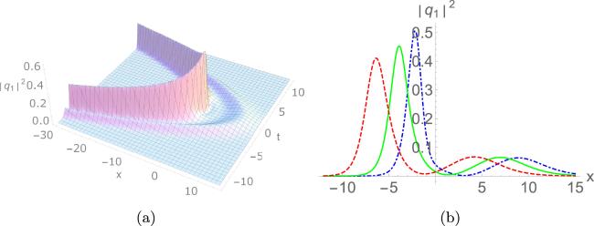
Figure 3. The shape and motion of the double-pole soliton ∣q1∣2 with ( |
4.3. Explicit solutions of the NNLSE-II and dynamics
4.3.1. Formulation of solitons
Solution q2 of the NNLSE-II equation (1.2b ) can be expressed through (4.5 ) where M1, r1, s1 are determined by
$\begin{eqnarray}{{\boldsymbol{K}}}_{1}\,{{\boldsymbol{M}}}_{1}+{{\boldsymbol{M}}}_{1}\,{{\boldsymbol{K}}}_{1}^{* }={{\boldsymbol{r}}}_{1}\,{{\boldsymbol{s}}}_{1}^{\dagger },\end{eqnarray}$
$\begin{eqnarray}{{\boldsymbol{r}}}_{1,x}=\displaystyle \frac{1}{2}{{\boldsymbol{K}}}_{1}\,{{\boldsymbol{r}}}_{1},\,\,\,\,{{\boldsymbol{s}}}_{1,x}=\displaystyle \frac{1}{2}{{\boldsymbol{K}}}_{1}^{{\rm{T}}}\,{{\boldsymbol{s}}}_{1},\end{eqnarray}$
$\begin{eqnarray}\begin{array}{l}{{\boldsymbol{r}}}_{1,t}=-\displaystyle \frac{1}{2}\left(\,,{\rm{i}}{{\boldsymbol{K}}}_{1}^{2}+\beta x{{\boldsymbol{K}}}_{1}+\beta ,\,\right){{\boldsymbol{r}}}_{1},\\ {{\boldsymbol{s}}}_{1,t}=-\displaystyle \frac{1}{2}\left(\,,{\rm{i}}{\left(\,,{{\boldsymbol{K}}}_{1}^{{\rm{T}}}\,\right)}^{2}+\beta x{{\boldsymbol{K}}}_{1}^{{\rm{T}}}+\beta ,\,\right){{\boldsymbol{s}}}_{1},\end{array}\end{eqnarray}$
and $\begin{eqnarray}{{\boldsymbol{K}}}_{1,t}=-\beta {{\boldsymbol{K}}}_{1}\,(t),\,\,\beta \in {\mathbb{R}}.\end{eqnarray}$
In the case of K1 being a diagonal matrix (4.8 ), r1, s1, M1 are given as (4.9 ) where
$\begin{eqnarray}{k}_{j}\,(t)={c}_{j}\,{{\rm{e}}}^{-\beta t},\end{eqnarray}$
$\begin{eqnarray}{\rho }_{j}={{\rm{e}}}^{{\xi }_{j}},\,\,{\xi }_{j}=\displaystyle \frac{1}{2}{{xk}}_{j}\,(t)+\displaystyle \frac{{\rm{i}}{k}_{j}^{2}\,(t)}{4\beta }-\displaystyle \frac{\beta }{2}t+{\xi }_{j}^{(0)},\end{eqnarray}$
$\begin{eqnarray}{\sigma }_{j}={{\rm{e}}}^{{\zeta }_{j}},\,\,{\zeta }_{j}=\displaystyle \frac{1}{2}{{xk}}_{j}\,(t)+\displaystyle \frac{{\rm{i}}{k}_{j}^{2}\,(t)}{4\beta }-\displaystyle \frac{\beta }{2}t+{\zeta }_{j}^{(0)}.\end{eqnarray}$
4.3.2. One-soliton solution
The one-soliton solution corresponds to the N = 1 case, in which we have4.21 ). Substituting them into (4.5 ) one obtains4.25 ) describes a solitary wave traveling with an amplitude ${a}_{1}^{2}\,{{\rm{e}}}^{-2\beta t}$, top trace4.26 ) we can also find that when $\left(\mathrm{ln}\;\left(2{a}_{1}\right)-\left({d}_{1}+{f}_{1}\right)\right)={b}_{1}\,=\,0$, there is x(t) = 0, which corresponds to a stationary soliton as shown in figure 4. Note that the non-isospectral effects affect amplitude, velocity and shape of (4.25 ).
$\begin{eqnarray}{{\boldsymbol{K}}}_{1}={k}_{1},\,\,\,\,{{\boldsymbol{r}}}_{1}={\rho }_{1}={{\rm{e}}}^{{\xi }_{1}},\,\,\,\,{{\boldsymbol{s}}}_{1}={\sigma }_{1}={{\rm{e}}}^{{\zeta }_{1}},\,\,\,\,{{\boldsymbol{M}}}_{1}=\displaystyle \frac{{\rho }_{1}\,{\sigma }_{1}^{* }}{{k}_{1}+{k}_{1}^{* }},\end{eqnarray}$
where k1, ρ1, σ1 are defined as in ( $\begin{eqnarray}{q}_{2}=\displaystyle \frac{4{a}_{1}^{2}\,{{\rm{e}}}^{{\xi }_{1}+{\zeta }_{1}\,}}{4{a}_{1}^{2}+{{\rm{e}}}^{2\left(\,,\beta t+{\rm{R}}e\,[{\xi }_{1}+{\zeta }_{1}],\,\right)}},\end{eqnarray}$
and then the envelope reads $\begin{eqnarray}| {q}_{2}{| }^{2}={a}_{1}^{2}\,{{\rm{e}}}^{-2t\beta }{\;{\rm{sech}} }^{2}\;\,\left[{a}_{1}\,{{\rm{e}}}^{-\beta t}\,\left(x-\displaystyle \frac{{b}_{1}}{\beta }\right)-\mathrm{ln}\,(2{a}_{1})+{d}_{1}+{f}_{1}\right].\end{eqnarray}$
equation ( $\begin{eqnarray}x\,(t)=\displaystyle \frac{\left(\mathrm{ln}\;\left(2{a}_{1}\right)-\left({d}_{1}+{f}_{1}\,\right),\,\right){{\rm{e}}}^{\beta t}}{{a}_{1}}+\displaystyle \frac{{b}_{1}\,{{\rm{e}}}^{-\beta t}}{\beta }\end{eqnarray}$
and velocity $\begin{eqnarray*}\begin{array}{l}x^{\prime} \,(t)=\displaystyle \frac{\beta \left(\,,\mathrm{ln}\;\left(2{a}_{1}\right)-\left({d}_{1}+{f}_{1}\,\right),\,\right){{\rm{e}}}^{\beta t}}{{a}_{1}}-{b}_{1}\,{{\rm{e}}}^{-\beta t}.\end{array}\end{eqnarray*}$
When $\tfrac{\left(\mathrm{ln}\;\left(2{a}_{1}\right)-\left({d}_{1}+{f}_{1}\,\right)\right)}{{a}_{1}}\tfrac{{b}_{1}}{\beta }\gt 0$, the top trace has a similar shape to $\mathrm{sgn}\,[\tfrac{{b}_{1}}{\beta }]\,\cosh \;\beta t;$ while when $\tfrac{\left(\mathrm{ln}\;\left(2{a}_{1}\right)-\left({d}_{1}+{f}_{1}\,\right)\right)}{{a}_{1}}\tfrac{{b}_{1}}{\beta }\lt 0$, the top trace has a similar shape to $-\mathrm{sgn}\,[\tfrac{{b}_{1}}{\beta }]\,\sinh \;\beta t$. From (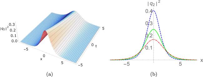
Figure 4. The shape and motion of stationary one-soliton solution given by ( |
4.3.3. Two-soliton solution
When N = 2 we have4.21 ). Then, the explicit formula the two-soliton solution (4.5 ) becomes:
$\begin{eqnarray}\begin{array}{l}{{\boldsymbol{K}}}_{1}=\left(\begin{array}{cc}{k}_{1} & 0\\ 0 & {k}_{2}\end{array}\right),\,\,{{\boldsymbol{r}}}_{1}={\left({\rho }_{1},{\rho }_{2}\,\right)}^{{\rm{T}}},\\ {{\boldsymbol{s}}}_{1}={\left({\sigma }_{1},{\sigma }_{2}\,\right)}^{{\rm{T}}},\,\,{{\boldsymbol{M}}}_{1}=\left(\begin{array}{cc}\displaystyle \frac{{\rho }_{1}\,{\sigma }_{1}^{* }}{{k}_{1}+{k}_{1}^{* }} & \displaystyle \frac{{\rho }_{1}\,{\sigma }_{2}^{* }}{{k}_{1}+{k}_{2}^{* }}\\ \displaystyle \frac{{\rho }_{2}\,{\sigma }_{1}^{* }}{{k}_{2}+{k}_{1}^{* }} & \displaystyle \frac{{\rho }_{2}\,{\sigma }_{2}^{* }}{{k}_{2}+{k}_{2}^{* }}\end{array}\right),\end{array}\end{eqnarray}$
where kj, ρj, σj are defined as in ( $\begin{eqnarray}{q}_{2}=\displaystyle \frac{(1+{H}_{11})\,{{\rm{e}}}^{{\zeta }_{2}+{\xi }_{2}}-{H}_{12}\,{{\rm{e}}}^{{\zeta }_{1}+{\xi }_{2}}-{H}_{21}\,{{\rm{e}}}^{{\zeta }_{2}+{\xi }_{1}}+(1+{H}_{22})\,{{\rm{e}}}^{{\zeta }_{1}+{\xi }_{1}\,}}{1+{H}_{11}-{H}_{12}\,{H}_{21}+{H}_{22}\,(1+{H}_{11})},\end{eqnarray}$
where $\begin{eqnarray*}\begin{array}{l}\left(\begin{array}{cc}{H}_{11} & {H}_{12}\\ {H}_{21} & {H}_{22}\end{array}\right)\\ =\left(\begin{array}{cc}\displaystyle \frac{1}{4}{{\rm{e}}}^{2t\beta +{\zeta }_{1}+{\xi }_{1}}\,\left(\displaystyle \frac{{{\rm{e}}}^{{\zeta }_{1}^{* }+{\xi }_{1}^{* }}}{{a}_{1}^{2}}+\displaystyle \frac{4{{\rm{e}}}^{{\xi }_{2}^{* }+{\zeta }_{2}^{* }}}{{B}^{2}}\right) & \displaystyle \frac{1}{2}{{\rm{e}}}^{2t\beta +{\zeta }_{2}+{\xi }_{1}}\,\left(\displaystyle \frac{{{\rm{e}}}^{{\zeta }_{1}^{* }+{\xi }_{1}^{* }}}{{a}_{1}\,{B}^{* }}+\displaystyle \frac{{{\rm{e}}}^{{\xi }_{2}^{* }+{\zeta }_{2}^{* }}}{{a}_{2}\,B}\right)\\ \displaystyle \frac{1}{2}{{\rm{e}}}^{2t\beta +{\zeta }_{1}+{\xi }_{2}}\,\left(\displaystyle \frac{{{\rm{e}}}^{{\zeta }_{1}^{* }+{\xi }_{1}^{* }}}{{a}_{1}\,{B}^{* }}+\displaystyle \frac{{{\rm{e}}}^{{\xi }_{2}^{* }+{\zeta }_{2}^{* }}}{{a}_{2}\,B}\right) & \displaystyle \frac{1}{4}{{\rm{e}}}^{2t\beta +{\zeta }_{2}+{\xi }_{2}}\,\left(\displaystyle \frac{4{{\rm{e}}}^{{\zeta }_{1}^{* }+{\xi }_{1}^{* }}}{{\left({B}^{* }\right)}^{2}}+\displaystyle \frac{{{\rm{e}}}^{{\xi }_{2}^{* }+{\zeta }_{2}^{* }}}{{a}_{2}^{2}}\right)\end{array}\right),\\ B={c}_{1}+{c}_{2}^{* }={a}_{1}+{a}_{2}+{\rm{i}}\,({b}_{1}-{b}_{2}).\end{array}\end{eqnarray*}$
The shape and motion of ∣q2∣2 are illustrated in figure 5.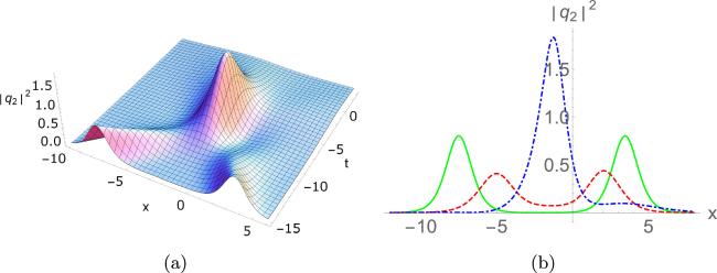
Figure 5. The shape and motion of the envelope of two-soliton solution ( |
4.3.4. Double-pole solution
Double-pole solution of the NNLSE-II can be given by the formula (4.5 ) with the setting (4.17 ) and M1 takes the form (4.18 ), where k1, ρ1, σ1 are defined as in (4.21 ). The explicit formula of such a solution reads
$\begin{eqnarray}{q}_{2}=\displaystyle \frac{16{a}_{1}^{3}\,{{\rm{e}}}^{{\xi }_{1}+{\zeta }_{1}}\left(\,,16{a}_{1}^{5}\,(1+{D}^{2})-{D}^{2}\,({a}_{1}-2{D}^{* }+{a}_{1}{\left(\,,{D}^{2}\right)}^{* })\,{{\rm{e}}}^{2\,(\beta t+\mathrm{Re}\,[{\xi }_{1}+{\zeta }_{1}])\,}\right)}{256{a}_{1}^{8}+32{A}_{1}\,{a}_{1}^{4}\,{{\rm{e}}}^{2\,(\beta t+\mathrm{Re}\,[{\xi }_{1}+{\zeta }_{1}])}+| D{| }^{4}{{\rm{e}}}^{4\,(t\beta +\mathrm{Re}\,[{\xi }_{1}+{\zeta }_{1}])\,}},\end{eqnarray}$
where $\begin{eqnarray*}\begin{array}{l}{A}_{1}=3| D{| }^{2}-4{a}_{1}\;\mathrm{Re}\,[{\rm{D}}]\,(1+| D{| }^{2})+2{a}_{1}^{2}\,(1+{D}^{2})\,(1+{\left({D}^{* }\right)}^{2}),\\ D=\displaystyle \frac{1}{2}x{{\rm{e}}}^{-\beta t}+\displaystyle \frac{{\rm{i}}{c}_{1}\,{{\rm{e}}}^{-2\beta t}}{2\beta }.\end{array}\end{eqnarray*}$
Shape and motion of ∣q2∣2 are illustrated in figure 6.
Figure 6. The shape and motion of the envelope of the double-pole soliton ( |
4.4. Explicit solution of the NNLSE-III and dynamics
4.4.1. Formulation of solitons
For the NNLSE-III equation (1.2c ), its solutions are formulated by (4.5 ) where M1, r1, s1 are determined by
$\begin{eqnarray}{{\boldsymbol{K}}}_{1}\,{{\boldsymbol{M}}}_{1}+{{\boldsymbol{M}}}_{1}\,{{\boldsymbol{K}}}_{1}^{* }={{\boldsymbol{r}}}_{1}\,{{\boldsymbol{s}}}_{1}^{\dagger },\end{eqnarray}$
$\begin{eqnarray}{{\boldsymbol{r}}}_{1,x}=\displaystyle \frac{1}{2}{{\boldsymbol{K}}}_{1}\,{{\boldsymbol{r}}}_{1},\,\,\,\,{{\boldsymbol{s}}}_{1,x}=\displaystyle \frac{1}{2}{{\boldsymbol{K}}}_{1}^{{\rm{T}}}\,{{\boldsymbol{s}}}_{1},\end{eqnarray}$
$\begin{eqnarray}{{\boldsymbol{r}}}_{1,t}=-{\rm{i}}\,\left(\displaystyle \frac{1}{2}x{{\boldsymbol{K}}}_{1}^{2}+{{\boldsymbol{K}}}_{1}\,\right)\,{{\boldsymbol{r}}}_{1},\,\,\,\,{{\boldsymbol{s}}}_{1,t}=-{\rm{i}}\,\left(\displaystyle \frac{1}{2}x{\left(\,,{{\boldsymbol{K}}}_{1}^{{\rm{T}}}\,\right)}^{2}+{{\boldsymbol{K}}}_{1}\,\right)\,{{\boldsymbol{s}}}_{1},\end{eqnarray}$
and $\begin{eqnarray}{{\boldsymbol{K}}}_{1,t}=-{\rm{i}}{{\boldsymbol{K}}}_{1}^{2}.\end{eqnarray}$
In the case of K1 being a diagonal matrix (4.8 ), r1, s1, M1 are given as (4.9 ) where
$\begin{eqnarray}{k}_{j}\,(t)=\displaystyle \frac{1}{{\rm{i}}t-{c}_{j}},\end{eqnarray}$
$\begin{eqnarray}{\rho }_{j}={{\rm{e}}}^{{\xi }_{j}},\,\,{\xi }_{j}=\displaystyle \frac{1}{2}{{xk}}_{j}\,(t)+\mathrm{ln}\,({k}_{j}\,(t))+{\xi }_{j}^{(0)},\end{eqnarray}$
$\begin{eqnarray}{\sigma }_{j}={{\rm{e}}}^{{\zeta }_{j}},\,\,{\zeta }_{j}=\displaystyle \frac{1}{2}{{xk}}_{j}\,(t)+\mathrm{ln}\,({k}_{j}\,(t))+{\zeta }_{j}^{(0)}.\end{eqnarray}$
4.4.2. One-soliton solution
For one-soliton, we have4.32 ). From (4.5 ) we have4.35 ) reads
$\begin{eqnarray}{{\boldsymbol{K}}}_{1}={k}_{1},\quad {{\boldsymbol{r}}}_{1}={\rho }_{1}={{\rm{e}}}^{{\xi }_{1}},\quad {{\boldsymbol{s}}}_{1}={\sigma }_{1}={{\rm{e}}}^{{\zeta }_{1}},\quad {{\boldsymbol{M}}}_{1}=\displaystyle \frac{{\rho }_{1}\,{\sigma }_{1}^{* }}{{k}_{1}+{k}_{1}^{* }},\end{eqnarray}$
where k1, ρ1, σ1 are defined as in ( $\begin{eqnarray}{q}_{3}=\displaystyle \frac{4{a}_{1}^{2}\,{{\rm{e}}}^{{\xi }_{1}+{\zeta }_{1}\,}}{4{a}_{1}^{2}+{\left({a}_{1}^{2}+{\left({b}_{1}-t\right)}^{2}\right)}^{2}{{\rm{e}}}^{2\left(\,,{\rm{R}}e\,[{\xi }_{1}+{\zeta }_{1}],\,\right)}},\end{eqnarray}$
which yields $\begin{eqnarray}\begin{array}{l}| {q}_{3}{| }^{2}=\displaystyle \frac{{a}_{1}^{2}}{{\left({a}_{1}^{2}+{\left({b}_{1}-t\right)}^{2}\right)}^{2}}{\;{\rm{sech}} }^{2}\;\\ \left[{d}_{1}+{f}_{1}-\displaystyle \frac{{a}_{1}\,x}{{a}_{1}^{2}+{\left({b}_{1}-t\right)}^{2}}-\mathrm{ln}\,(2{a}_{1})\,\right].\end{array}\end{eqnarray}$
The envelope is depicted in figure 7. It is interesting that ∣q3∣2 has a time-dependent amplitude $\tfrac{{a}_{1}^{2}}{{\left({a}_{1}^{2}+{\left({b}_{1}-t\right)}^{2}\right)}^{2}}$, which indicates that the soliton is a localized wave with respect to both space and time. In addition, the top trace for ( $\begin{eqnarray*}x\,(t)=\displaystyle \frac{A\,({a}_{1}^{2}+{\left({b}_{1}-t\right)}^{2})}{{a}_{1}},\,\,\mathrm{where}\,\,A={d}_{1}+{f}_{1}-\mathrm{ln}\,(2{a}_{1}),\end{eqnarray*}$
which, in general, is a parabola curve, and along which the soliton travels and changes its direction at the vertex (t, x) = (b1, Aa1) where ∣q3∣2 takes maximum value $\tfrac{1}{{a}_{1}^{2}}$, see, e.g. Figure 7(c). A special case takes place when A = 0, which yields a stationary soliton, as depicted in figure 7(a).
Figure 7. The shape and motion the envelope of one-soliton solution given by ( |
4.4.3. Two-soliton solution
The two-soliton solution is given by (4.5 ) where K1, r1, s1, M1 are given as in (4.27 ) but kj, ρj, σj are defined as in (4.32 ). The solution is written as
$\begin{eqnarray}{q}_{3}=\displaystyle \frac{(1+{F}_{11})\,{{\rm{e}}}^{{\zeta }_{2}+{\xi }_{2}}-{F}_{12}\,{{\rm{e}}}^{{\zeta }_{1}+{\xi }_{2}}-{F}_{21}\,{{\rm{e}}}^{{\zeta }_{2}+{\xi }_{1}}+(1+{F}_{22})\,{{\rm{e}}}^{{\zeta }_{1}+{\xi }_{1}\,}}{1+{F}_{11}-{F}_{12}\,{F}_{21}+{F}_{22}\,(1+{F}_{11})},\end{eqnarray}$
where $\begin{eqnarray*}\begin{array}{l}\left(\begin{array}{cc}{F}_{11} & {F}_{12}\\ {F}_{21} & {F}_{22}\end{array}\right)\\ =\left(\begin{array}{cc}\displaystyle \frac{{{\rm{e}}}^{2\mathrm{Re}[{\xi }_{1}+{\zeta }_{1}]}}{{\left({k}_{1}+{k}_{1}^{* }\right)}^{2}}+\displaystyle \frac{{{\rm{e}}}^{{\xi }_{1}+{\zeta }_{1}+{\zeta }_{2}^{* }+{\xi }_{2}^{* }}}{{\left({k}_{1}+{k}_{2}^{* }\right)}^{2}} & \displaystyle \frac{{{\rm{e}}}^{2\mathrm{Re}[{\xi }_{1}]+{\zeta }_{2}+{\zeta }_{1}^{* }}}{({k}_{1}+{k}_{1}^{* })({k}_{1}^{* }+{k}_{2})}+\displaystyle \frac{{{\rm{e}}}^{2\mathrm{Re}[{\zeta }_{2}]+{\xi }_{1}+{\xi }_{2}^{* }}}{({k}_{1}+{k}_{2}^{* })({k}_{2}+{k}_{2}^{* })}\\ \displaystyle \frac{{{\rm{e}}}^{2\mathrm{Re}[{\zeta }_{1}]+{\xi }_{2}+{\xi }_{1}^{* }}}{({k}_{1}+{k}_{1}^{* })({k}_{1}^{* }+{k}_{2})}+\displaystyle \frac{{{\rm{e}}}^{2\mathrm{Re}[{\xi }_{2}]+{\zeta }_{1}+{\zeta }_{2}^{* }}}{({k}_{1}+{k}_{2}^{* })({k}_{2}+{k}_{2}^{* })} & \displaystyle \frac{{{\rm{e}}}^{2\mathrm{Re}[{\xi }_{2}+{\zeta }_{2}]}}{{\left({k}_{2}+{k}_{2}^{* }\right)}^{2}}+\displaystyle \frac{{{\rm{e}}}^{{\xi }_{1}^{* }+{\zeta }_{1}^{* }+{\zeta }_{2}+{\xi }_{2}}}{{\left({k}_{1}^{* }+{k}_{2}\right)}^{2}}\end{array}\right).\end{array}\end{eqnarray*}$
For the shape and motion of the envelope ∣q3∣2, we illustrate them in figure 8, where (a) shows the scattering of two solitons and (b) describes interactions of two different stationary solitons.
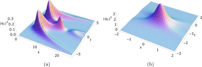
Figure 8. The shape and motion of the envelope of two-soliton solution ( |
4.4.4. Double-pole solution
Double-pole solution of the NNLSE-III is given by the formula (4.5 ) with the setting (4.17 ) and M1 takes the form (4.18 ), where k1, ρ1, σ1 are defined as in (4.32 ). Its explicit formula is
$\begin{eqnarray}{q}_{3}=\displaystyle \frac{\left(1+{R}_{22}-({R}_{12}+{R}_{21})\,V+(1+{R}_{11})\,{V}^{* },\,\right){{\rm{e}}}^{{\xi }_{1}+{\zeta }_{1}\,}}{1+{R}_{11}-{R}_{12}\,{R}_{21}+{R}_{22}+{R}_{11}\,{R}_{22}},\end{eqnarray}$
where $\begin{eqnarray*}V=\displaystyle \frac{1}{2}{k}_{1}^{2}\,x+{k}_{1},\,\,\,\left(\begin{array}{cc}{R}_{11} & {R}_{12}\\ {R}_{21} & {R}_{22}\end{array}\right)={{\boldsymbol{M}}}_{1}\,{{\boldsymbol{M}}}_{1}^{* }.\end{eqnarray*}$
The shape and motion of ∣q3∣2 are illustrated in figure 9. When ${\xi }_{1}^{(0)}\ne {\zeta }_{1}^{(0)}$ we get two solitons moving along the same parabolic top trace, as shown in figure 9(a). When ${\xi }_{1}^{(0)}={\zeta }_{1}^{(0)}=0$ we get two overlapped solitons as shown in figure 9(c).
Figure 9. The shape and motion of the envelope of the double-pole solution ( |
5. Conclusions
In this paper we have developed the Cauchy matrix approach to the NNLSEs, which serve as example models in the ZS-AKNS hierarchy. We believe that solutions of other order equations in the non-isospectral ZS-AKNS hierarchy, such as the non-isospectral sine-Gordon equation, the non-isospectral modified KdV (mKdV) equation and the non-isospectral Hirota equation (combination of the NLS and the mKdV) can be obtained along with this line.
In the Cauchy matrix approach, the Sylvester equation (e.g. (2.1 )) plays an central role, which defines a dressed Cauchy matrix to provide τ functions (i.e. ∣I2N + M∣) for the investigated equations. In non-isospectral case, one needs to suitably select dispersion relations of the time part (e.g. (2.7b ), (2.23b ) and (2.30b )) according to the time-evolution of the spectral parameters. One needs also to formulate special relations (e.g. (2.35 )) to figure out the integration term (e.g. in (2.34 )). Apparently, compared with the isospectral case [23], the non-isospectral extension of the Cauchy matrix scheme is quite non-trivial. In addition, in the isospectral case (see [23]) K is a constant matrix and it can be proved that K and its any similar form lead to same S(i,j) therefore one only needs to consider its canonical form and the resulted solutions can be classified by the canonical forms of K. However, as we have seen that in non-isospectral case K is no longer a constant matrix, usually K and its similar form do not obey the same evolutions (e.g. (2.9 ), (2.24 ) and (2.31 )). Therefore in the non-isospectral case, we can not classify solutions by considering the canonical forms of K. In appendix A we will formulate solutions of the Sylvester equations in (2.3 ) where K1 and K2 are triangular Toeplitz matrices, which are used to get multiple-pole solutions. Note that the Sylvester equation (2.1 ) to formulate the ZS-AKNS system is different from the one for the KdV type and KP type equations (see [22, 27]). Extension of the Cauchy matrix approach to the non-isospectral KdV and KP type equations (as well as the non-isospectral equations with sources, e.g. [30]) will be considered elsewhere.
Appendix A. Solutions to (2.3 ) with triangular Toeplitz matrices
We sketch a procedure to construct solutions to the Sylvester equations in (2.3 ) when K1 and K2 are lower triangular Toeplitz matrices. A lower triangular Toeplitz matrix is a square matrix in the following form and can be considered to be generated by a certain function:
$\begin{eqnarray}{{\boldsymbol{F}}}_{c}^{[N]\,}\left[\,,\,f\,(c)\right]={\left(\begin{array}{ccccc}\,f & 0 & 0 & \cdots & 0\\ \displaystyle \frac{{\partial }_{c}\,f}{1!} & f & 0 & \cdots & 0\\ \displaystyle \frac{{\partial }_{c}^{2}\,f}{2!} & \displaystyle \frac{{\partial }_{c}\,f}{1!} & f & \cdots & 0\\ \vdots & \vdots & \vdots & \ddots & \vdots \\ \displaystyle \frac{{\partial }_{c}^{N-1}\,f}{(N-1)!} & \displaystyle \frac{{\partial }_{c}^{N-2}\,f}{(N-2)!} & \displaystyle \frac{{\partial }_{c}^{N-3}\,f}{(N-3)!} & \cdots & f\,\end{array}\right)}_{N\times N},\end{eqnarray}$
where f(c) is the generating function. Note that the subindex ‘c’ indicates that the lower triangular Toeplitz matrix is generated by taking derivatives with respect to c. We also introduce a symmetric matrix generated by f(c), denoted as $\begin{eqnarray}{{\boldsymbol{H}}}_{c}^{[N]\,}[\,f\,(c)]={\left(\begin{array}{ccccc}\,f & \displaystyle \frac{{\partial }_{c}\,f}{1!} & \displaystyle \frac{{\partial }_{c}^{2}\,f}{2!} & ... & \displaystyle \frac{{\partial }_{c}^{N-1}\,f}{(N-1)!}\\ \displaystyle \frac{{\partial }_{c}\,f}{1!} & \displaystyle \frac{{\partial }_{c}^{2}\,f}{2!} & \displaystyle \frac{{\partial }_{c}^{3}\,f}{3!} & ... & 0\\ \displaystyle \frac{{\partial }_{c}^{2}\,f}{2!} & \displaystyle \frac{{\partial }_{c}^{3}\,f}{3!} & \displaystyle \frac{{\partial }_{c}^{4}\,f}{4!} & ... & 0\\ \vdots & \vdots & \vdots & \ddots & \vdots \\ \displaystyle \frac{{\partial }_{c}^{N-1}\,f}{(N-1)!} & 0 & 0 & ... & 0\end{array}\right)}_{N\times N}.\end{eqnarray}$
As a special property of such two types of matrices, we mention that [26] $\begin{eqnarray}\begin{array}{l}{F}_{c}^{[N]\,}[\,f\,(c)\,g\,(c)]={F}_{c}^{[N]\,}[\,f\,(c)]\,{F}_{c}^{[N]\,}[g\,(c)],\\ {H}_{c}^{[N]\,}[\,f\,(c)\,g\,(c)]={H}_{c}^{[N]\,}[\,f\,(c)]\,{F}_{c}^{[N]\,}[g\,(c)].\end{array}\end{eqnarray}$
For more properties, one can refer to [29] and proposition 3 in [26].In the following we will use the notations k1, l1, ρ1, ϱ1, σ1 and ϖ1 that we introduced in section 3 but we do not specify them since the following description is generic and true for all the three NNLSEs. We consider k1 and l1 to be functions of c1 and d1, respectively, e.g. (3.2 ), (3.9 ) and (3.11 ). Let2.9 ), (2.24 ) and (2.31 ) when k1, l1 are defined as (3.2 ), (3.9 ) and (3.11 ), respectively. Next, define2.7 ), (2.23 ) and (2.30 ) when k1, l1 are defined as (3.2 ), (3.9 ) and (3.11 ), respectively.
$\begin{eqnarray}{{\boldsymbol{K}}}_{1}={{\boldsymbol{F}}}_{{c}_{1}}^{[N]\,}\left[\,,{k}_{1}\right],\,\,{{\boldsymbol{K}}}_{2}={{\boldsymbol{F}}}_{{d}_{1}}^{[N]\,}\left[\,,{l}_{1}\right].\end{eqnarray}$
Then, it can be verified that K = diag(K1, K2) satisfies the evolutions ( $\begin{eqnarray}{{\boldsymbol{r}}}_{1}={{\boldsymbol{F}}}_{1}\,{{\boldsymbol{e}}}_{N},\,\,\,\,{{\boldsymbol{s}}}_{2}={{\boldsymbol{H}}}_{2}\,{{\boldsymbol{e}}}_{N},\,\,\,\,{{\boldsymbol{F}}}_{1}={{\boldsymbol{F}}}_{{c}_{1}}^{[N]\,}\left[\,,{\rho }_{1}\right],\,\,\,\,{{\boldsymbol{H}}}_{2}={{\boldsymbol{H}}}_{{d}_{1}}^{[N]\,}\left[\,,{\varpi }_{1}\right],\end{eqnarray}$
$\begin{eqnarray}{{\boldsymbol{r}}}_{2}={{\boldsymbol{F}}}_{2}\,{{\boldsymbol{e}}}_{N},\,\,\,\,{{\boldsymbol{s}}}_{1}={{\boldsymbol{H}}}_{1}\,{{\boldsymbol{e}}}_{N},\,\,\,\,{{\boldsymbol{F}}}_{2}={{\boldsymbol{F}}}_{{d}_{1}}^{[N]\,}\left[\,,{\varrho }_{1}\right],\,\,\,\,{{\boldsymbol{H}}}_{1}={{\boldsymbol{H}}}_{{c}_{1}}^{[N]\,}\left[\,,{\sigma }_{1}\right],\end{eqnarray}$
where $\begin{eqnarray*}{{\boldsymbol{e}}}_{N}={\left(\mathop{\underbrace{\mathrm{1,0,0},\cdots ,0}}\limits_{N-\mathrm{dimensional}}\right)}^{{\rm{T}}}.\end{eqnarray*}$
Then, the above defined elements satisfy the dispersion relations (Next, we look for solution M1 and M2 of the Sylvester equations in (2.3 ) in the form2.3a ) can be rewritten asA.6 ) reduces toA.7 ) readsA.7 ), which is
$\begin{eqnarray}{{\boldsymbol{M}}}_{1}={{\boldsymbol{F}}}_{1}\,{{\boldsymbol{G}}}_{1}\,{{\boldsymbol{H}}}_{2},\,\,\,\,{{\boldsymbol{M}}}_{2}={{\boldsymbol{F}}}_{2}\,{{\boldsymbol{G}}}_{2}\,{{\boldsymbol{H}}}_{1},\end{eqnarray}$
where G1 and G2 are unknowns. In these settings, equation ( $\begin{eqnarray}{{\boldsymbol{K}}}_{1}\,{{\boldsymbol{F}}}_{1}\,{{\boldsymbol{G}}}_{1}\,{{\boldsymbol{H}}}_{2}-{{\boldsymbol{F}}}_{1}\,{{\boldsymbol{G}}}_{1}\,{{\boldsymbol{H}}}_{2}\,{{\boldsymbol{K}}}_{2}={{\boldsymbol{F}}}_{1}\,{{\boldsymbol{e}}}_{N}\,{{\boldsymbol{e}}}_{N}^{{\rm{T}}}\,{{\boldsymbol{H}}}_{2}.\end{eqnarray}$
Using the relations [26] $\begin{eqnarray*}{{\boldsymbol{K}}}_{1}\,{{\boldsymbol{F}}}_{1}={{\boldsymbol{F}}}_{1}\,{{\boldsymbol{K}}}_{1},\,\,\,{{\boldsymbol{H}}}_{2}\,{{\boldsymbol{K}}}_{2}={{\boldsymbol{K}}}_{2}^{{\rm{T}}}\,{{\boldsymbol{H}}}_{2}.\end{eqnarray*}$
( $\begin{eqnarray}{{\boldsymbol{K}}}_{1}\,{{\boldsymbol{G}}}_{1}-{{\boldsymbol{G}}}_{1}\,{{\boldsymbol{K}}}_{2}^{{\rm{T}}}={{\boldsymbol{e}}}_{N}\,{{\boldsymbol{e}}}_{N}^{{\rm{T}}}.\end{eqnarray}$
For convenience, we write G1 = (g1, g2, …, gN) where ${{\boldsymbol{g}}}_{j}={({g}_{1,j},{g}_{2,j},\cdots ,{g}_{N,j})}^{{\rm{T}}}$. Then, the first column of ( $\begin{eqnarray*}\left(\begin{array}{c}{k}_{1}\,{g}_{\mathrm{1,1}}\\ ({\partial }_{{c}_{1}}\,{k}_{1})\,{g}_{\mathrm{1,1}}+{k}_{1}\,{g}_{\mathrm{2,1}}\\ \displaystyle \frac{1}{2!}\,({\partial }_{{c}_{1}\,}^{2}\,{k}_{1})\,{g}_{\mathrm{1,1}}+({\partial }_{{c}_{1}}\,{k}_{1})\,{g}_{\mathrm{2,1}}+{k}_{1}\,{g}_{\mathrm{3,1}}\\ \vdots \\ \displaystyle \frac{1}{(N-1)!}\,({\partial }_{{c}_{1}\,}^{N-1}\,{k}_{1})\,{g}_{\mathrm{1,1}}+\;\cdots \;+{k}_{1}\,{g}_{N,1}\end{array}\right)-{l}_{1}\,\left(\begin{array}{c}{g}_{\mathrm{1,1}}\\ {g}_{\mathrm{2,1}}\\ {g}_{\mathrm{3,1}}\\ \vdots \\ {g}_{N,1}\end{array}\right)=\left(\begin{array}{c}1\\ 0\\ 0\\ \vdots \\ 0\end{array}\right),\end{eqnarray*}$
which gives rise to $\begin{eqnarray}{g}_{\mathrm{1,1}}=\displaystyle \frac{1}{{k}_{1}-{l}_{1}},\,\,\,\,{g}_{m,1}=-\displaystyle \frac{1}{{k}_{1}-{l}_{1}}\,\left(\displaystyle \sum _{j=1}^{m-1}\,\displaystyle \frac{{\partial }_{{c}_{1}\,}^{j}\,{k}_{1}}{j!}\,{g}_{m-j,1}\right),\,\,\,\,m=2,3,\cdots ,N,\end{eqnarray}$
from which one can successively determine g2,1, g3,1, ..., gN,1. For example, we have $\begin{eqnarray*}\begin{array}{l}{g}_{\mathrm{2,1}}=-\displaystyle \frac{{\partial }_{{c}_{1}}\,{k}_{1}}{{\left({k}_{1}-{l}_{1}\,\right)}^{2}},\,\,{g}_{\mathrm{3,1}}\\ =\,\displaystyle \frac{{\left({\partial }_{{c}_{1}}\,{k}_{1}\,\right)}^{2}}{{\left({k}_{1}-{l}_{1}\,\right)}^{3}}\\ -\,\displaystyle \frac{{\partial }_{{c}_{1}\,}^{2}\,{k}_{1}}{2!{\left({k}_{1}-{l}_{1}\,\right)}^{2}}.\end{array}\end{eqnarray*}$
Once with g1 in hand, we can look at the second column of ( $\begin{eqnarray*}\begin{array}{l}\left(\begin{array}{c}{k}_{1}\,{g}_{\mathrm{1,2}}\\ ({\partial }_{{c}_{1}}\,{k}_{1})\,{g}_{\mathrm{1,2}}+{k}_{1}\,{g}_{\mathrm{2,2}}\\ \displaystyle \frac{1}{2!}\,({\partial }_{{c}_{1}\,}^{2}\,{k}_{1})\,{g}_{\mathrm{1,2}}+({\partial }_{{c}_{1}}\,{k}_{1})\,{g}_{\mathrm{2,2}}+{k}_{1}\,{g}_{\mathrm{3,2}}\\ \vdots \\ \displaystyle \frac{1}{(N-1)!}\,({\partial }_{{c}_{1}\,}^{N-1}\,{k}_{1})\,{g}_{\mathrm{1,2}}+\;\cdots \;+{k}_{1}\,{g}_{N,2}\end{array}\right)\\ -\left(\begin{array}{c}({\partial }_{{d}_{1}}\,{l}_{1})\,{g}_{\mathrm{1,1}}+{l}_{1}\,{g}_{\mathrm{1,2}}\\ ({\partial }_{{d}_{1}}\,{l}_{1})\,{g}_{\mathrm{2,1}}+{l}_{1}\,{g}_{\mathrm{2,2}}\\ ({\partial }_{{d}_{1}}\,{l}_{1})\,{g}_{\mathrm{3,1}}+{l}_{1}\,{g}_{\mathrm{3,2}}\\ \vdots \\ ({\partial }_{{d}_{1}}\,{l}_{1})\,{g}_{N,1}+{l}_{1}\,{g}_{N,2}\end{array}\right)\,=\,\left(\begin{array}{c}0\\ 0\\ 0\\ \vdots \\ 0\end{array}\right).\end{array}\end{eqnarray*}$
Element of g2 can be calculated as: $\begin{eqnarray}\begin{array}{l}{g}_{\mathrm{1,2}}=\displaystyle \frac{1}{{k}_{1}-{l}_{1}}\,({\partial }_{{d}_{1}}\,{l}_{1})\,{g}_{\mathrm{1,1}},\,\,{g}_{m,2}\\ =\displaystyle \frac{1}{{k}_{1}-{l}_{1}}\left(\,,\Space{0ex}{3.85ex}{0ex}({\partial }_{{d}_{1}}\,{l}_{1})\,{g}_{m,1}\right.\\ \left.-\displaystyle \sum _{j=1}^{m-1}\,\displaystyle \frac{{\partial }_{{c}_{1}\,}^{j}\,{k}_{1}}{j!}\,{g}_{m-j,2}\right),\,\,m=2,3,\cdots ,N.\end{array}\end{eqnarray}$
The first few elements are $\begin{eqnarray*}\begin{array}{l}{g}_{\mathrm{1,2}}=\displaystyle \frac{{\partial }_{{d}_{1}}\,{l}_{1}}{{\left({k}_{1}-{l}_{1}\,\right)}^{2}},\,\,{g}_{\mathrm{2,2}}=-\displaystyle \frac{2\,({\partial }_{{c}_{1}}\,{k}_{1})\,({\partial }_{{d}_{1}}\,{l}_{1})}{{\left({k}_{1}-{l}_{1}\,\right)}^{3}},\\ {g}_{\mathrm{3,2}}=\displaystyle \frac{3{\left(\,,{\partial }_{{c}_{1}}\,{k}_{1}\,\right)}^{2}\,({\partial }_{{d}_{1}}\,{l}_{1})}{{\left({k}_{1}-{l}_{1}\,\right)}^{4}}\\ -\displaystyle \frac{({\partial }_{{c}_{1}\,}^{2}\,{k}_{1})\,({\partial }_{{d}_{1}}\,{l}_{1})}{{\left({k}_{1}-{l}_{1}\,\right)}^{3}}.\end{array}\end{eqnarray*}$
For the n-th column (n > 1) of (A.7 ), we have
$\begin{eqnarray*}{{\boldsymbol{K}}}_{1}\,{{\boldsymbol{g}}}_{n}-\displaystyle \sum _{j=1}^{n-1}\,\displaystyle \frac{{\partial }_{{d}_{1}\,}^{j}\,{l}_{1}}{j!}{{\boldsymbol{g}}}_{n-j}-{l}_{1}\,{{\boldsymbol{g}}}_{n}=0,\end{eqnarray*}$
which indicates that $\begin{eqnarray*}{{\boldsymbol{g}}}_{n}=\displaystyle \sum _{j=1}^{n-1}\,\displaystyle \frac{{\partial }_{{d}_{1}\,}^{j}\,{l}_{1}}{j!}{\left(\,,{{\boldsymbol{K}}}_{1}-{l}_{1}\,{{\boldsymbol{I}}}_{N}\right)}^{-1}{{\boldsymbol{g}}}_{n-l}.\end{eqnarray*}$
Finally, G1 = (g1, g2, …, gN) can be derived.G2 can be solved from equation (2.3b ) in a similar way. Here we skip the details.