Hybrid rogue waves and breather solutions on the double-periodic background for the Kundu-DNLS equation

DongZhu Jiang; Zhaqilao

doi:10.1088/1572-9494/ad2f24

Communications in Theoretical Physics >

2024 , Vol. 76 >Issue 5: 55003

DOI: https://doi.org/10.1088/1572-9494/ad2f24

Mathematical Physics

Hybrid rogue waves and breather solutions on the double-periodic background for the Kundu-DNLS equation

DongZhu Jiang ^,¹^,² ,
Zhaqilao ^,¹^,²^,^∗

Expand

¹College of Mathematics Science, Inner Mongolia Normal University, Hohhot 010022, China
²Center for Applied Mathematical Science, Inner Mongolia, Hohhot 010022, China

^∗Author to whom any correspondence should be addressed.

Received date: 2023-10-14

Revised date: 2024-02-22

Accepted date: 2024-03-01

Online published: 2024-04-22

Copyright

Fold

Abstract

In this paper, by using the Darboux transformation (DT) method and the Taylor expansion method, a new nth-order determinant of the hybrid rogue waves and breathers solution on the double-periodic background of the Kundu-DNLS equation is constructed when n is even. Breathers and rogue waves can be obtained from this determinant, respectively. Further to this, the hybrid rogue waves and breathers solutions on the different periodic backgrounds are given explicitly, including the single-periodic background, the double-periodic background and the plane wave background by selecting different parameters. In addition, the form of the obtained solutions is summarized.

Key words： double-periodic background; hybrid rogue waves and breather; darboux transformation; Kundu-DNLS equation

Cite this article

DongZhu Jiang , Zhaqilao . Hybrid rogue waves and breather solutions on the double-periodic background for the Kundu-DNLS equation[J]. Communications in Theoretical Physics, 2024 , 76(5) : 055003 . DOI: 10.1088/1572-9494/ad2f24

1. Introduction

Nonlinear phenomena can be seen everywhere in nature. In order to better observe nonlinear phenomena, we have done a lot of research on three important nonlinear wave solutions: soliton, breather and rogue waves [1–5]. It is generally accepted that solitons are the result of nonlinearity and dispersion equilibrium [6], and that rogue waves and breathers are special cases of solitons [7]. Breathers can periodically propagate with a sustained and stable energy, and nondegenerate breathers are constructed in a Manakov system [8–13]. Rogue waves are considered to be the limit of the breather, and occur in both shallow and deep seas [14], which will bring many disasters to the ocean [15]. Many methods have been applied to find breather and rogue waves, such as the Hirota bilinear method [16], Lie Group method [17], Riemann–Hilbert method [18] and DT method [19–21]. Among them, the DT method is an effective way to construct solutions for integrable systems, which originate from Darboux’s 1882 paper on the study of Sturm–Liouville equations. In addition, it is found that nonlinear effects generate higher energies when they collide with each other [7], the work on hybrid rogue waves and breather solutions of partial differential equations (PDEs) has attracted attention, such as the hybrid rogue wave and breather solutions for a complex mKdV equation in few-cycle ultra-short pulse optics [22]. The interaction between solitons and lump solutions is constructed [23, 24]. A hybrid structure of solitons and breathers is constructed [25]. The hybrid structures of solitons, lump solutions and rogue waves are constructed by using the Hirota bilinear method [26, 27]. A hybrid structure of solitons and breathers is constructed [28]. Extended DT has been used to study hybrid rogue waves and breather waves [29–31], which can describe the interaction between the current-fed string and the external magnetic field and other physical phenomena [32]. Therefore, it is very important to study hybrid rogue waves and breather waves.

In general, these solutions are constructed on the plane wave background. However, in real life, the interaction of these solutions is often influenced by other waves, such as periodic waves [33]. When the plane wave background is extended to the periodic background, more properties of the solutions will be revealed. On the basis of these solutions [34–39], some hybrid solutions of nonlinear waves on the periodic background have been constructed, DT and semi-degenerate DT are used to construct the hybrid breather-rogue wave of derivative nonlinear Schrödinger equation (DNLS) on the periodic background [40]. DT and semi-degenerate DTs are used to construct the hybrid breather-rogue waves of the reverse-space-time modified NLS equation on the double-periodic background [41]. By comparison, we find that the properties of the solutions on the double-periodic background are more complex than those on the single-periodic background [41]. It is necessary to study the hybrid solutions on the double-periodic background.

The Kaup–Newell (KN) system is important in a soliton and integrable system, one of the earliest put forward by Kaup and Newell in [42]. On this basis, it is well known that the DNLS equation

(1)$\begin{eqnarray}{\rm{i}}{q}_{t}+{q}_{{xx}}+{\rm{i}}\alpha {(| q{| }^{2}q)}_{x}=0.\end{eqnarray}$

In addition, the Chen–Li–Liu (CLL) equation and Gerdjikov–Ivanov (GI) equation can also be obtained through the KN system, and the modulation instability including super-regular breathers and Akhmediev breathers of the CLL equation have been studied analytically [43, 44]. In physical systems, higher-order nonlinearity is very important, so we get an integrable higher-order nonlinear equation based on equation (1) when q = Q(x, t)e^iθ, namely the Kundu-DNLS equation [45, 46].

(2)$\begin{eqnarray}{\rm{i}}{Q}_{t}+{Q}_{{xx}}+{\rm{i}}\alpha {({Q}^{2}{Q}^{* })}_{x}-({\theta }_{t}+{\theta }_{x}^{2}-{\rm{i}}{\theta }_{{xx}})Q+{\theta }_{x}(2{\rm{i}}{Q}_{x}-\alpha {Q}^{2}{Q}^{* })=0,\end{eqnarray}$

where θ = θ(x, t) is a arbitrary gauge function, Q^* denotes the complex conjugate of Q, and a is a real parameter. For example, setting $\theta =\delta \int Q({x}^{{\prime} }){{dx}}^{{\prime} }$, Kundu-DNLS equation implies the Eckhaus–Kundu (EK) equation [45].

We consider the coupled Kundu-DNLS equation

(3)$\begin{eqnarray}\begin{array}{l}{\rm{i}}{Q}_{t}+{Q}_{{xx}}-{\rm{i}}\alpha {\left({Q}^{2}R\right)}_{x}-\left({\theta }_{t}+{\theta }_{x}^{2}-{\rm{i}}{\theta }_{{xx}}\right)Q+{\theta }_{x}\left(2{\rm{i}}{Q}_{x}+\alpha {Q}^{2}R\right)=0,\\ {\rm{i}}{R}_{t}-{R}_{{xx}}-{\rm{i}}\alpha {\left({R}^{2}Q\right)}_{x}+\left({\theta }_{t}+{\theta }_{x}^{2}+{\rm{i}}{\theta }_{{xx}}\right)R+{\theta }_{x}\left(2{\rm{i}}{R}_{x}-\alpha {R}^{2}Q\right)=0,\end{array}\end{eqnarray}$

the equation (3) can be reduced to the equation (1) when R(x, t) = − Q^*(x, t).

The DNLS equation has been studied by researchers from many aspects, several exact solutions have been constructed by using the DT method in [47], and the solutions on the single- or the double-periodic background of the DNLS equation are obtained in [48]. For the Kundu-DNLS equation, the rogue wave solutions, soliton solutions, positon solutions and breather solutions are constructed in 2013 [49]. However, there has not been much research on the construction of hybrid solutions on the periodic background for the Kundu-DNLS equation.

The paper is organized as follows. In section 2, the Lax pair and the n-transformed solutions of equation (3) are given. In section 3, based on the plane wave seed solution, the nonzero solution of the Lax pair is constructed. By introducing several mathematical methods, we lay the foundation for the construction of subsequent solutions of the equation (3). In section 4, according to section 3, we construct the nth-order determinant representation for finding hybrid rogue waves and breathers solution on the single-periodic background when n is odd. In section 5, according to section 3, we construct the nth-order determinant representation for finding hybrid rogue waves and breathers solution on the double-periodic background when n is even. In section 6, the form of the obtained solutions is summarized. Finally, some conclusions are given.

2. Lax pair and n-transformed solutions of the equation (3)

Based on the KN system [50, 51], equation (3) possesses the Lax pair as

(4)$\begin{eqnarray}\left\{\begin{array}{l}{{\rm{\Phi }}}_{x}=U{\rm{\Phi }}\\ {{\rm{\Phi }}}_{t}=V{\rm{\Phi }}\end{array}\right.,\end{eqnarray}$

where

$\begin{eqnarray*}\begin{array}{l}U=\left(\begin{array}{ll}\displaystyle \frac{{\rm{i}}}{4}{\lambda }^{2} & \displaystyle \frac{{\rm{i}}\sqrt{\alpha }R}{2}\lambda {{\rm{e}}}^{-{\rm{i}}\theta }\\ \displaystyle \frac{{\rm{i}}\sqrt{\alpha }Q}{2}\lambda {{\rm{e}}}^{{\rm{i}}\theta } & -\displaystyle \frac{{\rm{i}}}{4}{\lambda }^{2}\end{array}\right),\\ V=\left(\begin{array}{ll}\displaystyle \frac{{\rm{i}}}{8}{\lambda }^{4}-\displaystyle \frac{{\rm{i}}\alpha {QR}}{4}{\lambda }^{2} & \displaystyle \frac{{\rm{i}}\sqrt{\alpha }{\rm{R}}}{4}{\lambda }^{3}{{\rm{e}}}^{-{\rm{i}}\theta }+\displaystyle \frac{\sqrt{\alpha }}{2}\lambda {{\rm{e}}}^{-{\rm{i}}\theta }G\\ \displaystyle \frac{{\rm{i}}\sqrt{\alpha }{\rm{Q}}}{4}{\lambda }^{3}{{\rm{e}}}^{{\rm{i}}\theta }+\displaystyle \frac{\sqrt{\alpha }}{2}\lambda {{\rm{e}}}^{{\rm{i}}\theta }{G}^{* } & -\displaystyle \frac{{\rm{i}}}{8}{\lambda }^{4}+\displaystyle \frac{{\rm{i}}\alpha {QR}}{4}{\lambda }^{2}\end{array}\right)\end{array}\end{eqnarray*}$

with

$\begin{eqnarray*}\begin{array}{l}G={R}_{x}+R(-{\rm{i}}\alpha {QR}-{\rm{i}}{\theta }_{x}).\end{array}\end{eqnarray*}$

Here Φ(x, t, λ) = (φ(x, t, λ), φ(x, t, λ))^T, q and r are both potentials, λ is a complex spectral parameter. According to the compatibility condition, Lax pair (6) satisfies the zero curvature equation U_t − V_x + UV − VU = 0.

Next, we will focus on the determinant representation of n-transformed solutions. According to [49], DT and the extended Darboux formula for the equation (3) are constructed. However, this is only the case when n is even, given in [49]. Here, we add the case where n is odd, thereby improving the DT based on [49]. Therefore, we directly give the formula for the n-transformation solutions of equation (3).

Defining the eigenfunctions ${{\rm{\Phi }}}_{j}={({\phi }_{j},{\varphi }_{j})}^{{\rm{T}}}$(j = 1; ⋯ ;n), which is a nonzero solution of the Lax pair (6) at λ = λ_j, then the n-transformed solutions (Q^[n], R^[n]) of the equation (3) can be obtained by the following DT formulae:

(5)$\begin{eqnarray}\left\{\begin{array}{l}{Q}^{[n]}=\displaystyle \frac{{{\rm{\Omega }}}_{21}^{2}}{{{\rm{\Omega }}}_{11}^{2}}Q+\displaystyle \frac{{{\rm{e}}}^{-{\rm{i}}\theta }}{\sqrt{\alpha }}\displaystyle \frac{{{\rm{\Omega }}}_{21}{{\rm{\Omega }}}_{22}}{{{\rm{\Omega }}}_{11}^{2}},\\ {R}^{[n]}=\displaystyle \frac{{{\rm{\Omega }}}_{11}^{2}}{{{\rm{\Omega }}}_{21}^{2}}R-\displaystyle \frac{{{\rm{e}}}^{{\rm{i}}\theta }}{\sqrt{\alpha }}\displaystyle \frac{{{\rm{\Omega }}}_{11}{{\rm{\Omega }}}_{12}}{{{\rm{\Omega }}}_{21}^{2}}.\end{array}\right.\end{eqnarray}$

Here, when n = 2k,

$\begin{eqnarray*}\begin{array}{l}{{\rm{\Omega }}}_{11}\\ =\,\left|\begin{array}{lllll}{\lambda }_{1}^{n-1}{\varphi }_{1} & {\lambda }_{1}^{n-2}{\phi }_{1} & {\lambda }_{1}^{n-3}{\varphi }_{1} & \cdots {\lambda }_{1}{\varphi }_{1} & {\phi }_{1}\\ {\lambda }_{2}^{n-1}{\varphi }_{2} & {\lambda }_{2}^{n-2}{\phi }_{2} & {\lambda }_{2}^{n-3}{\varphi }_{2} & \cdots {\lambda }_{2}{\varphi }_{2} & {\phi }_{2}\\ \vdots & \vdots & \vdots & \vdots & \vdots \\ {\lambda }_{n}^{n-1}{\varphi }_{n} & {\lambda }_{n}^{n-2}{\phi }_{n} & {\lambda }_{n}^{n-3}{\varphi }_{n} & \cdots {\lambda }_{n}{\varphi }_{n} & {\phi }_{n}\end{array}\right|,\\ {{\rm{\Omega }}}_{12}\\ =\left|\begin{array}{llllll}{\lambda }_{1}^{n}{\phi }_{1} & {\lambda }_{1}^{n-2}{\phi }_{1} & {\lambda }_{1}^{n-3}{\varphi }_{1} & \cdots & {\lambda }_{1}{\varphi }_{1} & {\phi }_{1}\\ {\lambda }_{2}^{n}{\phi }_{2} & {\lambda }_{2}^{n-2}{\phi }_{2} & {\lambda }_{2}^{n-3}{\varphi }_{2} & \cdots & {\lambda }_{2}{\varphi }_{2} & {\phi }_{2}\\ \vdots & \vdots & \vdots & \vdots & \vdots & \vdots \\ {\lambda }_{n}^{n}{\phi }_{n} & {\lambda }_{n}^{n-2}{\phi }_{n} & {\lambda }_{n}^{n-3}{\varphi }_{n} & \cdots & {\lambda }_{n}{\varphi }_{n} & {\phi }_{n}\end{array}\right|\,.\end{array}\end{eqnarray*}$

Respectively, Ω₂₁ and Ω₂₂ are in the same form of Ω₁₁ and Ω₁₂ except that (φ_j; φ_j) are replaced by (φ_j; φ_j)(j = 1; ⋯ ;n).

When n = 2k + 1,

$\begin{eqnarray*}\begin{array}{l}{{\rm{\Omega }}}_{11}=\left|\begin{array}{lllll}{\lambda }_{1}^{n-1}{\varphi }_{1} & {\lambda }_{1}^{n-2}{\phi }_{1} & {\lambda }_{1}^{n-3}{\varphi }_{1} & \cdots {\lambda }_{1}{\phi }_{1} & {\varphi }_{1}\\ {\lambda }_{2}^{n-1}{\varphi }_{2} & {\lambda }_{2}^{n-2}{\phi }_{2} & {\lambda }_{2}^{n-3}{\varphi }_{2} & \cdots {\lambda }_{2}{\phi }_{2} & {\varphi }_{2}\\ \vdots & \vdots & \vdots & \vdots & \vdots \\ {\lambda }_{n}^{n-1}{\varphi }_{n} & {\lambda }_{n}^{n-2}{\phi }_{n} & {\lambda }_{n}^{n-3}{\varphi }_{n} & \cdots {\lambda }_{n}{\phi }_{n} & {\varphi }_{n}\end{array}\right|,\end{array}\end{eqnarray*}$

$\begin{eqnarray*}\begin{array}{l}{{\rm{\Omega }}}_{12}=\left|\begin{array}{llllll}{\lambda }_{1}^{n}{\phi }_{1} & {\lambda }_{1}^{n-2}{\phi }_{1} & {\lambda }_{1}^{n-3}{\varphi }_{1} & \cdots & {\lambda }_{1}{\phi }_{1} & {\varphi }_{1}\\ {\lambda }_{2}^{n}{\phi }_{2} & {\lambda }_{2}^{n-2}{\phi }_{2} & {\lambda }_{2}^{n-3}{\varphi }_{2} & \cdots & {\lambda }_{2}{\phi }_{2} & {\varphi }_{2}\\ \vdots & \vdots & \vdots & \vdots & \vdots & \vdots \\ {\lambda }_{n}^{n}{\phi }_{n} & {\lambda }_{n}^{n-2}{\phi }_{n} & {\lambda }_{n}^{n-3}{\varphi }_{n} & \cdots & {\lambda }_{n}{\phi }_{n} & {\varphi }_{n}\end{array}\right|\,.\end{array}\end{eqnarray*}$

Respectively, Ω₂₁ and Ω₂₂ are in the same form of Ω₁₁ and Ω₁₂ except that (φ_j; φ_j) are replaced by (φ_j; φ_j)(j = 1; ⋯ ;n).

3. Mathematical method

In this section, starting from the plane wave seed solution, a nonzero solution of Lax pairs (4) can be constructed by introducing several mathematical methods. Define the form of the seed solution as Q(x, t) = ce^iρ, R(x, t) = − ce^−iρ, where ρ = ax + bt, $b=-2-2a-{a}^{2}+{c}^{2}\alpha +{{ac}}^{2}\alpha \,(a,c\in {\mathbb{R}}$). Taking θ = x + t, solving the Lax pair (4) and using the method of separating variables, we obtain

$\begin{eqnarray*}\begin{array}{l}\left(\begin{array}{l}{\varpi }_{11k}\left(x,t\right)\\ {\varpi }_{12k}\left(x,t\right)\end{array}\right)\\ =\,\left(\begin{array}{l}\exp \left(-\displaystyle \frac{{\rm{i}}}{4}s\left((x+{c}_{1})+A(t+{c}_{2})\right)-\displaystyle \frac{{\rm{i}}}{2}((a+1)(x+{c}_{1})+(b+1)(t+{c}_{2}))\right)\\ \displaystyle \frac{2+2{a}^{2}+{\lambda }_{k}^{2}+s}{2c\sqrt{\alpha }{\lambda }_{k}}\exp \left(-\displaystyle \frac{{\rm{i}}}{4}s\left((x+{c}_{1})+A(t+{c}_{2})\right)+\displaystyle \frac{{\rm{i}}}{2}((a+1)(x+{c}_{1})+(b+1)(t+{c}_{2}))\right)\end{array}\right),\end{array}\end{eqnarray*}$

(6)$\begin{eqnarray}\begin{array}{l}\left(\begin{array}{l}{\varpi }_{21k}\left(x,t\right)\\ {\varpi }_{22k}\left(x,t\right)\end{array}\right)\\ =\,\left(\begin{array}{l}\exp \left(\displaystyle \frac{{\rm{i}}}{4}s\left((x+{c}_{1})+A(t+{c}_{2})\right)-\displaystyle \frac{{\rm{i}}}{2}((a+1)(x+{c}_{1})+(b+1)(t+{c}_{2}))\right)\\ \displaystyle \frac{2+2{a}^{2}+{\lambda }_{k}^{2}-s}{2c\sqrt{\alpha }{\lambda }_{k}}\exp \left(\displaystyle \frac{{\rm{i}}}{4}s\left((x+{c}_{1})+A(t+{c}_{2})\right)+\displaystyle \frac{{\rm{i}}}{2}((a+1)(x+{c}_{1})+(b+1)(t+{c}_{2}))\right)\end{array}\right),\end{array}\end{eqnarray}$

where

$\begin{eqnarray*}\begin{array}{l}s=\sqrt{-4{c}^{2}\alpha {\lambda }_{k}^{2}+{(2+2a+{\lambda }_{k}^{2})}^{2}},\quad A=-1-a+{c}^{2}\alpha +\displaystyle \frac{{\lambda }_{k}^{2}}{2},\end{array}\end{eqnarray*}$

c₁ and c₂ are free parameters.

To obtain the nontrivial solution of equation (4), we introduce the principle of linear superposition, the eigenfunction Φ_k(x, t, λ_k) has the following form λ_k as

(7)$\begin{eqnarray}\begin{array}{l}\left(\begin{array}{l}{\phi }_{k}\left(x,t\right)\\ {\varphi }_{k}\left(x,t\right)\end{array}\right)=\left(\begin{array}{l}{D}_{1}{\varpi }_{11k}\left(x,t\right)+{D}_{2}{\varpi }_{21k}\left(x,t\right)+{D}_{2}{\varpi }_{12k}\left(-x,-t\right)+{D}_{1}{\varpi }_{22k}\left(-x,-t\right)\\ {D}_{1}{\varpi }_{21k}\left(x,t\right)+{D}_{2}{\varpi }_{22k}\left(x,t\right)+{D}_{2}{\varpi }_{11k}\left(-x,-t\right)+{D}_{1}{\varpi }_{21k}\left(-x,-t\right)\end{array}\right),\end{array}\end{eqnarray}$

where

$\begin{eqnarray*}\left\{\begin{array}{l}{D}_{1}=\exp \left(-{\rm{i}}s\left({S}_{0}+{S}_{1}\varepsilon +{S}_{2}{\varepsilon }^{2}\right)\right),\\ {D}_{2}=\exp \left({\rm{i}}s\left({S}_{0}+{S}_{1}\varepsilon +{S}_{2}{\varepsilon }^{2}\right)\right),\end{array}\right.\end{eqnarray*}$

(x, t) is the local position and (−x, − t) is the distant position. S₁,S₂ and S₃ are the real constant, and we can split the second-order rogue waves solution into a triangle structure with the help of S₁.

To get the rogue waves, we need to take ${\lambda }_{k}=-\sqrt{\alpha }c+{\rm{i}}\sqrt{2+2a-\alpha {c}^{2}}$, such that the eigenfunction degenerates. Then, expand the elements in Ω₁₁, Ω₁₂ and Ω₂₁ according to the Taylor expansion formula

(8)$\begin{eqnarray}{\lambda }^{j}{\rm{\Phi }}={{\rm{\Phi }}}_{[l,j,0]}+{{\rm{\Phi }}}_{[l,j,1]}\varepsilon +{{\rm{\Phi }}}_{[l,j,2]}{\varepsilon }^{2}+\cdots +{{\rm{\Phi }}}_{[l,j,k]}{\varepsilon }^{k}+\cdots ,\end{eqnarray}$

where ϵ is a real constant, and

(9)$\begin{eqnarray}{{\rm{\Phi }}}_{[l,j,k]}=\left(\begin{array}{l}{\phi }_{[l,j,k]}\\ {\varphi }_{[l,j,k]}\end{array}\right)=\displaystyle \frac{1}{k!}\displaystyle \frac{{\partial }^{k}}{\partial {\varepsilon }^{k}}\left[{\left({\lambda }_{l}+\varepsilon \right)}^{j}{\rm{\Phi }}\left({\lambda }_{l}+\varepsilon \right)\right].\end{eqnarray}$

Note that we only perform Taylor expansion for the elements when ${\lambda }_{k}=-\sqrt{\alpha }c+{\rm{i}}\sqrt{2+2a-\alpha {c}^{2}}$, the other elements remain unchanged.

By using (5), when n = 2k, n-breathers can be obtained. To construct nth-order rogue wave solutions, we use the Taylor expansion mentioned earlier, and the n-transformation rogue wave solutions Q^[n] as

(10)$\begin{eqnarray}\left\{\begin{array}{l}{Q}^{[n]}=\displaystyle \frac{{{\rm{\Delta }}}_{21}^{2}}{{{\rm{\Delta }}}_{11}^{2}}Q+\displaystyle \frac{{{\rm{e}}}^{-{\rm{i}}\theta }}{\sqrt{\alpha }}\displaystyle \frac{{{\rm{\Delta }}}_{21}{{\rm{\Delta }}}_{22}}{{{\rm{\Delta }}}_{11}^{2}},\\ {R}^{[n]}=\displaystyle \frac{{{\rm{\Delta }}}_{11}^{2}}{{{\rm{\Delta }}}_{21}^{2}}R-\displaystyle \frac{{{\rm{e}}}^{{\rm{i}}\theta }}{\sqrt{\alpha }}\displaystyle \frac{{{\rm{\Delta }}}_{11}{{\rm{\Delta }}}_{12}}{{{\rm{\Delta }}}_{21}^{2}}.\end{array}\right.\end{eqnarray}$

where

$\begin{eqnarray*}{{\rm{\Delta }}}_{11}=\left|\begin{array}{llllll}{\varphi }_{[1,n-\mathrm{1,1}]} & {\phi }_{[1,n-\mathrm{2,1}]} & {\varphi }_{[1,n-\mathrm{3,1}]} & \cdots & {\varphi }_{[\mathrm{1,1,1}]} & {\phi }_{[\mathrm{1,0,1}]}\\ {\varphi }_{[2,n-\mathrm{1,1}]} & {\phi }_{[2,n-\mathrm{2,1}]} & {\varphi }_{[2,n-\mathrm{3,1}]} & \cdots & {\varphi }_{[\mathrm{2,1,1}]} & {\phi }_{[\mathrm{2,0,1}]}\\ \vdots & \vdots & \vdots & \vdots & \vdots & \vdots \\ {\varphi }_{[1,n-1,k-1]} & {\phi }_{[1,n-2,k-1]} & {\varphi }_{[1,n-3,k-1]} & \cdots & {\varphi }_{[\mathrm{1,1},k-1]} & {\phi }_{[\mathrm{1,0},k-1]}\\ {\varphi }_{[2,n-1,k-1]} & {\phi }_{[2,n-2,k-1]} & {\varphi }_{[2,n-3,k-1]} & \cdots & {\varphi }_{[\mathrm{2,1},k-1]} & {\phi }_{[\mathrm{2,0},k-1]}\\ {\varphi }_{[1,n-1,k]} & {\phi }_{[1,n-2,k]} & {\varphi }_{[1,n-3,k]} & \cdots & {\varphi }_{[\mathrm{1,1},k]} & {\phi }_{[\mathrm{1,0},k]}\\ {\varphi }_{[2,n-1,k]} & {\phi }_{[2,n-2,k]} & {\varphi }_{[2,n-3,k]} & \cdots & {\varphi }_{[\mathrm{2,1},k]} & {\phi }_{[\mathrm{2,0},k]}\end{array}\right|\,,\end{eqnarray*}$

$\begin{eqnarray*}{{\rm{\Delta }}}_{12}=\left|\begin{array}{llllll}{\phi }_{[1,n,1]} & {\phi }_{[1,n-\mathrm{2,1}]} & {\varphi }_{[1,n-\mathrm{3,1}]} & \ldots & {\varphi }_{[\mathrm{1,1,1}]} & {\phi }_{[\mathrm{1,0,1}]}\\ {\phi }_{[2,n,1]} & {\phi }_{[2,n-\mathrm{2,1}]} & {\varphi }_{[2,n-\mathrm{3,1}]} & \ldots & {\varphi }_{[\mathrm{2,1,1}]} & {\phi }_{[\mathrm{2,0,1}]}\\ \vdots & \vdots & \vdots & \vdots & \vdots & \vdots \\ {\phi }_{[1,n,k-1]} & {\phi }_{[1,n-2,k-1]} & {\varphi }_{[1,n-3,k-1]} & \ldots & {\varphi }_{[\mathrm{1,1},k-1]} & {\phi }_{[\mathrm{1,0},k-1]}\\ {\phi }_{[2,n,k-1]} & {\phi }_{[2,n-2,k-1]} & {\varphi }_{[2,n-3,k-1]} & \ldots & {\varphi }_{[\mathrm{2,1},k-1]} & {\phi }_{[\mathrm{2,0},k-1]}\\ {\phi }_{[1,n,k]} & {\phi }_{[1,n-2,k]} & {\varphi }_{[1,n-3,k]} & \ldots & {\varphi }_{[\mathrm{1,1},k]} & {\phi }_{[\mathrm{1,0},k]}\\ {\phi }_{[2,n,k]} & {\phi }_{[2,n-2,k]} & {\varphi }_{[2,n-3,k]} & \ldots & {\varphi }_{[\mathrm{2,1},k]} & {\phi }_{[\mathrm{2,0},k]}\end{array}\right|\,,\end{eqnarray*}$

here n = 2k, ${\lambda }_{2}={\lambda }_{1}^{* }$, Δ₂₁ and Δ₂₂ are in the same form of Δ₁₁ and Δ₁₂ except that (φ_[l,j,k]; φ_[l,j,k]) are replaced by (φ_[l,j,k]; φ_[l,j,k]).

4. Hybrid rogue waves and breathers solution on the single-periodic background for the equation (3)

In this section, on the basis of the solution (9), we use the Taylor expansion technology and the determinant representation of the n-transformation solution Q^[n] in section 3, the hybrid rogue waves and breathers solutions on the single-periodic background for the equation (3) can be constructed when n = 2k + 1. Based on [49], for the eigenfunction ${{\rm{\Phi }}}_{k}={({\phi }_{k},{\varphi }_{k})}^{{\rm{T}}}$, the following conditions need to be satisfied

	(1) ${\phi }_{k}^{* }={\varphi }_{k},{\lambda }_{k}={\lambda }_{k}^{* }$ , when k is an arbitrary positive integer;
	(2) ${\phi }_{k}^{* }={\varphi }_{l},{\varphi }_{k}^{* }={\phi }_{l},{\lambda }_{k}^{* }={\lambda }_{l}$ , when k and l are any unequal positive integers.

For n = 2k + 1, through the combination of (5) and (10), and on the basis of the above symmetry conditions, hybrid rogue waves and breather solutions on the single-periodic background for the equation (3) are constructed. We construct a determinant of the solution as

(11)$\begin{eqnarray}\left\{\begin{array}{l}{Q}^{[n]}=\displaystyle \frac{{{\rm{\Gamma }}}_{21}^{2}}{{{\rm{\Gamma }}}_{11}^{2}}Q+\displaystyle \frac{{{\rm{e}}}^{-{\rm{i}}\theta }}{\sqrt{\alpha }}\displaystyle \frac{{{\rm{\Gamma }}}_{21}{{\rm{\Gamma }}}_{22}}{{{\rm{\Gamma }}}_{11}^{2}},\\ {R}^{[n]}=\displaystyle \frac{{{\rm{\Gamma }}}_{11}^{2}}{{{\rm{\Gamma }}}_{21}^{2}}R-\displaystyle \frac{{{\rm{e}}}^{{\rm{i}}\theta }}{\sqrt{\alpha }}\displaystyle \frac{{{\rm{\Gamma }}}_{11}{{\rm{\Gamma }}}_{12}}{{{\rm{\Gamma }}}_{21}^{2}}.\end{array}\right.\end{eqnarray}$

where

$\begin{eqnarray*}{{\rm{\Gamma }}}_{11}=\left|\begin{array}{llllll}{\varphi }_{[1,n-\mathrm{1,1}]} & {\phi }_{[1,n-\mathrm{2,1}]} & {\varphi }_{[1,n-\mathrm{3,1}]} & \cdots & {\phi }_{[\mathrm{1,1,1}]} & {\varphi }_{[\mathrm{1,0,1}]}\\ {\varphi }_{[2,n-\mathrm{1,1}]} & {\phi }_{[2,n-\mathrm{2,1}]} & {\varphi }_{[2,n-\mathrm{3,1}]} & \cdots & {\phi }_{[\mathrm{2,1,1}]} & {\varphi }_{[\mathrm{2,0,1}]}\\ \vdots & \vdots & \vdots & \vdots & \vdots & \vdots \\ {\varphi }_{[1,n-1,l]} & {\phi }_{[1,n-2,l]} & {\varphi }_{[1,n-3,l]} & \cdots & {\phi }_{[\mathrm{1,1},l]} & {\varphi }_{[\mathrm{1,0},l]}\\ {\varphi }_{[2,n-1,l]} & {\phi }_{[2,n-2,l]} & {\varphi }_{[2,n-3,l]} & \cdots & {\phi }_{[\mathrm{2,1},l]} & {\varphi }_{[\mathrm{2,0},l]}\\ {\lambda }_{2l+1}^{n-1}{\varphi }_{2l+1} & {\lambda }_{2l+1}^{n-2}{\phi }_{2l+1} & {\lambda }_{2l+1}^{n-3}{\varphi }_{2l+1} & \cdots & {\lambda }_{2l+1}{\phi }_{2l+1} & {\varphi }_{2l+1}\\ {({\lambda }_{2l+1}^{* })}^{n-1}{\phi }_{2l+1}^{* } & {({\lambda }_{2l+1}^{* })}^{n-2}{\varphi }_{2l+1}^{* } & {({\lambda }_{2l+1}^{* })}^{n-3}{\phi }_{2l+1}^{* } & \cdots & {\lambda }_{2l+1}^{* }{\varphi }_{2l+1}^{* } & {\phi }_{2l+1}^{* }\\ \vdots & \vdots & \vdots & \vdots & \vdots & \vdots \\ {\lambda }_{2k-1}^{n-1}{\varphi }_{2k-1} & {\lambda }_{2k-1}^{n-2}{\phi }_{2k-1} & {\lambda }_{2k-1}^{n-3}{\varphi }_{2k-1} & \ldots & {\lambda }_{2k-1}{\phi }_{2k-1} & {\varphi }_{2k-1}\\ {({\lambda }_{2k-1}^{* })}^{n-1}{\phi }_{2k-1}^{* } & {({\lambda }_{2k-1}^{* })}^{n-2}{\varphi }_{2k-1}^{* } & {({\lambda }_{2k-1}^{* })}^{n-3}{\phi }_{2k-1}^{* } & \ldots & {\lambda }_{2k-1}^{* }{\varphi }_{2k-1}^{* } & {\phi }_{2k-1}^{* }\\ {\lambda }_{2k+1}^{n-1}{\varphi }_{2k+1} & {\lambda }_{2k+1}^{n-2}{\phi }_{2k+1} & {\lambda }_{2k+1}^{n-3}{\varphi }_{2k+1} & \ldots & {\lambda }_{2k+1}{\phi }_{2k+1} & {\varphi }_{2k+1}\end{array}\right|\,,\end{eqnarray*}$

$\begin{eqnarray*}{{\rm{\Gamma }}}_{12}=\left|\begin{array}{llllll}{\phi }_{[1,n,1]} & {\phi }_{[1,n-\mathrm{2,1}]} & {\varphi }_{[1,n-\mathrm{3,1}]} & \ldots & {\phi }_{[\mathrm{1,1,1}]} & {\varphi }_{[\mathrm{1,0,1}]}\\ {\phi }_{[2,n,1]} & {\phi }_{[2,n-\mathrm{2,1}]} & {\varphi }_{[2,n-\mathrm{3,1}]} & \ldots & {\phi }_{[\mathrm{2,1,1}]} & {\varphi }_{[\mathrm{2,0,1}]}\\ \vdots & \vdots & \vdots & \vdots & \vdots & \vdots \\ {\phi }_{[1,n,l]} & {\phi }_{[1,n-2,l]} & {\varphi }_{[1,n-3,l]} & \ldots & {\phi }_{[\mathrm{1,1},l]} & {\varphi }_{[\mathrm{1,0},l]}\\ {\phi }_{[2,n,l]} & {\phi }_{[2,n-2,l]} & {\varphi }_{[2,n-3,l]} & \ldots & {\phi }_{[\mathrm{2,1},l]} & {\varphi }_{[\mathrm{2,0},l]}\\ {\lambda }_{2l+1}^{n}{\phi }_{2l+1} & {\lambda }_{2l+1}^{n-2}{\phi }_{2l+1} & {\lambda }_{2l+1}^{n-3}{\varphi }_{2l+1} & \cdots & {\lambda }_{2l+1}{\phi }_{2l+1} & {\varphi }_{2l+1}\\ {({\lambda }_{2l+1}^{* })}^{n}{\varphi }_{2l+1}^{* } & {({\lambda }_{2l+1}^{* })}^{n-2}{\varphi }_{2l+1}^{* } & {({\lambda }_{2l+1}^{* })}^{n-3}{\phi }_{2l+1}^{* } & \cdots & {\lambda }_{2l+1}^{* }{\varphi }_{2l+1}^{* } & {\phi }_{2l+1}^{* }\\ \vdots & \vdots & \vdots & \vdots & \vdots & \vdots \\ {\lambda }_{2k-1}^{n}{\phi }_{2k-1} & {\lambda }_{2k-1}^{n-2}{\phi }_{k} & {\lambda }_{2k-1}^{n-3}{\varphi }_{2k-1} & \ldots & {\lambda }_{2k-1}{\phi }_{2k-1} & {\varphi }_{2k-1}\\ {({\lambda }_{2k-1}^{* })}^{n}{\varphi }_{2k-1}^{* } & {({\lambda }_{2k-1}^{* })}^{n-2}{\varphi }_{2k-1}^{* } & {({\lambda }_{2k-1}^{* })}^{n-3}{\phi }_{2k-1}^{* } & \ldots & {\lambda }_{2k-1}^{* }{\varphi }_{2k-1}^{* } & {\phi }_{2k-1}^{* }\\ {\lambda }_{2k+1}^{n}{\phi }_{2k+1} & {\lambda }_{2k+1}^{n-2}{\phi }_{2k+1} & {\lambda }_{2k+1}^{n-3}{\varphi }_{2k+1} & \ldots & {\lambda }_{2k+1}{\phi }_{2k+1} & {\varphi }_{2k+1}\end{array}\right|\,,\end{eqnarray*}$

here Γ₂₁ and Γ₂₂ are in the same form of Γ₁₁ and Γ₁₂ except that (φ_j; φ_j) are replaced by (φ_j; φ_j).

Through the above analysis, rogue waves can be constructed by using the first 2l lines of the above determinants. Breathers can be obtained by using lines 2l + 1 to 2k of the above determinant, and lines 2l + 1 can be used to construct a single-periodic background. Choosing different values of k, l and n in (11), we can get several types of new solutions of the equation (3), including the (k − l)-breathers on the single-periodic background, the lth-order rogue waves on the single-periodic background, the hybrid lth-order rogue waves and (k − l)-breathers solution on the single-periodic background. By adjusting the parameters, two types of the hybrid rogue waves and breather solutions on the single-periodic background can be constructed.

The figures of the above solutions are demonstrated in figures 1–6. A more detailed discussion on the solutions will be in section 6.

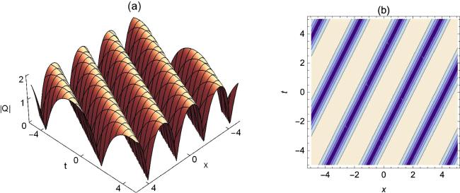
View original graphic|Download|PPT slide

Figure 1. The single-periodic wave solution of equation (3) with β₁ = 1, c = 1, a = 1 in equation (13). (a) Three dimensional plot; (b) Contour plot.

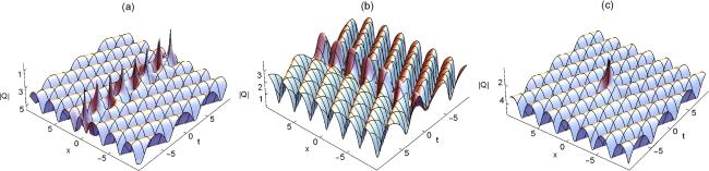
View original graphic|Download|PPT slide

Figure 2. The one-breather and first-order rogue waves on the single-periodic background of equation (3) with α = 1, $c=\sqrt{2}$, a = 1, β₃ = 1 in equation (11). (a) Akmediev breather with β₁ = 1.5, α₁ = 1.5; (b) Ma breather with β₁ = 0.7, α₁ = 0.7; (c) First-order rogue waves.

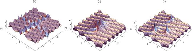
View original graphic|Download|PPT slide

Figure 3. The two-breathers and second-order rogue waves on the single-periodic background of equation (3) with α = 1, $c=\sqrt{2}$, a = 1, β₅ = 1 in equation (11). (a) Two-breathers with β₁ = 0.7, α₁ = 0.7, β₃ = 1.5, α₃ = 1.5; (b) Second-order rogue waves with S₀ = 0, S₁ = 0, S₂ = 0; (c) Second-order rogue waves with S₀ = 0, S₁ = 50, S₂ = 0.

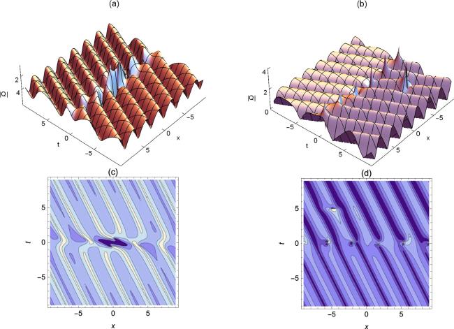
View original graphic|Download|PPT slide

Figure 4. The hybrid first-order rogue wave and one-breather solutions on the single-periodic background of equation (3) with α = 1, $c=\sqrt{2}$, a = 1, β₅ = 1, β₁ = 1, α₁ = 1 in equation (11). (a)(c) c₁ = 0, c₂ = 0; (b)(d) c₁ = 5, c₂ = −5.

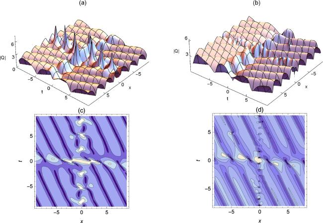
View original graphic|Download|PPT slide

Figure 5. The hybrid first-order rogue wave and two-breathers solutions on the single-periodic background of equation (3) with α = 1, $c=\sqrt{2}$, a = 1, β₇ = 1, β₃ = 0.7, α₃ = 0.7, β₅ = 1.5, α₅ = 1.5 in equation (11). (a)(c) c₁ = 0, c₂ = 0; (b)(d) c₁ = 5, c₂ = −5.

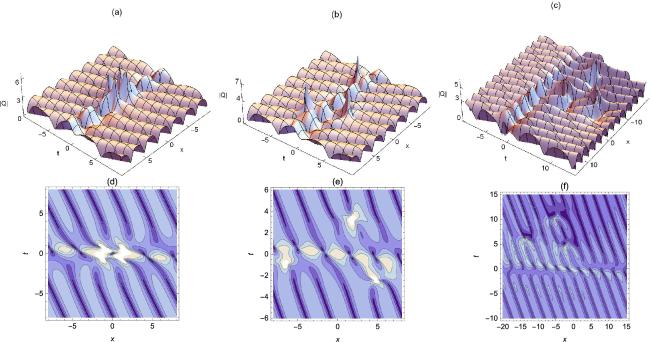
View original graphic|Download|PPT slide

Figure 6. The hybrid second-order rogue waves and one-breather solutions on the single-periodic background of equation (3) with α = 1, $c=\sqrt{2}$, a = 1, β₇ = 1, β₅ = 0, 7, α₅ = 0.7 in equation (11). (a)(d) c₁ = 0, c₂ = 0, S₀ = 0, S₁ = 0, S₂ = 0; (b)(e) c₁ = 0, c₂ = 0, S₀ = 0, S₁ = 50, S₂ = 0; (c)(f) c₁ = 5, c₂ = − 5, S₀ = 0, S₁ = 50, S₂ = 0.

5. Hybrid rogue waves and breathers solutions on the double-periodic background for the equation (3)

In this section, on the basis of solution (9), by using the Taylor expansion technology and the determinant representation of the n-transformation solution Q^[n] in section 3, the hybrid rogue waves and breather solutions on the double-periodic background for equation (3) can be constructed when n = 2k.

For n = 2k, through the combination of (5) and (10), and on the basis of the above symmetry conditions, we construct a determinant of the solution as

(12)$\begin{eqnarray}\left\{\begin{array}{l}{Q}^{[n]}=\displaystyle \frac{{{\rm{\Xi }}}_{21}^{2}}{{{\rm{\Xi }}}_{11}^{2}}Q+\displaystyle \frac{{{\rm{e}}}^{-{\rm{i}}\theta }}{\sqrt{\alpha }}\displaystyle \frac{{{\rm{\Xi }}}_{21}{{\rm{\Xi }}}_{22}}{{{\rm{\Xi }}}_{11}^{2}},\\ {R}^{[n]}=\displaystyle \frac{{{\rm{\Xi }}}_{11}^{2}}{{{\rm{\Xi }}}_{21}^{2}}R-\displaystyle \frac{{{\rm{e}}}^{{\rm{i}}\theta }}{\sqrt{\alpha }}\displaystyle \frac{{{\rm{\Xi }}}_{11}{{\rm{\Xi }}}_{12}}{{{\rm{\Xi }}}_{21}^{2}},\end{array}\right.\end{eqnarray}$

where

$\begin{eqnarray*}{{\rm{\Xi }}}_{11}=\left|\begin{array}{llllll}{\varphi }_{[1,n-\mathrm{1,1}]} & {\phi }_{[1,n-\mathrm{2,1}]} & {\varphi }_{[1,n-\mathrm{3,1}]} & \cdots & {\varphi }_{[\mathrm{1,1,1}]} & {\phi }_{[\mathrm{1,0,1}]}\\ {\varphi }_{[2,n-\mathrm{1,1}]} & {\phi }_{[2,n-\mathrm{2,1}]} & {\varphi }_{[2,n-\mathrm{3,1}]} & \cdots & {\varphi }_{[\mathrm{2,1,1}]} & {\phi }_{[\mathrm{2,0,1}]}\\ \vdots & \vdots & \vdots & \vdots & \vdots & \vdots \\ {\varphi }_{[1,n-1,l]} & {\phi }_{[1,n-2,l]} & {\varphi }_{[1,n-3,l]} & \cdots & {\varphi }_{[\mathrm{1,1},l]} & {\phi }_{[\mathrm{1,0},l]}\\ {\varphi }_{[2,n-1,l]} & {\phi }_{[2,n-2,l]} & {\varphi }_{[2,n-3,l]} & \cdots & {\varphi }_{[\mathrm{2,1},l]} & {\phi }_{[\mathrm{2,0},l]}\\ {\lambda }_{2l+1}^{n-1}{\varphi }_{2l+1} & {\lambda }_{2l+1}^{n-2}{\phi }_{2l+1} & {\lambda }_{2l+1}^{n-3}{\varphi }_{2l+1} & \cdots & {\lambda }_{2l+1}{\varphi }_{2l+1} & {\phi }_{2l+1}\\ {({\lambda }_{2l+1}^{* })}^{n-1}{\phi }_{2l+1}^{* } & {({\lambda }_{2l+1}^{* })}^{n-2}{\varphi }_{2l+1}^{* } & {({\lambda }_{2l+1}^{* })}^{n-3}{\phi }_{2l+1}^{* } & \cdots & {\lambda }_{2l+1}^{* }{\phi }_{2l+1}^{* } & {\varphi }_{2l+1}^{* }\\ \vdots & \vdots & \vdots & \vdots & \vdots & \vdots \\ {\lambda }_{2k-3}^{n-1}{\varphi }_{2k-3} & {\lambda }_{2k-3}^{n-2}{\phi }_{2k-3} & {\lambda }_{2k-3}^{n-3}{\varphi }_{2k-3} & \ldots & {\lambda }_{2k-3}{\varphi }_{2k-3} & {\phi }_{2k-3}\\ {({\lambda }_{2k-3}^{* })}^{n-1}{\phi }_{2k}^{* } & {({\lambda }_{2k-3}^{* })}^{n-2}{\varphi }_{2k}^{* } & {({\lambda }_{2k-3}^{* })}^{n-3}{\phi }_{2k-3}^{* } & \ldots & {\lambda }_{2k-3}^{* }{\phi }_{2k-3}^{* } & {\varphi }_{2k-3}^{* }\\ {\lambda }_{2k-1}^{n-1}{\varphi }_{2k-1} & {\lambda }_{2k-1}^{n-2}{\phi }_{2k-1} & {\lambda }_{2k-1}^{n-3}{\varphi }_{2k-1} & \ldots & {\lambda }_{2k-1}{\varphi }_{2k-1} & {\phi }_{2k-1}\\ {\lambda }_{2k}^{n-1}{\varphi }_{2k} & {\lambda }_{2k}^{n-2}{\phi }_{2k} & {\lambda }_{2k}^{n-3}{\varphi }_{2k} & \ldots & {\lambda }_{2k}{\varphi }_{2k} & {\phi }_{2k}\end{array}\right|\,,\end{eqnarray*}$

$\begin{eqnarray*}{{\rm{\Xi }}}_{12}=\left|\begin{array}{llllll}{\phi }_{[1,n,1]} & {\phi }_{[1,n-\mathrm{2,1}]} & {\varphi }_{[1,n-\mathrm{3,1}]} & \ldots & {\varphi }_{[\mathrm{1,1,1}]} & {\phi }_{[\mathrm{1,0,1}]}\\ {\phi }_{[2,n,1]} & {\phi }_{[2,n-\mathrm{2,1}]} & {\varphi }_{[2,n-\mathrm{3,1}]} & \ldots & {\varphi }_{[\mathrm{2,1,1}]} & {\phi }_{[\mathrm{2,0,1}]}\\ \vdots & \vdots & \vdots & \vdots & \vdots & \vdots \\ {\phi }_{[1,n,l]} & {\phi }_{[1,n-2,l]} & {\varphi }_{[1,n-3,l]} & \ldots & {\varphi }_{[\mathrm{1,1},l]} & {\phi }_{[\mathrm{1,0},l]}\\ {\phi }_{[2,n,l]} & {\phi }_{[2,n-2,l]} & {\varphi }_{[2,n-3,l]} & \ldots & {\varphi }_{[\mathrm{2,1},l]} & {\phi }_{[\mathrm{2,0},l]}\\ {\lambda }_{2l+1}^{n}{\phi }_{2l+1} & {\lambda }_{2l+1}^{n-2}{\phi }_{2l+1} & {\lambda }_{2l+1}^{n-3}{\varphi }_{2l+1} & \cdots & {\lambda }_{2l+1}{\varphi }_{2l+1} & {\phi }_{2l+1}\\ {({\lambda }_{2l+1}^{* })}^{n}{\varphi }_{2l+1}^{* } & {({\lambda }_{2l+1}^{* })}^{n-2}{\varphi }_{2l+1}^{* } & {({\lambda }_{2l+1}^{* })}^{n-3}{\phi }_{2l+1}^{* } & \cdots & {\lambda }_{2l+1}^{* }{\phi }_{2l+1}^{* } & {\varphi }_{2l+1}^{* }\\ \vdots & \vdots & \vdots & \vdots & \vdots & \vdots \\ {\lambda }_{2k-3}^{n}{\phi }_{2k-3} & {\lambda }_{2k-3}^{n-2}{\phi }_{2k-3} & {\lambda }_{2k-3}^{n-3}{\varphi }_{2k-3} & \ldots & {\lambda }_{2k-3}{\varphi }_{2k-3} & {\phi }_{2k-3}\\ {({\lambda }_{2k-3}^{* })}^{n}{\varphi }_{2k-3}^{* } & {({\lambda }_{2k-3}^{* })}^{n-2}{\varphi }_{2k-3}^{* } & {({\lambda }_{2k-3}^{* })}^{n-3}{\phi }_{2k-3}^{* } & \ldots & {\lambda }_{2k-3}^{* }{\phi }_{2k-3}^{* } & {\varphi }_{2k-3}^{* }\\ {\lambda }_{2k-1}^{n}{\phi }_{2k-1} & {\lambda }_{2k-1}^{n-2}{\phi }_{2k-1} & {\lambda }_{2k-1}^{n-3}{\varphi }_{2k-1} & \ldots & {\lambda }_{2k-1}{\varphi }_{2k-1} & {\phi }_{2k-1}\\ {\lambda }_{2k}^{n}{\phi }_{2k} & {\lambda }_{2k}^{n-2}{\phi }_{2k} & {\lambda }_{2k}^{n-3}{\varphi }_{2k} & \ldots & {\lambda }_{2k}{\varphi }_{2k} & {\phi }_{2k}\end{array}\right|\,.\end{eqnarray*}$

Here Ξ₂₁ and Ξ₂₂ are in the same form of Ξ₁₁ and Ξ₁₂ except that (φ_j; φ_j) are replaced by (φ_j; φ_j).

Through the above analysis, rogue waves can be constructed by using the first 2l lines of the above determinants. Breathers can be obtained by using lines 2l + 1 to 2k − 2 of the above determinant. Lines 2k − 1 and 2k can be used to construct a double-periodic background. Choosing different values of k, l and n in (12), we can get several types of new solutions of equation (3), including the (k − l − 1)-breathers on the double-periodic background, the lth-order rogue waves on the double-periodic background, the hybrid lth-order rogue waves and (k − l − 1)-breathers solution on the double-periodic background. By adjusting the parameters, two types of the hybrid rogue waves and breather solutions on the double-periodic background can be constructed.

The figures of the above solutions are demonstrated in figures 7–14. A more detailed discussion on the solutions will be put on section 6.

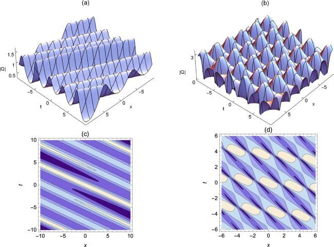
View original graphic|Download|PPT slide

Figure 7. The double-periodic wave solution of equation (3) from equation (12). (a)(c) Same direction with β₁ = 0.5, β₂ = 0.2, c = 1, a = −2. (b)(d) Different directions with ${\beta }_{1}=\sqrt{2}$, ${\beta }_{2}=\tfrac{\sqrt{2}}{2}$, $c=\sqrt{2}$, a = 1.

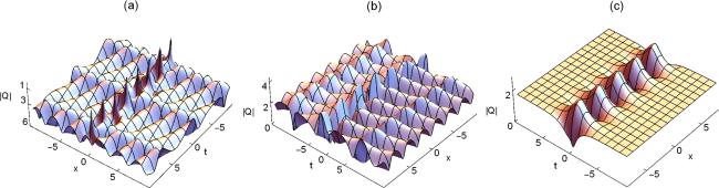
View original graphic|Download|PPT slide

Figure 8. The one-breather on the double-periodic background of equation (3) with α = 1, $c=\sqrt{2}$, a = 1 in equation (12). (a) β₃ = 1, β₄ = 0.5, β₁ = 1.5, α₁ = 1.5; (b) β₃ = 1, β₄ = 0.5, β₁ = 0.7, α₁ = 0.7; (c) β₃ = 1, β₄ = − 1, β₁ = 0.7, α₁ = 0.7.

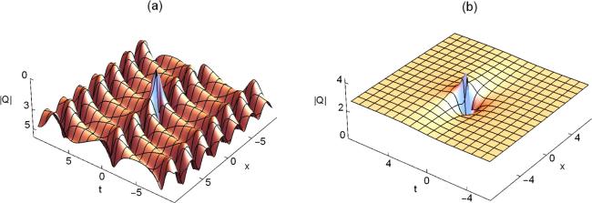
View original graphic|Download|PPT slide

Figure 9. The first-order rogue waves on the double-periodic background of equation (3) with α = 1, $c=\sqrt{2}$, a = 1 in equation (12). (a) β₃ = 1, β₄ = 0.5; (b) β₃ = 1, β₄ = −1

View original graphic|Download|PPT slide

Figure 10. The two-breathers on the double-periodic background of equation (3) with α = 1, $c=\sqrt{2}$, a = 1, α₁ = 0.7, β₁ = 0.7, α₃ = 1.5, β₃ = 1.5 in equation (12). (a) β₅ = 1, β₆ = 0.5; (b) β₅ = 1, β₆ = −1.

View original graphic|Download|PPT slide

Figure 11. The hybrid first-order rogue waves and one-breather solutions on the double-periodic background of equation (3) with α = 1, $c=\sqrt{2}$, a = 1, β₃ = 0.7, α₃ = 0.7 in equation (12). (a)(d) β₅ = 1, β₆ = 0.5, c₁ = 0, c₂ = 0; (b)(e) β₅ = 1, β₆ = 0.5, c₁ = 7, c₂ = − 7; (c)(f) β₅ = 1, β₆ = − 1, c₁ = 7, c₂ = −7.

View original graphic|Download|PPT slide

Figure 12. The second-order rogue waves on the double-periodic background of equation (3) with α = 1, $c=\sqrt{2}$,a = 1 in equation (12). (a) β₅ = 1, β₆ = 0.5, S₀ = 0, S₁ = 0, S₂ = 0; (b) β₅ = 1, β₆ = 0.5, S₀ = 0, S₁ = 50, S₂ = 0; (c) β₅ = 1, β₆ = − 1, S₀ = 0, S₁ = 50, S₂ = 0.

View original graphic|Download|PPT slide

Figure 13. The hybrid first-order rogue waves and two-breathers solutions on the double-periodic background of equation (3) with α = 1, $c=\sqrt{2}$, a = 1, β₃ = 0.7, α₃ = 0.7, β₅ = 1.5, α₅ = 1.5 in equation (12). (a)(d) c₁ = 0, c₂ = 0, β₇ = 1, β₈ = 0.5; (b)(e) c₁ = 6, c₂ = − 6, β₇ = 1, β₈ = 0.5; (c)(f) c₁ = 6, c₂ = − 6, β₇ = 1, β₈ = − 1.

View original graphic|Download|PPT slide

Figure 14. The hybrid second-order rogue waves and one-breather solutions on the double-periodic background of equation (3) with α = 1, $c=\sqrt{2}$, a = 1, β₅ = 0.7, α₅ = 0.7 in equation (12). (a)(d) c₁ = 0, c₂ = 0, S₀ = 0, S₁ = 0, S₂ = 0, β₇ = 1, β₈ = 0.5; (b)(e) c₁ = 6, c₂ = − 6, S₀ = 0, S₁ = 50, S₂ = 0, β₇ = 1, β₈ = 0.5; (c)(f) c₁ = 6, c₂ = − 6, S₀ = 0, S₁ = 50, S₂ = 0, β₇ = 1, β₈ = − 1.

6. Numerical results

In this section, by selecting different parameters, different numerical results can be obtained. By drawing their images, we perform a dynamic analysis of the obtained results, and their properties are discussed respectively.

6.1. Hybrid rogue waves and breathers solutions on the single-periodic background

	(1) For n = 1, by selecting suitable parameters, a single-periodic wave solution of equation (3) can be constructed. From (11), when n = 1, l = k = 0, we get (13)$\begin{eqnarray}Q[1]=\displaystyle \frac{{\phi }_{1}^{2}}{{\varphi }_{1}^{2}}Q+\displaystyle \frac{{{\rm{e}}}^{-{\rm{i}}(x+t)}}{\sqrt{\alpha }}\displaystyle \frac{{\lambda }_{1}{\varphi }_{1}{\phi }_{1}}{{\varphi }_{1}^{2}},\end{eqnarray}$ here we take λ₁ = β₁ and α = 1 for simplicity. Substituting (7) into (13), the following two types of solutions can be obtained depending on the choice of parameters: when $-4{c}^{2}{\lambda }_{1}^{2}+{(2+2a+{\lambda }_{1}^{2})}^{2}\gt 0$, the single-periodic wave solution of equation (3) is obtained (see figure 1). When $-4{c}^{2}{\lambda }_{1}^{2}\,+{(2+2a+{\lambda }_{1}^{2})}^{2}\lt 0$, the one-soliton solution of equation (3) can be constructed, we will not talk about it here.
	(2) For n = 3, by selecting suitable parameters, the one-breather solution on the single-periodic background and the first-order rogue waves solution on the single-periodic background of equation (3) can be constructed. Case 1 From (11), when n = 3, k = 1, l = 0, we define λ₁ = α₁ + iβ₁, λ₃ = β₃ and Im $(-4{c}^{2}{\lambda }_{1}^{2}+{(2+2a+{\lambda }_{1}^{2})}^{2})$ =0 for simplicity, the one-breather on the single-periodic background of equation (3) can be obtained. Here, we give two special classes of one-breather: when ${\alpha }_{1}^{2}={\beta }_{1}^{2}$, the Akmediev one-breather and the Ma one-breather on the single-periodic background are obtained (see figure 2(a) and (b)). Case 2 From (11), when n = 3, k = l = 1, we define ${\lambda }_{2}={\lambda }_{1}^{* }=-\sqrt{\alpha }c-{\rm{i}}\sqrt{2+2a-\alpha {c}^{2}}$ and λ₃ = β₃, the first-order rogue waves solution on the single-periodic background of equation (3) can be obtained (see figure 2(c)).
	(3) For n = 5, by selecting suitable parameters, the two-breathers solution on the single-periodic background, the second-order rogue waves solution on the single-periodic background, the hybrid first-order rogue waves and one-breather solutions on the single-periodic background of equation (3) can be constructed. Case 1 From (11), when n = 5, k = 2, l = 0, we define λ₁ = α₁ + iβ₁, λ₃ = α₃ + iβ₃, λ₅ = β₅ and Im $(-4{c}^{2}{\lambda }_{1}^{2}+{(2+2a+{\lambda }_{1}^{2})}^{2})$ = 0 for simplicity. when ${\alpha }_{1}^{2}={\beta }_{1}^{2}$, ${\alpha }_{3}^{2}={\beta }_{3}^{2}$, the two-breathers on the single-periodic background of equation (3) can be obtained, which are interactions between the Akmediev one-breather and the Ma one-breather (see figure 3(a)). Case 2 From (11), when n = 5, k = 2, l = 2, we define ${\lambda }_{2}={\lambda }_{1}^{* }=-\sqrt{\alpha }c-{\rm{i}}\sqrt{2+2a-\alpha {c}^{2}}$, ${\lambda }_{4}\,={\lambda }_{3}^{* }=-\sqrt{\alpha }c-{\rm{i}}\sqrt{2+2a-\alpha {c}^{2}}$, λ₅ = β₅. By adjusting S₀, S₁, S₂, the second-order rogue waves solution on the single-periodic background and its other shapes are obtained (see figure 3(b) and (c)). Case 3 From (11), when n = 5, k = 2, l = 1, we define λ₁ = α₁ + iβ₁, ${\lambda }_{4}={\lambda }_{3}^{* }=-\sqrt{\alpha }c-{\rm{i}}\sqrt{2+2a-\alpha {c}^{2}}$, λ₅ = β₅ and Im $(-4{c}^{2}{\lambda }_{1}^{2}+{(2+2a+{\lambda }_{1}^{2})}^{2})$ = 0 for simplicity. By adjusting the parameters, the hybrid first-order rogue waves and one-breather solution on the single-periodic background can be constructed. By adjusting the wave center parameters c₁ and c₂, we can get different shapes of the solution (see figure 4).
	(4) For n = 7, by selecting suitable parameters, the three-breather solutions on the single-periodic background, the third-order rogue waves solution on the single-periodic background, the hybrid first-order rogue waves and two-breathers solution, and the hybrid second-order rogue waves and one-breather solution on the single-periodic background of equation (3) can be constructed. Case 1 From (11), when n = 7, k = 3, l = 0, we define λ₁ = α₁ + iβ₁, λ₃ = α₃ + iβ₃, λ₅ = α₅ + iβ₅, λ₇ = β₇ and Im $(-4{c}^{2}{\lambda }_{1}^{2}+{(2+2a+{\lambda }_{1}^{2})}^{2})$ = 0 for simplicity. By adjusting parameters, the three-breathers on the single-periodic background of equation (3) can be obtained, of which we will not go into detail here. Case 2 From (11), when n = 7, k = 3, l = 1, we define ${\lambda }_{2}={\lambda }_{1}^{* }=-\sqrt{\alpha }c-{\rm{i}}\sqrt{2+2a-\alpha {c}^{2}}$, λ₃ =α₃ + iβ₃, λ₅ = α₅ + iβ₅, λ₇ = β₇ and Im $(-4{c}^{2}{\lambda }_{1}^{2}\,+{(2+2a+{\lambda }_{1}^{2})}^{2})$ = 0 for simplicity. By adjusting the parameters, the hybrid first-order rogue waves and two-breathers solutions on the single-periodic background can be constructed. By adjusting the wave center parameters c₁ and c₂, we can get different shapes of the solution (see figure 5). Case 3 From (11), when n = 7, k = 3, l = 2, we define ${\lambda }_{2}={\lambda }_{1}^{* }=-\sqrt{\alpha }c-{\rm{i}}\sqrt{2+2a-\alpha {c}^{2}}$, ${\lambda }_{4}={\lambda }_{3}^{* }=-\sqrt{\alpha }c-{\rm{i}}\sqrt{2+2a-\alpha {c}^{2}}$, λ₅ = α₅ + iβ₅, λ₇ = β₇ and Im $(-4{c}^{2}{\lambda }_{1}^{2}+{(2+2a+{\lambda }_{1}^{2})}^{2})$ = 0 for simplicity. The hybrid second-order rogue waves and one-breather solutions on the single-periodic background can be constructed. By adjusting S₀, S₁, S₂, the wave center parameters c₁ and c₂, we can get different shapes of the solution (see figure 6). Case 4 From (11), when n = 7, k = l = 3, we define ${\lambda }_{2}={\lambda }_{1}^{* }=-\sqrt{\alpha }c-{\rm{i}}\sqrt{2+2a-\alpha {c}^{2}}$, ${\lambda }_{4}={\lambda }_{3}^{* }=-\sqrt{\alpha }c-{\rm{i}}\sqrt{2+2a-\alpha {c}^{2}}$, ${\lambda }_{6}={\lambda }_{5}^{* }=-\sqrt{\alpha }c-{\rm{i}}\sqrt{2+2a-\alpha {c}^{2}}$, λ₇ = β₇. The third-order rogue waves on the single-periodic background can be constructed. By adjusting S₀, S₁, S₂, the wave center parameters c₁ and c₂, we can get different shapes of the solution, of which we will not go into details here.

Based on the above analysis, it is easy to observe that when n = 2k + 1, l = 0, the k-breathers on the single-periodic background can be obtained. When n = 2k + 1, l = k, the kth-order rogue waves on the single-periodic background can be obtained. Similarly, the hybrid solution can be generalized to nth-order: when n = 2k + 1, l = k − s, the hybrid k − s th-order rogue waves and s-breathers solutions on the single-periodic background can be constructed. We see that the the above solutions propagate stably on the single-periodic background with periodic patterns, without interference from the background. The forms of the breathers on the single-periodic background and the rogue waves on the single-periodic background are the same as [37, 48]. The forms of the hybrid rogue waves and breather solutions on the single-periodic background are the same as [40, 41].

6.2. Hybrid rogue waves and breathers solutions on the double-periodic background

(1) For n = 2, by selecting suitable parameters, a double-periodic wave solution of equation (3) can be constructed.

From (12), when n = 2, k = 1, l = 0, we define λ₁ = β₁, λ₂ = β₂ and β₂ ≠ ± β₁. A double-periodic wave solution can be obtained. Here, we give two types of double-periodic wave solution according to their different propagation directions (see figure 7). It is clear that the collision of double-periodic wave solutions is elastic. When λ₁ = α₁ + iβ₁, one-breather can be obtained. The shape of the solution is similar to figure 8(c), we will not go into detail here.

(2) For n = 4, by selecting suitable parameters, the one-breather on the double-periodic background and the first-order rogue waves on the double-periodic background of equation (3) can be constructed.

Case 1 From (12), when n = 4, k = 2, l = 0, we define λ₁ = α₁ + iβ₁, λ₃ = β₃, λ₄ = β₄ and Im $(-4{c}^{2}{\lambda }_{1}^{2}+{(2+2a+{\lambda }_{1}^{2})}^{2})$ = 0 for simplicity. By adjusting the parameters, the one-breather on the double-periodic background can be constructed (see figure 8(a) and (b)). In particular, when β₄ = − β₃, a plane wave background will appear (see figure 8(c)). Apart from the above, taking λ₃ = α₃ + iβ₃, the two-breathers on the plane wave background can be obtained. The shape of the solution is similar to figure 10(b), and we will not go into detail here.

Case 2 From (12), when n = 4, k = 2, l = 1, we define ${\lambda }_{2}={\lambda }_{1}^{* }=-\sqrt{\alpha }c-{\rm{i}}\sqrt{2+2a-\alpha {c}^{2}}$, λ₃ = β₃, λ₄ = β₄. By adjusting the parameters, the first-order rogue waves on the double-periodic background can be constructed (see figure 9(a)). In particular, when β₄ = − β₃, the first-order rogue waves on the double-periodic background will degenerate to the first-order rogue waves on the plane wave background (see figure 9(b)). Apart from the above, taking λ₃ = α₃ +iβ₃ and Im $(-4{c}^{2}{\lambda }_{1}^{2}+{(2+2a+{\lambda }_{1}^{2})}^{2})$ = 0 for simplicity, the hybrid first-order rogue waves and one-breather on the plane wave background can be obtained. The shape of the solution is similar to figure 11(c), and we will not go into detail here.

(3) For n = 6, by selecting suitable parameters, the two-breathers on the double-periodic background, the second-order rogue waves on the double-periodic background, and the hybrid first-order rogue waves and one-breather on the double-periodic background of equation (3) can be constructed.

Case 1 From (12), when n = 6, k = 3, l = 0, we define λ₁ = α₁ + iβ₁, λ₃ = α₃ + iβ₃, λ₅ = β₅, λ₆ = β₆ and Im $(-4{c}^{2}{\lambda }_{1}^{2}+{(2+2a+{\lambda }_{1}^{2})}^{2})$ = 0 for simplicity. By adjusting the parameters, the two-breathers on the double-periodic background can be constructed (see figure 10(a)). In particular, when β₄ = − β₃, a plane wave background will appear (see figure 10(b)). Apart from the above, taking λ₅ = α₅ + iβ₅, the three-breathers on the plane wave background can be obtained and we will not go into detail here.

Case 2 From (12), when n = 6, k = 3, l = 1, we define ${\lambda }_{2}={\lambda }_{1}^{* }=-\sqrt{\alpha }c-{\rm{i}}\sqrt{2+2a-\alpha {c}^{2}}$, λ₃ =α₃ + iβ₃, λ₅ = β₅, λ₆ = β₆ and Im $(-4{c}^{2}{\lambda }_{1}^{2}\,+{(2+2a+{\lambda }_{1}^{2})}^{2})$ = 0 for simplicity. The hybrid first-order rogue waves and one-breather on the double-periodic background of equation (3) can be constructed (see figure 11(a)). By adjusting the wave center parameters c₁ and c₂, we can get different shapes of the solution (see figure 11(b)). In particular, when β₆ = − β₅, the hybrid first-order rogue waves and one-breather on the double-periodic background will degenerate to the hybrid first-order rogue waves and one-breather on the plane wave background (see figure 11(c)). Apart from the above, taking λ₅ = α₅ + iβ₅, the hybrid first-order rogue waves and two-breathers on the plane wave background can be obtained. The shape of the solution is similar to figure 13(c), and we will not go into detail here.

Case 3 From (12), when n = 6, k = 3, l = 2, we define ${\lambda }_{2}={\lambda }_{1}^{* }=-\sqrt{\alpha }c-{\rm{i}}\sqrt{2+2a-\alpha {c}^{2}}$, ${\lambda }_{4}\,={\lambda }_{3}^{* }=-\sqrt{\alpha }c-{\rm{i}}\sqrt{2+2a-\alpha {c}^{2}}$, λ₅ = β₅, λ₆ = β₆. By adjusting the parameters, the second-order rogue waves on the double-periodic background of equation (3) can be constructed (see figure 12(a)). By adjusting S₀, S₁ and S₂, we can get different shapes of the solution (see figure 12(b)). When β₆ = − β₅, a plane wave background will appear (see figure 12(c)). Apart from the above, taking λ₅ = α₅ + iβ₅, the hybrid second-order rogue waves and one-breather on the plane wave background can be obtained. The shape of the solution is similar to figure 14(c), and we will not go into detail here.

(3) For n = 8, by selecting suitable parameters, the three-breathers on the double-periodic background, the third-order rogue waves on the double-periodic background, the hybrid first-order rogue waves and two-breathers on the double-periodic background, and the hybrid second-order rogue waves and one-breather on the double-periodic background of equation (3) can be constructed.

Case 1 From (12), when n = 8, k = 4, l = 0, we define λ₁ = α₁ + iβ₁, λ₃ = α₃ + iβ₃, λ₅ = α₅ + iβ₅, λ₇ = β₇, λ₈ = β₈ and Im $(-4{c}^{2}{\lambda }_{1}^{2}+{(2+2a+{\lambda }_{1}^{2})}^{2})$ = 0 for simplicity. By adjusting the parameters, the three-breathers on the double-periodic background can be constructed. Apart from the above, taking λ₇ = α₇ + iβ₇, the four-breathers on the plane wave background can be obtained and we will not go into detail here.

Case 2 From (12), when n = 8, k = 4, l = 1, we define ${\lambda }_{2}={\lambda }_{1}^{* }=-\sqrt{\alpha }c-{\rm{i}}\sqrt{2+2a-\alpha {c}^{2}}$, λ₃ = α₃ + iβ₃, λ₅ = α₅ + iβ₅, λ₇ = β₇, λ₈ = β₈ and Im $(-4{c}^{2}{\lambda }_{1}^{2}\,+{(2+2a+{\lambda }_{1}^{2})}^{2})$ = 0 for simplicity. The hybrid first-order rogue waves and two-breathers on the double-periodic background of equation (3) can be constructed (see figure 13(a)). By adjusting the wave center parameters c₁ and c₂, we can get different shapes of the solution (see figure 13(b)). When β₈ = − β₇, the hybrid first-order rogue waves and two-breathers on the double-periodic background will degenerate to the hybrid first-order rogue waves and two-breathers on the plane wave background (see figure 13(c)). Apart from the above, taking λ₇ = α₇ + iβ₇, the hybrid first-order rogue waves and three-breathers on the plane wave background can be obtained, and we will not go into detail here.

Case 3 From (12), when n = 8, k = 4, l = 2, we define ${\lambda }_{2}={\lambda }_{1}^{* }=-\sqrt{\alpha }c-{\rm{i}}\sqrt{2+2a-\alpha {c}^{2}}$, ${\lambda }_{4}={\lambda }_{3}^{* }=-\sqrt{\alpha }c-{\rm{i}}\sqrt{2+2a-\alpha {c}^{2}}$, ${\lambda }_{6}={\lambda }_{5}^{* }={\alpha }_{5}-{\rm{i}}{\beta }_{5}$, λ₇ = β₇, λ₈ = β₈ and Im $(-4{c}^{2}{\lambda }_{1}^{2}+{(2+2a+{\lambda }_{1}^{2})}^{2})$ = 0 for simplicity. The hybrid second-order rogue waves and one-breather on the double-periodic background of equation (3) can be constructed (see figure 14(a)). By adjusting S₀, S₁, S₂, the wave center parameters c₁ and c₂, we can get different shapes of the solution (see figure 14(b)). When β₈ = − β₇, the hybrid second-order rogue waves and one-breather on the double-periodic background will degenerate to the hybrid second-order rogue waves and one-breather on the plane wave background (see figure 14(c)). Apart from the above, taking λ₇ = α₇ + iβ₇, the hybrid second-order rogue waves and two-breathers on the plane wave background can be obtained, and we will not go into detail here.

Case 4 From (12), when n = 8, k = 4, l = 3, we define ${\lambda }_{2}={\lambda }_{1}^{* }=-\sqrt{\alpha }c-{\rm{i}}\sqrt{2+2a-\alpha {c}^{2}}$, ${\lambda }_{4}={\lambda }_{3}^{* }\,=-\sqrt{\alpha }c-{\rm{i}}\sqrt{2+2a-\alpha {c}^{2}}$, ${\lambda }_{6}={\lambda }_{5}^{* }=-\sqrt{\alpha }c-{\rm{i}}\sqrt{2+2a-\alpha {c}^{2}}$, λ₇ = β₇, λ₈ = β₈. The third-order rogue waves on the double-periodic background of equation (3) can be constructed. By adjusting S₀, S₁, S₂, we can get different shapes of the solution. Apart from the above, taking λ₇ = α₇ + iβ₇, the hybrid third-order rogue waves and one-breather on the plane wave background can be obtained, and we will not go into detail here.

Based on the above analysis, we define λ_2k = β_2k and λ_2k−1 = β_2k−1 when n = 2k. It is easy to observe that when l = 0, the k − 1-breathers on the double-periodic background can be obtained. When l = k − 1, the k − 1 th-order rogue waves on the double-periodic background can be obtained. Similarly, the hybrid solution can be generalized to nth-order: when l = k − s (1 < s < k), the hybrid k − s th-order rogue waves and s − 1-breathers solutions on the double-periodic background can be constructed. Apart from the above, taking ${\lambda }_{2k}={\lambda }_{2k-1}^{* }={\alpha }_{2k-1}-{\rm{i}}{\beta }_{2k-1}$, it is easy to observe that when l = 0, the k-breathers on the plane wave background can be obtained. When l = k, the kth-order rogue waves on the plane wave background can be obtained. When l = k − s (0 < s < k), the hybrid k − s th-order rogue waves and s-breathers solutions on the plane wave background can be constructed. Obviously, the double-periodic background cannot change the amplitude or propagation direction of the solutions. When β_2k = − β_2k−1, a plane wave background will appear, which is because the periodic backgrounds with the same period but opposite directions just offset each other. The forms of the breathers on the double-periodic background and the rogue waves on the double-periodic background are the same as [38, 48].

7. Conclusion

In summary, by constructing a new determinant of the n-fold DT, the hybrid breathers and rogue waves solutions can be constructed on the different background. Through the odd-fold DT, the hybrid breathers and rogue wave solutions on the single-periodic background will be obtained. Through the even-fold DT, the hybrid breathers and rogue wave solutions on the double-periodic or the plane wave background are obtained. By adjusting S₀, S₁, S₂, the wave center parameters c₁ and c₂, different shapes of the hybrid solutions are obtained. In the process of constructing the solutions, we find that the single- or the double-periodic background do not affect the propagation direction of the solutions. We hope that the construction of hybrid solutions on the double-periodic background can help readers analyze some complex physical systems. On this basis, additional types of the hybrid solutions can be constructed through this method in the future.

Competing interests

The authors declare that there is no conflict of interest.

Authors contributions

DZ J conceived and wrote the manuscript. Zhaqilao revised the manuscript. All authors discussed the results and commented on the manuscript.

This work is supported by the National Natural Science Foundation of China under (Grant No. 12361052), the Natural Science Foundation of Inner Mongolia Autonomous Region, China under (Grant No. 2020LH01010, 2022ZD05), Program for Innovative Research Team in Universities of Inner Mongolia Autonomous Region (Grant No. NMGIRT2414) and the Fundamental Research Founds for the Inner Mongolia Normal University (Grant No. 2022JBTD007).

References

Publishing order | Descend order by publishing year | Descend order by cited within

1	Baleanu D, Alshomrani A S, Ullah M Z 2021 A new fourth-order integrable nonlinear equation: Breather, rogue wave, other lump interaction phenomena, and conservation laws Adv. Differ. Equ. 2021 1 16 DOI

2	Wang L H, Porsezian K, He J S 2013 Breather and rouge wave solutions of a generalized nonlinear Schrödinger equation Phys. Rev. E 87 053202 DOI

3	Zhao H Q, Yuan J Y, Zhu Z N 2018 Integrable semi-discrete Kundu-Eckhaus equation: Darboux transformation, breather, rogue wave and continuous limit theory J. Nonlinear Sci. 28 43 68 DOI

4	Zhaqilao 2013 Rogue waves and rational solutions of a (3+ 1)-dimensional nonlinear evolution equation Phys. Lett. A 377 3021 3026 DOI

5	Zhaqilao 2017 The interaction solitons for the complex short pulse equation Commun. Nonlinear Sci. Numer. Simul. 47 379 393 DOI

6	Noja D 2014 Nonlinear Schrödinger equation on graphs: recent results and open problems Phil. Trans. R. Soc. A. 372 20130002 DOI

7	Tang Y, He C, Zhou M 2018 Darboux transformation of a new generalized nonlinear Schrödinger equation: soliton solutions, breather solutions, and rogue wave solutions Nonlinear Dyn. 92 2023 2036 DOI

8	Liu C, Chen S C, Akhmediev N 2024 Fundamental and Second-Order Superregular Breathers in Vector Fields Phys. Rev. Lett. 132 027201 DOI

9	Chen S C, Liu C, Akhmediev N 2023 Higher-order modulation instability and multi- Akhmediev breathers of Manakov equations: Frequency jumps over the stable gaps between the instability bands Phys. Rev. A 107 063507 DOI

10	Liu C, Chen S C, Yao X 2022 Modulation instability and non-degenerate Akhmediev breathers of Manakov equations Chin. Phys. Lett. 39 094201 DOI

11	Che W J, Chen S C, Liu C 2022 Nondegenerate Kuznetsov-Ma solitons of Manakov equations and their physical spectra Phys. Rev. A 105 043526 DOI

12	Liu C, Chen S C, Yao X 2022 Non-degenerate multi-rogue waves and easy ways of their excitation Physica D 433 133192 DOI

13	Che W J, Liu C, Akhmediev N 2023 Fundamental and second-order dark soliton solutions of two-and three-component Manakov equations in the defocusing regime Phys. Rev. E 107 054206 DOI

14	Bludov Y V, Konotop V V, Akhmediev N 2009 Matter rogue waves Phys. Rev. A 80 033610 DOI

15	Akhmedievt N, Ankiewicz A, Taki M 2009 Waves that appear from nowhere and disappear without a trace Phys. Lett. A 373 675 678 DOI

16	Grammaticos B, Kosmann-Schwarzbach Y, Tamizhmani K M 2004 Integrability of nonlinear systems Berlin Springer DOI

17	Bluman G W, Kumei S 1989 Symmetries and differential equations Berlin Springer DOI

18	Zhang Y, Cheng Y, He J 2017 Riemann-Hilbert method and N-soliton for two-component Gerdjikov-Ivanov equation J. Nonlinear Math. Phys. 24 210 223

19	Zhaqilao, Sirendaoreji 2010 N-Soliton solutions of the KdV6 and mKdV6 equations J. Math. Phys. 51 073516 DOI

20	Zhaqilao, Qiao Z J 2011 Darboux transformation and explicit solutions for two integrable equations Math. Anal. Appl. 380 794 806 DOI

21	Xu S, He J, Wang L 2011 The Darboux transformation of the derivative nonlinear Schrödinger equation J. Phys. A: Math. Theor. 44 305203 DOI

22	Ma Y L, Li B Q 2022 Hybrid rogue wave and breather solutions for a complex mKdV equation in few-cycle ultra-short pulse optics Eur. Phys. J. Plus. 137 1 10 DOI

23	Kumar S, Mohan B, Kumar R 2022 Lump, soliton, and interaction solutions to a generalized two-mode higher-order nonlinear evolution equation in plasma physics Nonlinear Dyn. 110 693 704 DOI

24	Ma W X 2018 Dynamics of mixed lump-solitary waves of an extended (2+1)-dimensional shallow water wave model Phys. Lett. A 382 3262 3268 DOI

25	Wen X Y, Yan Z 2017 Higher-order rational solitons and rogue-like wave solutions of the (2+1)-dimensional nonlinear fluid mechanics equations Commun. Nonlinear Sci. Numer. Simul. 43 311 329 DOI

26	Zhao D, Zhaqilao 2021 On the role of K+ L+ M-wave mixing effect in the (2+1)-dimensional KP I equation Eur. Phys. J. Plus. 136 399 DOI

27	Zhao D, Zhaqilao 2020 Three-wave interactions in a more general (2+1)-dimensional Boussinesq equation Eur. Phys. J. Plus. 135 1 16 DOI

28	Shi W, Zhaqilao 2023 Higher-order mixed solution and breather solution on a periodic background for the Kundu equation Commun. Nonlinear Sci. Numer. Simul. 119 107134 DOI

29	Du Z, Guo C M, Guo Q 2022 Hybrid structures of rogue waves and breathers for the coupled Hirota system with negative coherent coupling Phys. Scripta. 97 075205 DOI

30	Li B Q 2022 Hybrid breather and rogue wave solution for a (2+1)-dimensional ferromagnetic spin chain system with variable coefficients Int. J. Comput. Math. 97 506 519 DOI

31	Li B Q, Ma Y L 2020 Extended generalized Darboux transformation to hybrid rogue wave and breather solutions for a nonlinear Schrödinger equation Appl. Math. Comput. 386 125469 DOI

32	Wen X Y, Lin Z 2022 Modulational instability and position controllable discrete rogue waves with interaction phenomena in the semi-discrete complex coupled dispersionless system Wave Motion. 112 102932 DOI

33	Solli D R, Ropers C, Jalali B 2008 Active control of rogue waves for stimulated supercontinuum generation Phys. Rev. Lett. 101 233902 DOI

34	Chen F, Zhang H Q 2021 Rogue waves on the periodic background in the higher-order modified Korteweg-de Vries equation Mod. Phys. Lett. B 35 2150081 DOI

35	Wang Z J, Zhaqilao 2022 Rogue wave solutions for the generalized fifth-order nonlinear Schrödinger equation on the periodic background Wave Motion 108 102839 DOI

36	Peng W Q, Pu J C, Chen Y 2022 PINN deep learning method for the Chen-Lee-Liu equation: Rogue wave on the periodic background Commun. Nonlinear Sci. Numer. Simul. 105 106067 DOI

37	Ding C C, Gao Y T, Li L Q 2019 Breathers and rogue waves on the periodic background for the Gerdjikov-Ivanov equation for the Alfvén waves in an astrophysical plasma Chaos Solitons Fractals. 120 259 265 DOI

38	Chen J, Pelinovsky D E, White R E 2019 Rogue waves on the double-periodic background in the focusing nonlinear Schrödinger equation Phys. Rev. E 100 052219 DOI

39	Kedziora D J, Ankiewicz A, Akhmediev N 2014 Rogue waves and solitons on a cnoidal background Eur. Phys. J. Spec. Top. 223 43 62 DOI

40	Xue B, Shen J, Geng X G 2020 Breathers and breather-rogue waves on a periodic background for the derivative nonlinear Schrödinger equation Phys. Scr. 95 055216 DOI

41	Yang H, Guo R 2023 A study of periodic solutions and periodic background solutions for the reverse-space-time modified nonlinear Schrödinger equation Wave Motion 117 103112 DOI

42	Kaup D J, Newell A C 1978 An exact solution for a derivative nonlinear Schrödinger equation J. Math. Phys. 19 798 801 DOI

43	Liu C, Akhmediev N 2019 Super-regular breathers in nonlinear systems with self-steepening effect Phys. Rev. E 100 062201 DOI

44	Liu C, Wu Y H, Chen S C 2021 Exact analytic spectra of asymmetric modulation instability in systems with self-steepening effect Phys. Rev. Lett. 127 094102 DOI

45	Kundu A 2006 Integrable hierarchy of higher nonlinear schrödinger type equations Symmetry Integr. Geom. 2 78 DOI

46	Kundu A 1984 Landau-Lifshitz and higher-order nonlinear systems gauge generated from nonlinear schrödinger type equations J. Math. Phys. 25 3433 DOI

47	Xu S, He J, Wang L 2011 The Darboux transformation of the derivative nonlinear Schrödinger equation Phys. A: Math. Theor. 44 305203 DOI

48	Zhou H, Chen Y 2021 Breathers and rogue waves on the double-periodic background for the reverse-space-time derivative nonlinear Schrödinger equation Nonlinear Dyn. 106 3437 3451 DOI

49	Shan S, Li C, He J 2013 On rogue wave in the Kundu-DNLS equation Commun. Nonlinear Sci. Numer. Simul. 18 3337 3349 DOI

50	Fan E 2001 A Liouville integrable Hamiltonian system associated with a generalized Kaup-Newell spectral problem Physica A 301 105 113 DOI

51	Fan E 2001 Integrable systems of derivative nonlinear Schrödinger type and their multi-Hamiltonian structure Phys. A: Math. Theor. 34 513 DOI

Options

Outlines

模态框（Modal）标题

Abstract

Cite this article

1. Introduction

2. Lax pair and n-transformed solutions of the equation (3)

3. Mathematical method

4. Hybrid rogue waves and breathers solution on the single-periodic background for the equation (3)

Figure 1. The single-periodic wave solution of equation (3) with β1 = 1, c = 1, a = 1 in equation (13). (a) Three dimensional plot; (b) Contour plot.

Figure 2. The one-breather and first-order rogue waves on the single-periodic background of equation (3) with α = 1, $c=\sqrt{2}$, a = 1, β3 = 1 in equation (11). (a) Akmediev breather with β1 = 1.5, α1 = 1.5; (b) Ma breather with β1 = 0.7, α1 = 0.7; (c) First-order rogue waves.

Figure 4. The hybrid first-order rogue wave and one-breather solutions on the single-periodic background of equation (3) with α = 1, $c=\sqrt{2}$, a = 1, β5 = 1, β1 = 1, α1 = 1 in equation (11). (a)(c) c1 = 0, c2 = 0; (b)(d) c1 = 5, c2 = −5.

Figure 5. The hybrid first-order rogue wave and two-breathers solutions on the single-periodic background of equation (3) with α = 1, $c=\sqrt{2}$, a = 1, β7 = 1, β3 = 0.7, α3 = 0.7, β5 = 1.5, α5 = 1.5 in equation (11). (a)(c) c1 = 0, c2 = 0; (b)(d) c1 = 5, c2 = −5.

5. Hybrid rogue waves and breathers solutions on the double-periodic background for the equation (3)

Figure 7. The double-periodic wave solution of equation (3) from equation (12). (a)(c) Same direction with β1 = 0.5, β2 = 0.2, c = 1, a = −2. (b)(d) Different directions with ${\beta }_{1}=\sqrt{2}$, ${\beta }_{2}=\tfrac{\sqrt{2}}{2}$, $c=\sqrt{2}$, a = 1.

Figure 8. The one-breather on the double-periodic background of equation (3) with α = 1, $c=\sqrt{2}$, a = 1 in equation (12). (a) β3 = 1, β4 = 0.5, β1 = 1.5, α1 = 1.5; (b) β3 = 1, β4 = 0.5, β1 = 0.7, α1 = 0.7; (c) β3 = 1, β4 = − 1, β1 = 0.7, α1 = 0.7.

Figure 9. The first-order rogue waves on the double-periodic background of equation (3) with α = 1, $c=\sqrt{2}$, a = 1 in equation (12). (a) β3 = 1, β4 = 0.5; (b) β3 = 1, β4 = −1

Figure 10. The two-breathers on the double-periodic background of equation (3) with α = 1, $c=\sqrt{2}$, a = 1, α1 = 0.7, β1 = 0.7, α3 = 1.5, β3 = 1.5 in equation (12). (a) β5 = 1, β6 = 0.5; (b) β5 = 1, β6 = −1.

Figure 12. The second-order rogue waves on the double-periodic background of equation (3) with α = 1, $c=\sqrt{2}$,a = 1 in equation (12). (a) β5 = 1, β6 = 0.5, S0 = 0, S1 = 0, S2 = 0; (b) β5 = 1, β6 = 0.5, S0 = 0, S1 = 50, S2 = 0; (c) β5 = 1, β6 = − 1, S0 = 0, S1 = 50, S2 = 0.

6. Numerical results

6.1. Hybrid rogue waves and breathers solutions on the single-periodic background

6.2. Hybrid rogue waves and breathers solutions on the double-periodic background

7. Conclusion

Competing interests

Authors contributions

References

Figure 1. The single-periodic wave solution of equation (3) with β₁ = 1, c = 1, a = 1 in equation (13). (a) Three dimensional plot; (b) Contour plot.

Figure 2. The one-breather and first-order rogue waves on the single-periodic background of equation (3) with α = 1, $c=\sqrt{2}$, a = 1, β₃ = 1 in equation (11). (a) Akmediev breather with β₁ = 1.5, α₁ = 1.5; (b) Ma breather with β₁ = 0.7, α₁ = 0.7; (c) First-order rogue waves.

Figure 4. The hybrid first-order rogue wave and one-breather solutions on the single-periodic background of equation (3) with α = 1, $c=\sqrt{2}$, a = 1, β₅ = 1, β₁ = 1, α₁ = 1 in equation (11). (a)(c) c₁ = 0, c₂ = 0; (b)(d) c₁ = 5, c₂ = −5.

Figure 5. The hybrid first-order rogue wave and two-breathers solutions on the single-periodic background of equation (3) with α = 1, $c=\sqrt{2}$, a = 1, β₇ = 1, β₃ = 0.7, α₃ = 0.7, β₅ = 1.5, α₅ = 1.5 in equation (11). (a)(c) c₁ = 0, c₂ = 0; (b)(d) c₁ = 5, c₂ = −5.

Figure 7. The double-periodic wave solution of equation (3) from equation (12). (a)(c) Same direction with β₁ = 0.5, β₂ = 0.2, c = 1, a = −2. (b)(d) Different directions with ${\beta }_{1}=\sqrt{2}$, ${\beta }_{2}=\tfrac{\sqrt{2}}{2}$, $c=\sqrt{2}$, a = 1.

Figure 8. The one-breather on the double-periodic background of equation (3) with α = 1, $c=\sqrt{2}$, a = 1 in equation (12). (a) β₃ = 1, β₄ = 0.5, β₁ = 1.5, α₁ = 1.5; (b) β₃ = 1, β₄ = 0.5, β₁ = 0.7, α₁ = 0.7; (c) β₃ = 1, β₄ = − 1, β₁ = 0.7, α₁ = 0.7.

Figure 9. The first-order rogue waves on the double-periodic background of equation (3) with α = 1, $c=\sqrt{2}$, a = 1 in equation (12). (a) β₃ = 1, β₄ = 0.5; (b) β₃ = 1, β₄ = −1

Figure 10. The two-breathers on the double-periodic background of equation (3) with α = 1, $c=\sqrt{2}$, a = 1, α₁ = 0.7, β₁ = 0.7, α₃ = 1.5, β₃ = 1.5 in equation (12). (a) β₅ = 1, β₆ = 0.5; (b) β₅ = 1, β₆ = −1.