


1. Introduction
Some new phenomena that do not exist in linear systems can appear in nonlinear issues. So, the main reason to study nonlinear problems is to understand these new system properties and make linear methods more accurate [1]. Hence, it is recommended that thorough research be conducted on solutions for nonlinear issues and that alternatives that resemble a well-established linear solution be explored. This is how perturbation methods are used to solve various nonlinear problems [2]. Some of the movements in nature that have the property of repeating themselves at regular intervals of time are called periodic. In these movements, a particle moves between two extreme positions. Therefore, the movement occurs in repetitive cycles, each of which are the same. Examples of this type of movement ranges from the strings on a guitar to the vibrations of atoms in a solid. Periodic movements are oscillations where physical quantities fluctuate around a balance value. Among the oscillatory movements, we have a suspended mass of a vertical spring, whose motion can be described as a single coordinate of distance with the up and down movement [3]. There are many types of oscillatory movements [4–7], some of which are highly complex. However, a very frequently encountered form is also straightforward: simple harmonic motion. An object moves in a simple harmonic way when the resultant force acting on it is in the opposite direction and directly proportional to its displacement. The initial state is characterized by an equilibrium condition in which the net force is balanced and equal to zero. In recent times, there has been a surge in the scholarly community’s attention towards the investigation and discourse surrounding the mathematical pendulum, as observed among mathematicians and physicists. This particular system is widely regarded as a fundamental model for investigating nonlinear dynamics and intricate phenomena across diverse domains of scientific inquiry and practical applications, such as electrical circuits [8] and the phenomenon of charge density waves [9].
In beginning science and math courses, the pendulum equation is commonly presented as a nonlinear ordinary differential equation (ODE) that is physically meaningful. It is worth noting that the general solution of this equation cannot be represented using elementary functions. The ODE acts as a tool to stimulate phase plane and stability analyses. Linearizing the equation to consider minor deviations enables a classical harmonic oscillator solution to emerge. For almost a century, it has been established that the Jacobi elliptic functions can provide the analytical solution for the pendulum equation, wherein an angle is stated as a function of time [1, 2]. As far as we know, many techniques have been devoted to analyzing different types of nonlinear oscillators [10–14]. Different numerical and analytical methods have successfully been used to study other dynamic systems. For example, the modified homotopy perturbation method (HPM) was used to examine the delayed third-order damped Duffing oscillator [15]. Also, the third-order fractional Van der Pol–Duffing oscillator has been analyzed using a new non-perturbative approach [16]. The HPM was applied for analyzing both fractal space Duffing oscillators with arbitrary initial conditions [17] and a generalized Duffing oscillator [18]. Furthermore, He and his group [19–22] proposed specific alterations to the HPM for analyzing the dynamics of highly nonlinear evolution equations. These adjustments offer improved efficiency and significantly enhanced approximation accuracy compared to the conventional HMP. Therefore, these improvements to the HPM allow for accurately analyzing many evolution/wave/motion equations to ensure a high level of matching between the theoretical results and laboratory results or observations described by the equations under study. Moreover, the frequency prediction method has successfully evaluated numerous nonlinear oscillators, including singular oscillators, tangent oscillators, hyperbolic tangent oscillators, and microelectromechanical system oscillators, regardless of their initial conditions [23]. He’s HPM was employed to find the analytical approximation of a rotating Pendulum System oscillator [24]. Also, the authors [24] compared the obtained analytical approximation with the Rung–Kutta (RK4) numerical approximation. The Multiple Scales Method (MSM) and Krýlov–Bogoliúbov–Mitropólsky method (KBMM) were employed to provide approximate solutions for a time Delay Duffing–Helmholtz equation [25]. Furthermore, both KBMM and MSM were used for analyzing and solving several nonlinear oscillators with strong nonlinearity [26–32].
This study examines a generalized pendulum system called a generalized rotating pendulum oscillator [33, 34]. The objective is to derive analytical approximations using the MSM. The system under consideration is a linear pendulum in which a string does not suspend the bob, as this may become loose. Alternatively, the bob is upheld by a slender and inflexible rod hinged to facilitate rotation. This rotation occurs along a vertical axis, with the bob moving at a specific angular velocity referred to as ‘ω’ and positioned at a distance of ‘r’. This configuration can be depicted as bearing a resemblance to the gondola of a roundabout. The plane of oscillation is defined by the vertical axis and the ‘gallows’ structure, as seen in figure 1. Within this theoretical framework; the gondola is subject to the influence of two distinct forces that exert their effects throughout its designated trajectory, known as the centrifugal force and the tangent components of the gravitational. Accordingly, the equation of motion for this model reads (for more details, see [35, 36])
$\begin{eqnarray}\,\ddot{\theta }+2\varepsilon \dot{\theta }+{\omega }_{0}^{2}\sin \left(\theta \right)-{\omega }^{2}(\alpha +\sin \left(\theta \right))\cos \left(\theta \right)=\phi (t),\end{eqnarray}$
where ${\omega }_{0}^{2}=g/l$, α = r/l, and $\phi (t)={\rm{\Gamma }}\cos ({\rm{\Omega }}t+{t}_{0})$ indicates the excited force while $\theta \equiv \theta \left(t\right).$ Note here that α is responsible for the gallows.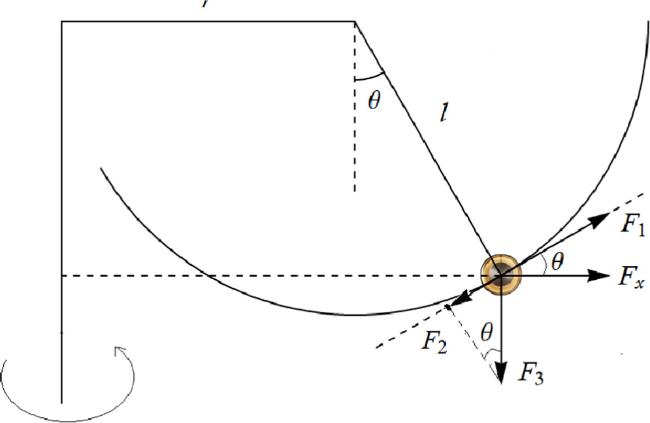
Figure 1. Rotating pendulum system with gallows. |
Some interesting limiting cases will be considered in this study
| • | For φ(t) = ϵ = φ(t) = 0: Free oscillations of the pendulum are considered and the solution of this oscillation was studied as shown in [36]. |
| • | For ω = φ(t) = 0: Normal damped simple pendulum, |
| • | For α = 0: Rotating pendulum without gallows. |
| • | For ω ≠ 0, α ≠ 0, and φ(t) ≠ 0: Forced rotating pendulum with gallows. |
2. MSM for analyzing a forced-damped rotational pendulum system
Here, we begin to analyze some cases for the stated problem, as indicated below.
2.1. First Case: Normal damped simple pendulum
For the unforced (φ(t) = 0) and un-rotational oscillator ω = 0, the original problem (1 ) reduces to the following initial value problem (i.v.p.),2 ) reduces to the following new approximation form4 ), we obtain5 ) using the MSM reads6 ) represents the first-approximation using the MSM, and for higher-order approximations, this solution can be written in the following general form
$\begin{eqnarray}\left\{\begin{array}{l}\ddot{\theta }+2\varepsilon \dot{\theta }+{\omega }_{0}^{2}\sin \theta =0,\\ \theta (0)={\theta }_{0}\,\mathrm{and}\,\dot{\theta }(0)={\dot{\theta }}_{0}.\end{array}\right.\end{eqnarray}$
Using the following approximation to $\sin \theta $, $\begin{eqnarray}\sin \theta \approx \theta -\displaystyle \frac{{\theta }^{3}}{6}+\displaystyle \frac{{\theta }^{5}}{120}.\end{eqnarray}$
then the i.v.p. ( $\begin{eqnarray}\left\{\begin{array}{l}\ddot{\theta }+2\varepsilon \dot{\theta }+{\omega }_{0}^{2}\left(\theta -\displaystyle \frac{{\theta }^{3}}{6}+\displaystyle \frac{{\theta }^{5}}{120}\right)=0,\\ \theta (0)={\theta }_{0}\,\mathrm{and}\,\dot{\theta }(0)={\dot{\theta }}_{0}.\end{array}\right.\end{eqnarray}$
Now, by considering the perturbation form to the i.v.p. ( $\begin{eqnarray}\left\{\begin{array}{l}{\mathbb{N}}\equiv \ddot{\theta }+{\omega }_{0}^{2}\theta +p\left[2\varepsilon \dot{\theta }+{\omega }_{0}^{2}\left(-\displaystyle \frac{{\theta }^{3}}{6}+\displaystyle \frac{{\theta }^{5}}{120}\right)\right]=0,\\ \theta (0)={\theta }_{0}\,\mathrm{and}\,\dot{\theta }(0)={\dot{\theta }}_{0}.\end{array}\right.\end{eqnarray}$
The first-approximation to the problem ( $\begin{eqnarray}\theta (t)={\theta }_{0}a(\tau )\cos (\varphi )+{c}_{1}a(\tau )\sin (\varphi )+{pU}(t,\tau )+O\left({p}^{2}\right),\end{eqnarray}$
where $\varphi \equiv \varphi \left(t\right)={\omega }_{0}t+\psi (\tau )$ and τ = pt. Note that solution ( $\begin{eqnarray}\begin{array}{l}\theta ={\theta }_{0}a({\tau }_{1,}{\tau }_{2,}\ldots )\cos (\varphi )\\ +{c}_{1}a({\tau }_{1,}{\tau }_{2,}\ldots )\sin (\varphi )\\ +\displaystyle \sum _{i=1}^{\infty }{p}^{i}{U}_{i}(t,{\tau }_{1,}{\tau }_{2,}\ldots ),\end{array}\end{eqnarray}$
where τi = pit and i = 1, 2, 3,….Inserting solution (6 ) into problem (5 ), implies9 ) and (10 ) into solution (6 ) for p = 1, we finally get the MSM first-approximation to the i.v.p. (2 ) as follows
$\begin{eqnarray}{\mathbb{N}}=\left({F}_{0}+{F}_{1}\sin (\varphi )+{F}_{2}\cos (\varphi )\right)p+O({p}^{2}),\ \ \ \ \ \ \end{eqnarray}$
with $\begin{eqnarray*}\begin{array}{l}{F}_{0}=\displaystyle \frac{1}{960}a{\left(\tau \right)}^{3}\left(\sin (\varphi ){c}_{1}+\cos (\varphi ){\theta }_{0}\right)+\\ +\,{\omega }_{0}^{2}U(t,\tau )+{U}^{(\mathrm{2,0})}(t,\tau )\\ +\,{\omega }_{0}^{2}\left[\begin{array}{c}a{\left(\tau \right)}^{2}\left(-2-4\cos (2\varphi )+\cos (4\varphi )\right){c}_{1}^{4}\\ +32a{\left(\tau \right)}^{2}\cos (\varphi ){\sin }^{3}(\varphi ){c}_{1}^{3}{\theta }_{0}\\ +16\sin (2\varphi ){c}_{1}{\theta }_{0}\left(-10+a{\left(\tau \right)}^{2}{\cos }^{2}(\varphi ){\theta }_{0}^{2}\right)\\ +{\theta }_{0}^{2}\left(\begin{array}{c}40-80\cos (2\varphi )\\ +a{\left(\tau \right)}^{2}\left(-2+4\cos (2\varphi )+\cos (4\varphi )\right){\theta }_{0}^{2}\end{array}\right)\\ +{c}_{1}^{2}\left(40+80\cos (2\varphi )-2a{\left(\tau \right)}^{2}(2+3\cos (4\varphi )){\theta }_{0}^{2}\right)\end{array}\right],\\ {F}_{1}=\displaystyle \frac{1}{192}{\omega }_{0}\left(\begin{array}{c}-24a{\left(\tau \right)}^{3}{c}_{1}\left({c}_{1}^{2}+{\theta }_{0}^{2}\right){\omega }_{0}+\\ a{\left(\tau \right)}^{5}{c}_{1}\left({c}_{1}^{2}+{\theta }_{0}^{2}\right){}^{2}{\omega }_{0}-384{\theta }_{0}\dot{a}(\tau )\\ -384a(\tau )\left(\varepsilon {\theta }_{0}+{c}_{1}\dot{\psi }(\tau )\right)\end{array}\right),\\ {F}_{2}=\displaystyle \frac{1}{192}{\omega }_{0}\left(\begin{array}{c}-24a{\left(\tau \right)}^{3}{\theta }_{0}\left({c}_{1}^{2}+{\theta }_{0}^{2}\right){\omega }_{0}\\ +a{\left(\tau \right)}^{5}{\theta }_{0}\left({c}_{1}^{2}+{\theta }_{0}^{2}\right){}^{2}{\omega }_{0}\\ +384{c}_{1}\dot{a}(\tau )+384a(\tau )\left(\varepsilon {c}_{1}-{\theta }_{0}\dot{\psi }(\tau )\right)\end{array}\right).\end{array}\end{eqnarray*}$
By solving the system F0 = 0 and F1 = 0 using the values a(τ) = 1 and ψ(0) = 0 and for p = 1, the values of both $\left(a,\psi \right)\equiv $ $\left(a(t),\psi (t)\right)$ are obtained as follows $\begin{eqnarray}\left\{\begin{array}{l}a={{\rm{e}}}^{-\varepsilon t},\\ \psi =\displaystyle \frac{1}{1536\varepsilon }\left[\begin{array}{l}{\omega }_{0}\left({c}_{1}^{2}+{\theta }_{0}^{2}\right){e}^{-4\varepsilon t}\left({{\rm{e}}}^{2\varepsilon t}-1\right)\\ \times \left(\left({c}_{1}^{2}+{\theta }_{0}^{2}-48\right){e}^{2\varepsilon t}+{c}_{1}^{2}+{\theta }_{0}^{2}\right)\end{array}\right].\end{array}\right.\end{eqnarray}$
Also, by solving F2 = 0 with $U(t,\tau )=U(t,t)\equiv V\left(t\right)$ using the conditions $V\left(0\right)=\dot{V}\left(0\right)=0$, we finally get the value of $V\left(t\right)$ as follows $\begin{eqnarray}V\left(t\right)=\displaystyle \frac{{{\rm{e}}}^{-5t\varepsilon }}{46080}\left(\begin{array}{l}-15\sin \left({{\rm{\Theta }}}_{-1}\right){c}_{1}^{5}+2\sin \left({{\rm{\Theta }}}_{-2}\right){c}_{1}^{5}+30\sin \left({{\rm{\Theta }}}_{+1}\right){c}_{1}^{5}\\ -3\sin \left({{\rm{\Theta }}}_{+1}\right){c}_{1}^{5}-15\sin \left({{\rm{\Theta }}}_{3}\right){c}_{1}^{5}+\sin \left(\displaystyle \frac{5{\rm{\Psi }}}{1536\varepsilon }+5{\omega }_{0}t\right){c}_{1}^{5}\\ +90\cos \left({{\rm{\Theta }}}_{+1}\right){\theta }_{0}{c}_{1}^{4}-15\cos \left({{\rm{\Theta }}}_{2}\right){\theta }_{0}{c}_{1}^{4}-45\cos \left({{\rm{\Theta }}}_{3}\right){\theta }_{0}{c}_{1}^{4}\\ +5\cos \left({{\rm{\Theta }}}_{4}\right){\theta }_{0}{c}_{1}^{4}+30\sin \left({{\rm{\Theta }}}_{-1}\right){\theta }_{0}^{2}{c}_{1}^{3}-20\sin \left({{\rm{\Theta }}}_{-2}\right){\theta }_{0}^{2}{c}_{1}^{3}\\ -60\sin \left({{\rm{\Theta }}}_{+1}\right){\theta }_{0}^{2}{c}_{1}^{3}+30\sin \left({{\rm{\Theta }}}_{2}\right){\theta }_{0}^{2}{c}_{1}^{3}+30\sin \left({{\rm{\Theta }}}_{3}\right){\theta }_{0}^{2}{c}_{1}^{3}\\ -10\sin \left({{\rm{\Theta }}}_{4}\right){\theta }_{0}^{2}{c}_{1}^{3}+240{{\rm{e}}}^{2t\varepsilon }\sin \left({{\rm{\Theta }}}_{-1}\right){c}_{1}^{3}-480{{\rm{e}}}^{2t\varepsilon }\sin \left({{\rm{\Theta }}}_{+1}\right){c}_{1}^{3}\\ +240{{\rm{e}}}^{2t\varepsilon }\sin \left({{\rm{\Theta }}}_{3}\right){c}_{1}^{3}+60\cos \left({{\rm{\Theta }}}_{+1}\right){\theta }_{0}^{3}{c}_{1}^{2}+30\cos \left({{\rm{\Theta }}}_{2}\right){\theta }_{0}^{3}{c}_{1}^{2}\\ -30\cos \left({{\rm{\Theta }}}_{3}\right){\theta }_{0}^{3}{c}_{1}^{2}-10\cos \left({{\rm{\Theta }}}_{4}\right){\theta }_{0}^{3}{c}_{1}^{2}-1440{{\rm{e}}}^{2t\varepsilon }\cos \left({{\rm{\Theta }}}_{+1}\right){\theta }_{0}{c}_{1}^{2}\\ +720{{\rm{e}}}^{2t\varepsilon }\cos \left({{\rm{\Theta }}}_{3}\right){\theta }_{0}{c}_{1}^{2}+45\sin \left({{\rm{\Theta }}}_{-1}\right){\theta }_{0}^{4}{c}_{1}+10\sin \left({{\rm{\Theta }}}_{-2}\right){\theta }_{0}^{4}{c}_{1}\\ -90\sin \left({{\rm{\Theta }}}_{+1}\right){\theta }_{0}^{4}{c}_{1}-15\sin \left({{\rm{\Theta }}}_{2}\right){\theta }_{0}^{4}{c}_{1}+45\sin \left({{\rm{\Theta }}}_{3}\right){\theta }_{0}^{4}{c}_{1}\\ +5\sin \left({{\rm{\Theta }}}_{4}\right){\theta }_{0}^{4}{c}_{1}-720{{\rm{e}}}^{2t\varepsilon }\sin \left({{\rm{\Theta }}}_{-1}\right){\theta }_{0}^{2}{c}_{1}+1440{{\rm{e}}}^{2t\varepsilon }\sin \left({{\rm{\Theta }}}_{+1}\right){\theta }_{0}^{2}{c}_{1}\\ -720{{\rm{e}}}^{2t\varepsilon }\sin \left({{\rm{\Theta }}}_{3}\right){\theta }_{0}^{2}{c}_{1}-30\cos \left({{\rm{\Theta }}}_{+1}\right){\theta }_{0}^{5}-3\cos \left({{\rm{\Theta }}}_{+1}\right){\theta }_{0}^{5}\\ +15\cos \left({{\rm{\Theta }}}_{3}\right){\theta }_{0}^{5}+\cos \left({{\rm{\Theta }}}_{4}\right){\theta }_{0}^{5}+480{{\rm{e}}}^{2t\varepsilon }\cos \left({{\rm{\Theta }}}_{+1}\right){\theta }_{0}^{3}\\ -240{{\rm{e}}}^{2t\varepsilon }\cos \left({{\rm{\Theta }}}_{3}\right){\theta }_{0}^{3}+15\cos \left({{\rm{\Theta }}}_{-1}\right){\theta }_{0}\left({\theta }_{0}^{2}-3{c}_{1}^{2}\right)\left({c}_{1}^{2}-16{{\rm{e}}}^{2t\varepsilon }+{\theta }_{0}^{2}\right)\\ +2\cos \left({{\rm{\Theta }}}_{-2}\right)\left({\theta }_{0}^{5}-10{c}_{1}^{2}{\theta }_{0}^{3}+5{c}_{1}^{4}{\theta }_{0}\right)\end{array}\right),\end{eqnarray}$
with $\begin{eqnarray*}\begin{array}{rcl}{\rm{\Psi }} & = & {\omega }_{0}{{\rm{e}}}^{-4\varepsilon t}\left({c}_{1}^{2}+{\theta }_{0}^{2}\right)\left({{\rm{e}}}^{2\varepsilon t}-1\right)\\ & & \times \left({c}_{1}^{2}\left({{\rm{e}}}^{2\varepsilon t}+1\right)+{\theta }_{0}^{2}\left({{\rm{e}}}^{2\varepsilon t}+1\right)-48{{\rm{e}}}^{2\varepsilon t}\right),\\ {{\rm{\Theta }}}_{-1} & = & \left(\displaystyle \frac{{\rm{\Psi }}}{512\varepsilon }-{\omega }_{0}t\right),{{\rm{\Theta }}}_{+1}=\left(\displaystyle \frac{{\rm{\Psi }}}{512\varepsilon }+{\omega }_{0}t\right),\\ {{\rm{\Theta }}}_{-2} & = & \left(\displaystyle \frac{5{\rm{\Psi }}}{1536\varepsilon }-{\omega }_{0}t\right),{{\rm{\Theta }}}_{2}=\left(\displaystyle \frac{5{\rm{\Psi }}}{1536\varepsilon }+{\omega }_{0}t\right),\\ {{\rm{\Theta }}}_{3} & = & \left(\displaystyle \frac{{\rm{\Psi }}}{512\varepsilon }+3{\omega }_{0}t\right),{{\rm{\Theta }}}_{4}=\left(\displaystyle \frac{5{\rm{\Psi }}}{1536\varepsilon }+5{\omega }_{0}t\right).\end{array}\end{eqnarray*}$
The value of coefficient c1 can be estimated using the following quintic equation $\begin{eqnarray}\begin{array}{l}\displaystyle \frac{1}{384}{\omega }_{0}{c}_{1}^{5}+\displaystyle \frac{1}{192}\left({\theta }_{0}^{2}-12\right){\omega }_{0}{c}_{1}^{3}\\ +\,\left(\displaystyle \frac{{\theta }_{0}^{4}{\omega }_{0}}{384}-\displaystyle \frac{{\theta }_{0}^{2}{\omega }_{0}}{16}+{\omega }_{0}\right){c}_{1}\\ -\,\varepsilon {\theta }_{0}-{\dot{\theta }}_{0}=0.\end{array}\end{eqnarray}$
Now, for ϵ = 0, we get $\begin{eqnarray}\psi =\displaystyle \frac{1}{384}{\omega }_{0}\left({c}_{1}^{2}+{\theta }_{0}^{2}-24\right)\left({c}_{1}^{2}+{\theta }_{0}^{2}\right)t.\end{eqnarray}$
By substituting the obtained values of a, ψ, and $V\left(t\right)$ given in equations ( $\begin{eqnarray}\begin{array}{l}\theta (t)={\theta }_{0}{{\rm{e}}}^{-\varepsilon t}\cos \left\{{\omega }_{0}t+\displaystyle \frac{1}{1536\varepsilon }\right.\\ \times \,\left.\left[\begin{array}{l}{\omega }_{0}\left({c}_{1}^{2}+{\theta }_{0}^{2}\right){{\rm{e}}}^{-4\varepsilon t}\left({{\rm{e}}}^{2\varepsilon t}-1\right)\\ \left(\left({c}_{1}^{2}+{\theta }_{0}^{2}-48\right){{\rm{e}}}^{2\varepsilon t}+{c}_{1}^{2}+{\theta }_{0}^{2}\right)\end{array}\right]\right\}\\ +\,{c}_{1}a(t)\sin \left\{{\omega }_{0}t+\displaystyle \frac{1}{1536\varepsilon }\right.\\ \times \,\left.\left[\begin{array}{l}{\omega }_{0}\left({c}_{1}^{2}+{\theta }_{0}^{2}\right){{\rm{e}}}^{-4\varepsilon t}\left({{\rm{e}}}^{2\varepsilon t}-1\right)\\ \left(\left({c}_{1}^{2}+{\theta }_{0}^{2}-48\right){{\rm{e}}}^{2\varepsilon t}+{c}_{1}^{2}+{\theta }_{0}^{2}\right)\end{array}\right]\right\}\end{array}\end{eqnarray}$
$\begin{eqnarray}+V\left(t\right).\end{eqnarray}$
Let us examine the subsequent numerical illustration
$\begin{eqnarray}\left\{\begin{array}{l}\ddot{\theta }(t)+0.2\dot{\theta }(t)+\sin (\theta (t))=0,\\ \theta (0)=0.3\,\mathrm{and}\,\dot{\theta }(0)=0.\end{array}\right.\end{eqnarray}$
Using solution ( $\begin{eqnarray}\begin{array}{l}\theta (t)=4.7427700280994885\times {10}^{-8}{{\rm{e}}}^{-0.5t}\\ \times \,\cos \left(-5t+{\psi }_{5}(t)\right)\\ +\,\left(7.747\,719\,281\,526\,569\times {10}^{-7}{{\rm{e}}}^{-0.5t}\right.\\ \left.-\,0.000136358{{\rm{e}}}^{-0.3t}\right)\\ \times \,\cos \left(-3t+{\psi }_{5}(t)\right)+{e}^{-0.1t}{K}_{1}\\ +\,{{\rm{e}}}^{-0.3t}{K}_{2}+{{\rm{e}}}^{-0.5t}{K}_{3}.\end{array}\end{eqnarray}$
The values of coefficients ${K}_{\mathrm{1,2,3}}$ are defined in appendix Figure 2 compares the MSM’s first-order approximation (16 ) and the numerical approximation using the RK4 method. Furthermore, the maximum error for the first-approximation (16 ) of the MSM compared to the introduced numerical approximation using the RK4 method is determined in the following manner16 ) is highly consistent with the RK4 numerical solution.
$\begin{eqnarray*}{E}_{d}=\mathop{\max }\limits_{0\lt t\lt 30}\left|{RK}4-\theta (t)\right|=0.00566076.\end{eqnarray*}$
It is clear from both figure 2 and the maximum error Ed = 0.00566076 that the MSM first-approximation (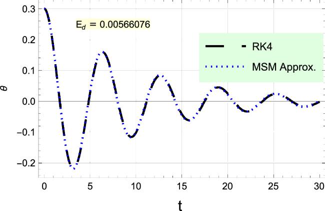
Figure 2. Comparison of the MSM first-approximation with the RK4 numerical approximation for normal damped simple pendulum, i.e., for ω = φ(t) = 0. |
2.2. Second Case: Rotational oscillator ω ≠ 0
We first solve the following unforced case17 ) is replaced with the following i.v.p.19 )20 ) into ${\mathbb{R}}$, the following i.v.p. is obtained
$\begin{eqnarray}\left\{\begin{array}{l}\ddot{\theta }+2\varepsilon \dot{\theta }+{\omega }_{0}^{2}\sin \theta -{\omega }^{2}(\alpha +\sin \theta )\cos \theta =0,\\ \theta (0)={\theta }_{0}\,\mathrm{and}\,\dot{\theta }(0)={\dot{\theta }}_{0}.\end{array}\right.\end{eqnarray}$
The following Chebyshev approximation for the terms: ${\mathbb{N}}={\omega }_{0}^{2}\sin \theta -{\omega }^{2}(\alpha +\sin \theta )\cos \theta $ for −1 ≤ θ ≤ 1, is obtained $\begin{eqnarray}{\mathbb{N}}\approx -\alpha {\omega }^{2}+q\theta +r{\theta }^{2}+s{\theta }^{3},\end{eqnarray}$
with $\begin{eqnarray*}\begin{array}{l}q=-0.0153468\alpha {\omega }^{2}-0.982489{\omega }^{2}+0.998812{\omega }_{0}^{2},\\ s=0.0153468\alpha {\omega }^{2}+0.527841{\omega }^{2}-0.157341{\omega }_{0}^{2},\\ r=0.459698\alpha {\omega }^{2}.\end{array}\end{eqnarray*}$
The i.v.p. ( $\begin{eqnarray}\left\{\begin{array}{l}{\mathbb{R}}\equiv \ddot{\theta }+2\varepsilon \dot{\theta }-\alpha {\omega }^{2}+q\theta +r{\theta }^{2}+s{\theta }^{3}=0,\\ \theta (0)={\theta }_{0}\,\mathrm{and}\,\dot{\theta }(0)={\dot{\theta }}_{0}.\end{array}\right.\end{eqnarray}$
Let the solution of problem ( $\begin{eqnarray}\theta (t)={\rm{d}}+u(t),\end{eqnarray}$
with $\begin{eqnarray*}-\alpha {\omega }^{2}+q{\rm{d}}+r{{\rm{d}}}^{2}+s{{\rm{d}}}^{3}=0.\end{eqnarray*}$
Inserting solution ( $\begin{eqnarray}\left\{\begin{array}{l}\ddot{u}+2\varepsilon \dot{u}+{P}^{2}u+{{Qu}}^{2}+{{su}}^{3}=0,\,\\ u(0)={u}_{0}:= {\theta }_{0}-{\rm{d}}\,\mathrm{and}\,\dot{u}(0)={\dot{\theta }}_{0},\end{array}\right.\end{eqnarray}$
with $\begin{eqnarray*}\left\{\begin{array}{l}{P}^{2}=3s{{\rm{d}}}^{2}+2r{\rm{d}}+q,\\ Q=(3s{\rm{d}}+r).\end{array}\right.\end{eqnarray*}$
Now, by constructing the homotopy, we get $\begin{eqnarray}{H}_{p}(t)=\ddot{u}+{P}^{2}u+p\left[2\varepsilon \dot{u}+{{Qu}}^{2}+{{su}}^{3}\right].\end{eqnarray}$
The solution is assumed in the ansatz form $\begin{eqnarray}u(t)=({\theta }_{0}-d)a(\tau )\cos (\varphi )+{c}_{1}a(\tau )\sin (\varphi )+{pU}(t,\tau ),\end{eqnarray}$
with $\begin{eqnarray*}\left\{\begin{array}{l}\varphi =({Pt}+\psi (\tau )),\\ {\theta }_{d}=({\theta }_{0}-d),\end{array}\right.\end{eqnarray*}$
where τ = pt.Inserting solution (23 ) into equation (22 ), we have21 ) is provided by27 ).
$\begin{eqnarray}{H}_{p}(t)=\left({S}_{0}+{S}_{1}\sin (\varphi )+{S}_{2}\cos (\varphi )\right)p+O({p}^{2}),\end{eqnarray}$
with $\begin{eqnarray*}\begin{array}{l}{S}_{0}=\begin{array}{c}{U}^{(\mathrm{2,0})}(t,\tau )+{P}^{2}U(t,\tau )\\ \qquad -\displaystyle \frac{1}{4}a{\left(\tau \right)}^{2}\left({c}_{1}\sin (\varphi )+{u}_{0}\cos (\varphi )\right)\\ \displaystyle \frac{1}{4}\left[\begin{array}{c}-4{c}_{1}\sin (\varphi )\left(2{{su}}_{0}a(\tau )\cos (\varphi )+Q\right)\\ +{c}_{1}^{2}{sa}(\tau )(2\cos (2\varphi )+1)\\ +{u}_{0}\left({{su}}_{0}a(\tau )(1-2\cos (2\varphi ))-4Q\cos (\varphi )\right)\end{array}\right]\end{array},\\ {S}_{1}=\displaystyle \frac{1}{4}\left[\begin{array}{l}-8{u}_{0}P\dot{a}(\tau )+3{c}_{1}{sa}{\left(\tau \right)}^{3}\left({c}_{1}^{2}+{u}_{0}^{2}\right)\\ -8{Pa}(\tau )\left({c}_{1}\dot{\psi }(\tau )+\varepsilon {u}_{0}\right)\end{array}\right]\sin (\varphi ),\\ {S}_{2}=\displaystyle \frac{1}{4}\left[\begin{array}{l}8{c}_{1}P\dot{a}(\tau )+3{{su}}_{0}a{\left(\tau \right)}^{3}\left({c}_{1}^{2}+{u}_{0}^{2}\right)\\ +8{Pa}(\tau )\left({c}_{1}\varepsilon -{u}_{0}\dot{\psi }(\tau )\right)\end{array}\right]\cos (\varphi ).\end{array}\end{eqnarray*}$
By solving the system S1 = 0 and S2 = 0, the values of $\left(a,\psi \right)$ are obtained as follow $\begin{eqnarray}\left\{\begin{array}{c}a={{\rm{e}}}^{-\varepsilon \tau },\\ \psi =\displaystyle \frac{3s\left({c}_{1}^{2}+{u}_{0}^{2}\right)}{8\varepsilon P}{{\rm{e}}}^{-\varepsilon \tau }\sinh (\varepsilon \tau ).\end{array}\right.\end{eqnarray}$
Also, by solving S0 = 0, $\begin{eqnarray}\begin{array}{l}{U}^{(\mathrm{2,0})}(t,\tau )+{P}^{2}U(t,\tau )=\displaystyle \frac{1}{4}a{\left(\tau \right)}^{2}\left({c}_{1}\sin \left(\varphi \right)+{u}_{0}\cos \left(\varphi \right)\right)\\ \times \left\{\begin{array}{c}-4{c}_{1}\sin (\varphi )\left(2{{su}}_{0}a(\tau )\cos (\varphi )+Q\right)\\ +{c}_{1}^{2}{sa}(\tau )(2\cos (2\varphi )+1)\\ +{u}_{0}\left[{{su}}_{0}a(\tau )\left(1-2\cos (2\varphi )\right)-4Q\cos (\varphi )\right]\end{array}\right\},\end{array}\end{eqnarray}$
the value of U(t, τ) is obtained as $\begin{eqnarray}U(t,\tau )={W}_{1}{a}^{2}+{W}_{2}{a}^{3}s,\end{eqnarray}$
with $\begin{eqnarray*}\begin{array}{rcl}{W}_{1} & = & \displaystyle \frac{Q}{3{P}^{2}}\left\{\begin{array}{c}\left[\begin{array}{c}{c}_{1}{\theta }_{d}\left(\sin \left(2\varphi \right)-\cos \left({Pt}\right)\sin (2\psi (t))\right)\\ +{c}_{1}^{2}\left({\sin }^{2}\left(\varphi \right)-\cos \left({Pt}\right){\sin }^{2}(\psi (t))\right)+\\ +{\theta }_{d}{}^{2}\left({\cos }^{2}\left(\varphi \right)-\cos \left({Pt}\right){\cos }^{2}(\psi (t))\right)\end{array}\right]\\ +\sin \left({Pt}\right)\left[\begin{array}{c}\left({\theta }_{d}{}^{2}-{c}_{1}^{2}\right)\sin (2\psi (t))\\ -2{c}_{1}{\theta }_{d}\cos (2\psi (t))\end{array}\right]\\ +2\left({c}_{1}^{2}+{\theta }_{d}{}^{2}\right)\left(\cos \left({Pt}\right)-1\right)\end{array}\right\},\\ {W}_{2} & = & \displaystyle \frac{1}{32{P}^{2}}\left\{\begin{array}{c}\left[\begin{array}{c}3{c}_{1}{\theta }_{d}{}^{2}\sin \left(3\left(\varphi \right)\right)-3{c}_{1}^{2}{\theta }_{d}\cos \left(3\left(\varphi \right)\right)\\ +{c}_{1}^{3}\left(-\sin \left(3\left(\varphi \right)\right)\right)+{\theta }_{d}{}^{3}\cos \left(3\left(\varphi \right)\right)\end{array}\right]\\ +\cos \left({Pt}\right)\left[\begin{array}{c}{c}_{1}\left({c}_{1}^{2}-3{\theta }_{d}{}^{2}\right)\sin (3\psi (t))\\ -{\theta }_{d}\left({\theta }_{d}{}^{2}-3{c}_{1}^{2}\right)\cos (3\psi (t))\end{array}\right]\\ +3\sin \left({Pt}\right)\left[\begin{array}{c}{\theta }_{d}\left({\theta }_{d}{}^{2}-3{c}_{1}^{2}\right)\sin (3\psi (t))\\ +{c}_{1}\left({c}_{1}^{2}-3{\theta }_{d}{}^{2}\right)\cos (3\psi (t))\end{array}\right]\end{array}\right\}.\end{array}\end{eqnarray*}$
The value of c1 is determined through the solution of the given cubic equation $\begin{eqnarray}3{{sc}}_{1}^{3}+\left(8{P}^{2}+3s{\theta }_{d}{}^{2}\right){c}_{1}+8P\left(d\varepsilon -\varepsilon {\theta }_{0}-{\dot{\theta }}_{0}\right)=0.\end{eqnarray}$
Hence, the final solution to the i.v.p. ( $\begin{eqnarray}\begin{array}{l}\theta (t)={\rm{d}}+{\theta }_{d}{{\rm{e}}}^{-\varepsilon t}\cos \left[{Pt}+\displaystyle \frac{3s\left({c}_{1}^{2}+{u}_{0}^{2}\right)}{8\varepsilon P}{{\rm{e}}}^{-\varepsilon t}\sinh (\varepsilon t)\right]\\ +{c}_{1}{{\rm{e}}}^{-\varepsilon t}\sin \left[{Pt}+\displaystyle \frac{3s\left({c}_{1}^{2}+{u}_{0}^{2}\right)}{8\varepsilon P}{{\rm{e}}}^{-\varepsilon t}\sinh (\varepsilon t)\right]+U(t),\end{array}\end{eqnarray}$
where the value of U(t) is given in equation (Considering the following numerical example
$\begin{eqnarray}\left\{\begin{array}{c}\ddot{\theta }+0.2\dot{\theta }+\sin (\theta )-{0.2}^{2}(2+\sin (\theta ))\cos (\theta )=0,\\ \theta (0)=0.3\ \mathrm{and}\,\dot{\theta }(0)=0,\end{array}\right.\end{eqnarray}$
and by applying solution ( $\begin{eqnarray}\theta ={{\rm{e}}}^{-0.1t}{G}_{1}+{{\rm{e}}}^{-0.2t}{G}_{2}+{{\rm{e}}}^{-0.3t}{G}_{3}.\end{eqnarray}$
The values of coefficients ${G}_{\mathrm{1,2,3}}$ are defined in appendix In figure 3, we examine the contrast between the first-order approximation (31 ) using the MSM and the numerical approximation using the RK4 method for the i.v.p. (30 ). The two solutions exhibit perfect similarity. Moreover, the maximum error for the first-order approximation (31 ) of the MSM compared to the introduced numerical approximation using the RK4 method is determined in the following manner
$\begin{eqnarray*}{E}_{d}=\mathop{\max }\limits_{0\lt t\lt 30}\left|{RK}4-\theta (t)\right|=0.0034489.\end{eqnarray*}$
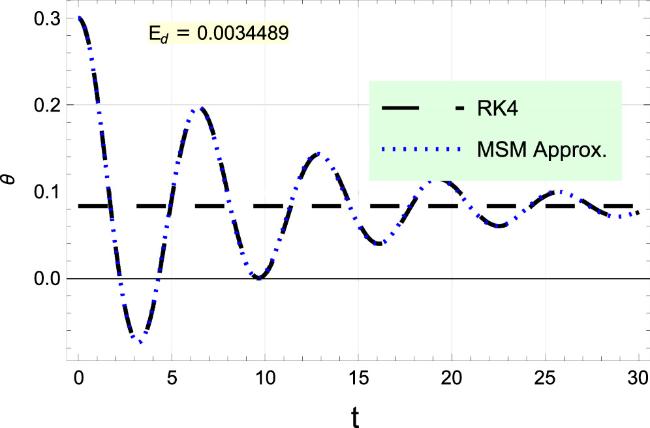
Figure 3. This figure presents a comparative analysis between the first-order approximation using the MSM and the RK4 numerical approximation technique for solving the damped rotating oscillator equation with gallows ω ≠ 0 and α ≠ 0. |
Let’s compare the used method (MSM) with recently published methods to assess its correctness. For instance, we can contrast our present approach (MSM) with the He-MSM [37] across various angular velocity ‘ω’ and the parameter responsible for gallows ‘α’, encompassing low and high values. Typically, both procedures yield comparable outcomes for small values of $\left(\alpha ,\omega \right)$. However, upon closer examination, it becomes apparent that the He-MSM differs from the currently used method (MSM) primarily at small values to $\left(\alpha ,\omega \right)$ as shown in figure 4. Conversely, the presently used method (MSM) exhibits greater accuracy than He-MSM at large values of $\left(\alpha ,\omega \right)$, displaying a significant disparity from the He-MSM, which is evident in figure 5. Additionally, the maximum errors for the second-order approximations using both MSM and He-MSM are estimated and compared to the RK4 numerical approximation:
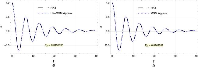
Figure 4. This figure presents a comparative analysis between the second-order approximations using both MSM and He-MSM for solving the damped rotating oscillator equation with gallows. Here, $\left(\alpha ,\omega \right)=\left(1,0.1\right).$ |
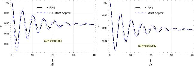
Figure 5. This figure presents a comparative analysis between the second-order approximations using both MSM and He-MSM for solving the damped rotating oscillator equation with gallows. Here, $\left(\alpha ,\omega \right)=\left(2,0.67\right).$ |
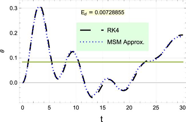
Figure 6. This figure presents a comparative analysis between the first-approximation using the MSM and the RK4 numerical approximation technique for solving the forced-damped rotating oscillator, i.e., for ω ≠ 0, α ≠ 0, and φ(t) ≠ 0. |
for $\left(\alpha ,\omega \right)=\left(1,0.2\right)$
$\begin{eqnarray*}\begin{array}{rcl}{\left.{E}_{d}\right|}_{\mathrm{He}-\mathrm{MsM}} & = & \mathop{\max }\limits_{0\lt t\lt 30}\left|{RK}4-\theta (t)\right|\,=\,0.0155835,\\ {\left.{E}_{d}\right|}_{\mathrm{MsM}} & = & \mathop{\max }\limits_{0\lt t\lt 30}\left|{RK}4-\theta (t)\right|=0.0255316,\end{array}\end{eqnarray*}$
and for $\left(\alpha ,\omega \right)=\left(2,0.67\right)$ $\begin{eqnarray*}\begin{array}{rcl}{\left.{E}_{d}\right|}_{\mathrm{He}-\mathrm{MsM}} & = & \mathop{\max }\limits_{0\lt t\lt 30}\left|{RK}4-\theta (t)\right|\,=\,0.0481151,\\ {\left.{E}_{d}\right|}_{\mathrm{MsM}} & = & \mathop{\max }\limits_{0\lt t\lt 30}\left|{RK}4-\theta (t)\right|=0.0322512.\end{array}\end{eqnarray*}$
2.3. Third case: Forced rotational pendulum: φ(t) ≠ 0
In this case, all effects are considered in addition to taking the external excited force into consideration32 ) can be assumed to have the following form32 ) for φ(t) = 0, i.e.,34 ) is obtained above using MSM, while the approximate solution to the i.v.p. (35 ) can be determined easily using MATHEMATICA command ‘DSolve’ as follows
$\begin{eqnarray}\left\{\begin{array}{c}\ddot{\theta }+2\varepsilon \dot{\theta }+{\omega }_{0}^{2}\sin \left(\theta \right)-{\omega }^{2}(\alpha +\sin \left(\theta \right))\cos \left(\theta \right)={\phi }(t),\\ \theta (0)={\theta }_{0}\,\mathrm{and}\,\dot{\theta }(0)={\dot{\theta }}_{0}.\end{array}\right.\end{eqnarray}$
The approximation to problem ( $\begin{eqnarray}\theta ={\rm{\Phi }}\left(t\right)+y\left(t\right),\end{eqnarray}$
where ${\rm{\Phi }}\equiv {\rm{\Phi }}\left(t\right)$ represents the solution of problem ( $\begin{eqnarray}\left\{\begin{array}{c}\ddot{{\rm{\Phi }}}+2\varepsilon \dot{{\rm{\Phi }}}+{\omega }_{0}^{2}\sin \left({\rm{\Phi }}\right)-{\omega }^{2}(\alpha +\sin \left({\rm{\Phi }}\right))\cos \left({\rm{\Phi }}\right)=0,\\ {\rm{\Phi }}(0)={\theta }_{0}\,\mathrm{and}\,\dot{{\rm{\Phi }}}(0)={\dot{\theta }}_{0},\end{array}\right.\end{eqnarray}$
whereas $y\equiv y\left(t\right)$ indicates the solution to the following i.v.p. $\begin{eqnarray}\left\{\begin{array}{c}\ddot{y}+2\varepsilon \dot{y}+{\omega }_{0}^{2}y={\phi }(t),\\ y(0)={\theta }_{0}\,\mathrm{and}\,\dot{y}(0)={\dot{\theta }}_{0}.\end{array}\right.\end{eqnarray}$
The solution of the i.v.p. ( $\begin{eqnarray*}\begin{array}{l}\quad Y\left[t\_\right]:= {y}^{{\prime\prime} }\left[t\right]+2\,\mathrm{EulerGamma}{y}^{{\prime} }\left[t\right]\\ \quad +{\mathrm{Catalan}}^{2}y\left[t\right]=={\phi }\left[t\right]\\ \mathrm{Simplify}[\mathrm{Solve}[Y\left[t\right]\&\&y\left[0\right]=={y}^{{\prime} }\left[0\right]==0,y\left[t\right],t]]//.\\ \left\{\mathrm{EulerGamma}\to \varepsilon ,\mathrm{Catalan}\to {\omega }_{0},K[j\_]:\to \,\tau \right\}\end{array}\end{eqnarray*}$
which leads to $\begin{eqnarray}y={{\rm{e}}}^{-\varepsilon t}\left[\begin{array}{c}\sin \left(t{\omega }_{\varepsilon }\right)\left({\displaystyle \int }_{1}^{t}{{\rm{\Gamma }}}_{1}\left(\tau \right)d\tau -{\displaystyle \int }_{1}^{0}{{\rm{\Gamma }}}_{1}\left(\tau \right)d\tau \right)\\ +\cos \left(t{\omega }_{\varepsilon }\right)\left({\displaystyle \int }_{1}^{t}{{\rm{\Gamma }}}_{2}\left(\tau \right)d\tau -{\displaystyle \int }_{1}^{0}{{\rm{\Gamma }}}_{2}\left(\tau \right)d\tau \right)\end{array}\right],\end{eqnarray}$
with $\begin{eqnarray*}\begin{array}{rcl}{{\rm{\Gamma }}}_{1}\left(\tau \right) & = & \displaystyle \frac{{{\rm{e}}}^{\varepsilon \tau }{\phi }(\tau )}{{\omega }_{\varepsilon }}\cos \left(\tau {\omega }_{\varepsilon }\right),\\ {{\rm{\Gamma }}}_{2}\left(\tau \right) & = & -\displaystyle \frac{{{\rm{e}}}^{\varepsilon \tau }{\phi }(\tau )}{{\omega }_{\varepsilon }}\sin \left(\tau {\omega }_{\varepsilon }\right),\end{array}\end{eqnarray*}$
where ${\omega }_{\varepsilon }=\sqrt{{\omega }_{0}^{2}-{\varepsilon }^{2}}$.For the first simplification to the solution (36 ), we get37 ) into the solution (33 ), we finally get an approximation to the i.v.p. (32 ) as follows39 ) and the RK4 numerical approximation for $\left(\varepsilon ,\alpha ,{\omega }_{0},\omega ,{\theta }_{0},{\dot{\theta }}_{0}\right)=\left(0.1,2,1,0.2,0,0\right)$ and ${\phi }(\tau )={\rm{\Gamma }}\cos \left({\rm{\Omega }}t\right)=0.1\cos \left(0.2t\right)$ are presented in figure 6. Also, the maximum error Ed to the approximation (39 ) as compared to the RK4 numerical approximation is estimated: Ed = 0.00728855. It is clear from both the calculated error Ed, in addition to the comparison results as shown in figure 6, that the two approximations are compatible for a long time. The numerical value of solution (39 ) according to the mentioned data given byC .
$\begin{eqnarray}y={{\rm{e}}}^{-\varepsilon t}\left\{{\int }_{0}^{t}\left(\sin \left(t{\omega }_{\varepsilon }\right){{\rm{\Gamma }}}_{1}\left(\tau \right)+\cos \left(t{\omega }_{\varepsilon }\right){{\rm{\Gamma }}}_{2}\left(\tau \right)\right)d\tau \right\}.\end{eqnarray}$
For more simplification, we have $\begin{eqnarray}y=\displaystyle \frac{1}{{\omega }_{\varepsilon }}{\int }_{0}^{t}{{\rm{e}}}^{\varepsilon \left(\tau -t\right)}{\phi }(\tau )\sin \left[\left(t-\tau \right){\omega }_{\varepsilon }\right]d\tau .\end{eqnarray}$
Now, by inserting the value of y given in equation ( $\begin{eqnarray}\theta (t)={\rm{\Phi }}\left(t\right)+\displaystyle \frac{1}{{\omega }_{\varepsilon }}{\int }_{0}^{t}{{\rm{e}}}^{\varepsilon \left(\tau -t\right)}{\phi }(\tau )\sin \left[\left(t-\tau \right){\omega }_{\varepsilon }\right]d\tau .\end{eqnarray}$
The approximation ( $\begin{eqnarray}\begin{array}{l}\theta (t)=0.0832976+0.00433276\sin (0.2t)\\ \quad +0.103986\cos (0.2t)+{{\mathbb{Z}}}_{1}{{\rm{e}}}^{-0.1t}+{{\mathbb{Z}}}_{2}{{\rm{e}}}^{-0.2t}+{{\mathbb{Z}}}_{3}{{\rm{e}}}^{-0.3t}\end{array}\end{eqnarray}$
The values of coefficients ${{\mathbb{Z}}}_{\mathrm{1,2,3}}$ are defined in appendix 3. Conclusions
A generalized forced-damped rotational pendulum system [35] has been investigated analytically via the multiple scales method (MSM). The proposed problem has been divided into three cases/oscillators to analyze each case separately. In this first case, the MSM has been applied directly to find an approximation to the standard simple pendulum with damping term/friction force ϵ ≠ 0, i.e., for ω = φ(t) = 0. The first-order approximations were derived and analyzed using some concrete numerical examples. In the second case/oscillator, the effects of both rotational and gallows are considered, and the MSM first-order approximation for this oscillator was derived and discussed based on some numerical examples. In the third case/oscillator, the MSM first-order approximation was derived for the generalized forced-damped rotational pendulum oscillator. Furthermore, a comparison has been made between the numerical approximations obtained by the fourth-order Runge–Kutta (RK4) method and the first-order approximations derived from the MSM for three cases of the problem under consideration. Moreover, the comparison findings between the conventional MSM and the He-MSM have demonstrated that both approaches exhibit a satisfactory correlation at small values of $\left(\alpha ,\omega \right)$. Nevertheless, He-MSM shows a tiny advantage over standard MSM when dealing with small values of $\left(\alpha ,\omega \right)$. Conversely, at large values of $\left(\alpha ,\omega \right)$, the regular MSM significantly outperforms the He-MSM.
The results indicate that the analytical and numerical approximations are in complete agreement. Moreover, the maximum distance error has been estimated. It has been observed that analytical approximations exhibit a high level of accuracy and just slight errors, thus demonstrating the efficacy of the MSM in evaluating various highly nonlinear oscillators. In that sense, this methodology allows us to determine the behavior of long-term solutions. It opens ways to assess the stability solutions and perform a qualitative analysis of said system.
Author declarations
Data availability
All data generated or analyzed during this study are included in this published article (More details or codes can be requested from El-Tantawy).
Author contributions statement
Conceptualization, H A Alyousef and A H Salas; Methodology, A H Salas and S A El-Tantawy; Software, H A Alyousef and B M Alotaibi; Validation, A H Salas and S A El-Tantawy; Formal analysis, H A Alyousef and B M Alotaibi; Investigation, A H Salas and S A El-Tantawy; Resources, H A Alyousef and B M Alotaibi; Writing—original draft, H A Alyousef and B M Alotaibi; Writing—review & editing, A H Salas and S A El-Tantawy.
Conflicts of interest
The authors declare that they have no conflicts of interest.
Appendix A. The coefficients K1,2,3 of solution (16 )
$\begin{eqnarray*}\begin{array}{l}{K}_{1}=\left(0.3\cos \left(-t+{\psi }_{4}(t)\right)-0.0301708\sin \left(-t+{\psi }_{4}(t)\right)\right),\\ {K}_{2}=\left(\begin{array}{c}0.0000422846\sin \left(-3t+{\psi }_{3}(t)\right)-0.0000845692\sin \left(-t+{\psi }_{3}(t)\right)\\ +0.0000422846\sin \left(t+{\psi }_{3}(t)\right)+0.000272716\cos \left(-t+{\psi }_{3}(t)\right)\\ -0.000136358\cos \left(t+{\psi }_{3}(t)\right)\end{array}\right),\end{array}\end{eqnarray*}$
and $\begin{eqnarray*}{K}_{3}=\left(\begin{array}{c}-2.598142668899252\times {10}^{-8}\sin \left(-5t+{\psi }_{5}(t)\right)\\ -2.402566312570247\times {10}^{-7}\sin \left(-3t+{\psi }_{3}(t)\right)\\ +7.794428006697758\times {10}^{-8}\sin \left(-t+{\psi }_{5}(t)\right)\\ +4.805132625140494\times {10}^{-7}\sin \left(-t+{\psi }_{3}(t)\right)\\ -5.196285337798504\times {10}^{-8}\sin \left(t+{\psi }_{5}(t)\right)\\ -2.402566312570247\times {10}^{-7}\sin \left(t+{\psi }_{3}(t)\right)\\ -1.4228310084298466\times {10}^{-7}\cos \left(-t+{\psi }_{5}(t)\right)\\ -1.5495438563053139\times {10}^{-6}\cos \left(-t+{\psi }_{3}(t)\right)\\ +9.48554005619898\times {10}^{-8}\cos \left(t+{\psi }_{5}(t)\right)\\ +7.747719281526569\times {10}^{-7}\cos \left(t+{\psi }_{3}(t)\right)\end{array}\right),\end{eqnarray*}$
with $\begin{eqnarray*}\begin{array}{l}{\psi }_{3}(t)=0.000161419{e}^{-0.4t}\\ -0.0852284{e}^{-0.2t}+0.085067,\\ {\psi }_{4}(t)=0.0000538065{e}^{-0.4t}\\ -0.0284095{e}^{-0.2t}+0.0283557,\\ {\psi }_{5}(t)=0.000269032{e}^{-0.4t}\\ -0.142047{e}^{-0.2t}+0.141778.\end{array}\end{eqnarray*}$
Appendix B. The coefficients G1,2,3 of solution (31 )
$\begin{eqnarray*}\begin{array}{l}{G}_{1}=\left(\begin{array}{c}0.216702\cos \left(-0.980613t+{{\rm{\Pi }}}_{2}\right)\\ -0.022154\sin \left(-0.980613t+{{\rm{\Pi }}}_{2}\right)\end{array}\right),\\ {G}_{2}=\left(\begin{array}{c}-5.059\times {10}^{-6}\sin \left(-1.96123t+{{\rm{\Pi }}}_{3}\right)\\ +7.589\times {10}^{-6}\sin \left(-0.980613t+{{\rm{\Pi }}}_{3}\right)\\ -2.529\times {10}^{-6}\sin \left(0.980\,613t+{{\rm{\Pi }}}_{3}\right)\\ +0.0000244866\cos \left(-1.96123t+{{\rm{\Pi }}}_{3}\right)\\ -0.0000367299\cos \left(-0.980613t+{{\rm{\Pi }}}_{3}\right)\\ +0.0000122433\cos \left(0.980\,613t+{{\rm{\Pi }}}_{3}\right)\\ +0.0000750116\cos (0.980613t)\end{array}\right),\end{array}\end{eqnarray*}$
and $\begin{eqnarray*}{G}_{3}=\left(\begin{array}{c}-0.0000750116{e}^{0.1t}+0.0832976{e}^{0.3t}\\ +0.000013645\sin \left(-2.94184t+{{\rm{\Pi }}}_{1}\right)\\ -0.00002729\sin \left(-0.980613t+{{\rm{\Pi }}}_{1}\right)\\ +0.000013645\sin \left(0.980\,613t+{{\rm{\Pi }}}_{1}\right)\\ -0.0000432459\cos \left(-2.94184t+{{\rm{\Pi }}}_{1}\right)\\ +0.0000864918\cos \left(-0.980613t+{{\rm{\Pi }}}_{1}\right)\\ -0.0000432459\cos \left(0.980\,613t+{{\rm{\Pi }}}_{1}\right)\end{array}\right),\end{eqnarray*}$
with $\begin{eqnarray*}\begin{array}{l}{{\rm{\Pi }}}_{1}=-0.0367453{e}^{-0.2t}+0.0367453,\\ {{\rm{\Pi }}}_{2}=-0.0122484{e}^{-0.2t}+0.0122484,\\ {{\rm{\Pi }}}_{3}=0.0244969{e}^{-0.2t}+0.0244969.\end{array}\end{eqnarray*}$
Appendix C. The coefficients ${{\mathbb{Z}}}_{\mathrm{1,2,3}}$ of solution (40 )
$\begin{eqnarray*}\begin{array}{c}{{\mathbb{Z}}}_{1}=\left(\begin{array}{c}0.00849758\sin \left(-0.980613t+{{\rm{\Delta }}}_{3}\right)\\ -0.0832976\cos \left(-0.980613t{{\rm{\Delta }}}_{3}\right)\\ -0.103986\cos (0.994987t)-0.0113219\sin (0.994987t)\end{array}\right),\\ {{\mathbb{Z}}}_{2}=\left(\begin{array}{c}-7.4\times {10}^{-7}\sin \left(-1.96123t+{{\rm{\Delta }}}_{2}\right)\\ +1.119\times {10}^{-6}\sin \left(-0.980613t+{{\rm{\Delta }}}_{2}\right)\\ -3.73\times {10}^{-7}\sin \left(0.980\,613t+{{\rm{\Delta }}}_{2}\right)\\ +3.618\times {10}^{-6}\cos \left(-1.96123t+{{\rm{\Delta }}}_{2}\right)\\ -5.427\times {10}^{-6}\cos \left(-0.980613t+{{\rm{\Delta }}}_{2}\right)\\ +1.809\times {10}^{-6}\cos \left(0.980\,613t+{{\rm{\Delta }}}_{2}\right)\\ +0.0000110827\cos (0.980613t)-0.0000110827\end{array}\right),\end{array}\end{eqnarray*}$
and $\begin{eqnarray*}{{\mathbb{Z}}}_{3}=\left(\begin{array}{c}-7.733\times {10}^{-7}\sin \left(-2.94184t+{{\rm{\Delta }}}_{1}\right)\\ +1.5466\times {10}^{-6}\sin \left(-0.980613t+{{\rm{\Delta }}}_{1}\right)\\ -7.733\times {10}^{-7}\sin \left(0.980\,613t+{{\rm{\Delta }}}_{1}\right)\\ +2.456\times {10}^{-6}\cos \left(-2.94184t+{{\rm{\Delta }}}_{1}\right)\\ -4.913\times {10}^{-6}\cos \left(-0.980613t+{{\rm{\Delta }}}_{1}\right)\\ +2.456\times {10}^{-6}\cos \left(0.980\,613t+{{\rm{\Delta }}}_{1}\right)\end{array}\right),\end{eqnarray*}$
with $\begin{eqnarray*}\begin{array}{l}{{\rm{\Delta }}}_{1}=-0.00542901{e}^{-0.2t}+0.00542901,\\ {{\rm{\Delta }}}_{2}=-0.00361934{e}^{-0.2t}+0.00361934,\\ {{\rm{\Delta }}}_{3}=-0.00180967{e}^{-0.2t}+0.00180967.\end{array}\end{eqnarray*}$