Welcome to visit Communications in Theoretical Physics,
Gravitation Theory, Astrophysics and Cosmology

On the existence and stability of traversable wormhole solutions with novel shapefunctions in the framework of ${ \mathcal F }({ \mathcal R },{{\mathscr{L}}}_{m})$ gravity

  • Sourav Chaudhary , 1 ,
  • Jitendra Kumar , 1, ,
  • S K Maurya , 2, ,
  • Sweeti Kiroriwal , 1 ,
  • Abdul Aziz , 2
Expand
  • 1Department of Mathematics, Central University of Haryana, Jant-Pali, Mahendergarh, India
  • 2Department of Mathematical and Physical Sciences, College of Arts and Science, University of Nizwa, P.O. Box 33, Nizwa 616, Oman

Authors to whom any correspondence should be addressed.

Received date: 2023-10-30

  Revised date: 2024-03-15

  Accepted date: 2024-03-19

  Online published: 2024-05-02

Copyright

© 2024 Institute of Theoretical Physics CAS, Chinese Physical Society and IOP Publishing

Abstract

In this work, we have explored wormhole (WH) solutions in ${ \mathcal F }({ \mathcal R },{{\mathscr{L}}}_{m})$ gravity by assuming the Morris–Thorne WH metric and ${ \mathcal F }({ \mathcal R },{{\mathscr{L}}}_{m})=\tfrac{{ \mathcal R }}{2}+(1+\gamma { \mathcal R }){{\mathscr{L}}}_{m}$, where γ is the free model parameter. We determined the WH solutions by utilizing two newly developed shape functions (SF) that satisfy all basic conditions for a WH’s physical validity. We also observe that the null energy condition (NEC) behaves negatively. Finally, for both models, we use the volume integral quantifier (${ \mathcal V }{ \mathcal I }{ \mathcal Q }$) and Tolman–Oppenheimer–Volkoff (TOV) equation to determine how much exotic matter is needed near the WH throat and the stability of the WH. The extensive detailed discussions of the matter components have been done via graphical analysis. The obtained WH geometries meet the physically acceptable conditions for a stable wormhole.

Cite this article

Sourav Chaudhary , Jitendra Kumar , S K Maurya , Sweeti Kiroriwal , Abdul Aziz . On the existence and stability of traversable wormhole solutions with novel shapefunctions in the framework of ${ \mathcal F }({ \mathcal R },{{\mathscr{L}}}_{m})$ gravity[J]. Communications in Theoretical Physics, 2024 , 76(5) : 055403 . DOI: 10.1088/1572-9494/ad3544

1. Introduction

In 1916, Karl Schwarzschild had produced two distinguished papers [1, 2] cultivating Einstein’s most fertile paper [3] and exploring the exterior vacuum solution and interior solution for the static spherically symmetric metric. In the same year, a more transparent and geometric depiction of the outcomes of the papers of Einstein and Schwarzschild was presented by L. Flamm [4]. In particular, he portrayed a parabola of revolution with two asymptotically flat ends, which actually provides a glimpse of the Einstein–Rosen bridge [5], a gateway to another region of spacetime. This marked the commencement of the study of the wormhole (WH), a theoretical tube-shaped structure with asymptotically flat ends and a throat connecting them. In the last two decades, the study of exploring WH solutions has attracted a lot of attention within modern astronomy. With mathematical intuition, Morris and Thorne [6] had shown the existence of human-traversable WHs. They presented the exact solutions of general relativity (GR) and its static, traversable WHs that characterize interstellar travel corresponding structure ruled out the requirement of an event horizon. The study shows the null energy condition (NEC) violation, invalidating the physical laws for the material involved. So, in order to attain traversability, this led to the consideration of the existence of such a type of matter known as ‘exotic matter’. This raises unsolved questions regarding the actual existence of these WHs. Subsequently, numerous initiatives were launched to address this problem [711]. WHs are hypothetical topologically framed constructions that serve as a spacetime tube. Static and non-static WHs are two types of WHs that are categorized according to the throat type. In contrast to a non-static WH, which has a variable radius, a static WH has a constant throat radius. Even a photon could not cross the Einstein–Rosen bridge, according to Fuller and Wheeler [12], because it would immediately disintegrate after production. Morris et al [13] further suggested that unusual types of substance strung through a WH might keep it open, although it is unknown if such conditions are physically possible. WHs can be categorized into three subspecies, to put it simply. First of all, the common WH that violates the NEC is non-asymptotically flat, includes a singularity, and is hence impassable. The second class, which may be achieved by selecting the shape function (SF) or redshift function in the right way, is the traversable WH. The thin shell WH, which is fully traversable and geodesically complete, is the third. It is feasible to insert a shell onto the junction surface here utilizing the so-called cut-and-paste technique [14]. Due to the fact that it simply requires exotic matter for the shell and ignores the existence of any horizon, this particular class has drawn a lot of interest. To permit avoiding unusual matter, some works [1519] adopted the thin shell formalism. Along with GR, a number of WH solutions have been studied in modified gravity because of their significant advantage for which the geometrical sector of the field equations can be extended to totally eliminate the possibility of exotic matter. The following works [2029] contain several WH solutions in various adjusted gravities.
Morris and Thorne [13] demonstrated that WHs with exotic materials and a small surface area that satisfy the flare-out requirement might be traversable. However, the material content required for the WH is an exotic matter which is in violation of the null energy conditions (NEC). Actually, WH solutions violate all energy conditions in the framework of GR. From the standpoint of quantum gravity, this sort of hypothetical matter can be found as a normal consequence due to changes in the spacetime topology [30]. So, if one wants to prevent energy conditions from being violated, it is crucial to reduce the amount of exotic materials at the throat. Therefore, WHs are tested for many gravity theories like extended theories of gravity [31, 32]. Studies in scalar-tensor theories produced WH solutions [3335], in which the scalar fields play the role of a phantom fluid. In one such important work [36], observational data has been employed within the framework of matter-coupling gravity formalism to explore the potential existence of a WH solution in the galactic halo attributed to dark matter. Recently, Mustafa et al [37] investigated WH geometry in the dark matter halo region under symmetric teleparallel gravity.
Now, we intend to study WH solutions with the motivation of finding the minimal presence of exotic matter at the throat in the framework of ${ \mathcal F }({ \mathcal R },{{\mathscr{L}}}_{m})$ gravity. At first, it is proposed that a modification can be added to the ${ \mathcal F }({ \mathcal R })$ modified gravity that explicitly couples the matter Lagrangian term ${{\mathscr{L}}}_{m}$ [38] and the arbitrary function of the Ricci curvature ${ \mathcal R }$. In this regard, important applications in astronomy and cosmology for cosmological models [3942] with non-minimal curvature-matter couplings are noteworthy. Later, Harko and Lobo [43] presented a modified gravity (MoG) referred to as ${ \mathcal F }({ \mathcal R },{{\mathscr{L}}}_{m})$, which follows inevitable consequences such as the covariant divergence of energy-momentum tensor does not disappear, the motion of the test particle is non-geodesic, and an extra force orthogonal to four velocities develops.
The work is presented as follows: section 2 provides a formulation of field equations in ${ \mathcal F }({ \mathcal R },{{\mathscr{L}}}_{m})$ gravity, and section 3 describes the geometry of a WH. In sections 4, 5 and 6, energy conditions and WH models based on two shape functions are presented respectively. Furthermore, in sections 7 and 8, equilibrium conditions and volume integral quantifier (${ \mathcal V }{ \mathcal I }{ \mathcal Q }$) are determined to examine the stability and presence of exotic matter. Finally, in section 9, we sum up our findings.

2. ${ \mathcal F }({ \mathcal R },{{\mathscr{L}}}_{m})$-Gravity and field equations

The equation that governs ${ \mathcal F }({ \mathcal R },{{\mathscr{L}}}_{m})$ gravity theory can be described by action [43], having the following form,
$\begin{eqnarray}{{\mathscr{H}}}_{g}=\int { \mathcal F }({ \mathcal R },{{\mathscr{L}}}_{m})\sqrt{-{\mathfrak{g}}}\,{{\rm{d}}}^{4}x,\end{eqnarray}$
where ${ \mathcal R }$ represents the Ricci scalar complementary to the ${{\mathfrak{g}}}_{\xi \eta }$ and ${{\mathscr{L}}}_{m}$ shows the matter Lagrangian.
By varying the action ${{\mathscr{H}}}_{g}$ of gravitational field with respect to metric tensor components ${{\mathfrak{g}}}^{\xi \eta }$, we obtain
$\begin{eqnarray}\begin{array}{l}\delta {{\mathscr{H}}}_{g}=\displaystyle \int \left[{f}_{{ \mathcal R }}({ \mathcal R },{{\mathscr{L}}}_{m})\delta { \mathcal R }+{f}_{{{\mathscr{L}}}_{m}}({ \mathcal R },{{\mathscr{L}}}_{m})\displaystyle \frac{\delta {{\mathscr{L}}}_{m}}{\delta {{\mathfrak{g}}}^{\xi \eta }}\delta {{\mathfrak{g}}}^{\xi \eta }\right.\\ \left.\quad -\displaystyle \frac{1}{2}{{\mathfrak{g}}}^{\xi \eta }{ \mathcal F }({ \mathcal R },{{\mathscr{L}}}_{m})\delta {{\mathfrak{g}}}^{\xi \eta }\right]\sqrt{-{\mathfrak{g}}}{{\rm{d}}}^{4}x,\end{array}\end{eqnarray}$
where ${f}_{{ \mathcal R }}({ \mathcal R },{{\mathscr{L}}}_{m})=\tfrac{\partial }{\partial { \mathcal R }}({ \mathcal F }({ \mathcal R },{{\mathscr{L}}}_{m}))$, ${f}_{{{\mathscr{L}}}_{m}}({ \mathcal R },{{\mathscr{L}}}_{m})=\tfrac{\partial }{\partial {{\mathscr{L}}}_{m}}({ \mathcal F }({ \mathcal R },{{\mathscr{L}}}_{m}))$.
Since ${ \mathcal R }$ can be acquired by the help of a contraction principle, the contraction of ${{ \mathcal R }}_{\xi \eta }$ with Levi–Civita connection followed as
$\begin{eqnarray}{ \mathcal R }={{\mathfrak{g}}}^{\xi \eta }{{ \mathcal R }}_{\xi \eta }.\end{eqnarray}$
The variation of the Ricci scalar can be obtained as
$\begin{eqnarray}\begin{array}{l}\delta { \mathcal R }=\delta ({{\mathfrak{g}}}^{\xi \eta }{{ \mathcal R }}_{\xi \eta })\\ ={{ \mathcal R }}_{\xi \eta }\delta {{\mathfrak{g}}}^{\xi \eta }+{{\mathfrak{g}}}^{\xi \eta }({{\rm{\nabla }}}_{\varpi }\delta {{\rm{\Gamma }}}_{\xi \eta }^{\varpi }-{{\rm{\nabla }}}_{\eta }\delta {{\rm{\Gamma }}}_{\xi \varpi }^{\varpi }).\end{array}\end{eqnarray}$
In equation (4), ∇ϖ denotes the covariant derivative w.r.t to symmetric connection Γ associated with metric ${\mathfrak{g}}$. Taking into account that the variation of the Chirstoffel symbol can be written as
$\begin{eqnarray}\delta {{\rm{\Gamma }}}_{\xi \eta }^{\varpi }=\displaystyle \frac{1}{2}{{\mathfrak{g}}}^{\varpi \beta }\left({{\rm{\nabla }}}_{\varpi }\delta {{\mathfrak{g}}}^{\eta \beta }+{{\rm{\nabla }}}_{\eta }\delta {{\mathfrak{g}}}^{\beta \xi }-{{\rm{\nabla }}}_{\beta }\delta {{\mathfrak{g}}}^{\xi \eta }\right).\end{eqnarray}$
By demanding that the action remains invariant under variations of the metric, $\tfrac{\partial {{\mathscr{H}}}_{g}}{\partial {{\mathfrak{g}}}^{\xi \eta }}=0$, one obtains the field equations of ${ \mathcal F }({ \mathcal R },{{\mathscr{L}}}_{m})$ gravity with the aid of equation (2) corresponding to ${{\mathfrak{g}}}^{\xi \eta }$,
$\begin{eqnarray}\begin{array}{l}{f}_{{ \mathcal R }}({ \mathcal R },{{\mathscr{L}}}_{m}){{ \mathcal R }}_{\xi \eta }-\displaystyle \frac{1}{2}\left({ \mathcal F }({ \mathcal R },{{\mathscr{L}}}_{m})-{{\mathscr{L}}}_{m}{f}_{{{\mathscr{L}}}_{m}}({ \mathcal R },{{\mathscr{L}}}_{m})\right){{\mathfrak{g}}}_{\xi \eta }\\ +({{\mathfrak{g}}}_{\xi \eta }\square -{{\rm{\nabla }}}_{\xi }{{\rm{\nabla }}}_{\eta }){f}_{{ \mathcal R }}({ \mathcal R },{{\mathscr{L}}}_{m})=\displaystyle \frac{1}{2}{f}_{{{\mathscr{L}}}_{m}}({ \mathcal R },{{\mathscr{L}}}_{m}){{ \mathcal T }}_{\xi \eta }.\end{array}\end{eqnarray}$
Here equation (6) can be written as
$\begin{eqnarray}\mathop{\underbrace{{{ \mathcal R }}_{\xi \eta }-\displaystyle \frac{1}{2}{{\mathfrak{g}}}_{\xi \eta }{ \mathcal R }}}\limits_{\mathrm{Einstein}\ \mathrm{Tensor}}={{ \mathcal T }}_{\xi \eta }^{\mathrm{eff}},\end{eqnarray}$
where ${{ \mathcal T }}_{\xi \eta }^{\mathrm{eff}}$ is called effective energy-momentum tensor. The effective stress-energy tensor ${{ \mathcal T }}_{\xi \eta }^{\mathrm{eff}}$ is determined by matter stress-energy tensor ${{ \mathcal T }}_{\xi \eta }$ and the curvature quantities originating from the ${ \mathcal F }({ \mathcal R },{{\mathscr{L}}}_{m})$ gravity theory. In modified gravity, it is the effective stress-energy tensor that violates the NEC at the throat [44].
The energy-momentum tensor ${{ \mathcal T }}_{\xi \eta }$ for cosmic fluid is defined by [45],
$\begin{eqnarray}{{ \mathcal T }}_{\xi \eta }=\displaystyle \frac{-2}{\sqrt{-{\mathfrak{g}}}}\displaystyle \frac{\delta (\sqrt{-{\mathfrak{g}}}{{\mathscr{L}}}_{m})}{\delta {{\mathfrak{g}}}^{\xi \eta }}.\end{eqnarray}$
Moreover, on contraction of field equation equation (6) , we get
$\begin{eqnarray}\begin{array}{l}{ \mathcal R }{f}_{{ \mathcal R }}({ \mathcal R },{{\mathscr{L}}}_{m})-2\left({ \mathcal F }({ \mathcal R },{{\mathscr{L}}}_{m})-{{\mathscr{L}}}_{m}{f}_{{{\mathscr{L}}}_{m}}({ \mathcal R },{{\mathscr{L}}}_{m})\right)\\ +3\square {f}_{{ \mathcal R }}({ \mathcal R },{{\mathscr{L}}}_{m})=\displaystyle \frac{1}{2}{f}_{{{\mathscr{L}}}_{m}}({ \mathcal R },{{\mathscr{L}}}_{m}){ \mathcal T },\end{array}\end{eqnarray}$
where denotes D’Alembert operator.

3. The geometry of wormholes in ${ \mathcal F }({ \mathcal R },{{\mathscr{L}}}_{m})$

Considering the Morris–Thorne WH metric [13], which is a static as well as spherical symmetric, given by
$\begin{eqnarray}{\rm{d}}{s}^{2}=-{{\rm{e}}}^{2\zeta (r)}{\rm{d}}{t}^{2}+\displaystyle \frac{{\rm{d}}{r}^{2}}{1-\tfrac{{N}_{{ \mathcal S }}(r)}{r}}+{r}^{2}({\rm{d}}{\theta }^{2}+{\sin }^{2}\theta {\rm{d}}{\phi }^{2}),\end{eqnarray}$
where ${N}_{{ \mathcal S }}(r)$ and ζ(r) are known as shape function (SF) and redshift function.
Now, there are some notable constraints for the shape function (SF) given as below,
1.

1. Here r lies between r0r < ∞ , r0 is the throat radius.

2.

2. The SF must follow ${N}_{{ \mathcal S }}({r}_{0})={r}_{0}$, ${N}_{{ \mathcal S }}(r)\lt r$ for r > r0 that is out of throat.

3.

3. For a throat problem that is flare-up, ${N}_{{ \mathcal S }}(r)$ has to follow, ${N}_{{ \mathcal S }}^{{\prime} }({r}_{0})\lt 1$ i.e. $\tfrac{{N}_{{ \mathcal S }}(r)-{{rN}}_{{ \mathcal S }}^{{\prime} }(r)}{{N}_{{ \mathcal S }}^{2}(r)}\gt 0$.

4.

4. For asymptotical flatness: ${\mathrm{lim}}_{r\to \infty }\tfrac{{N}_{{ \mathcal S }}(r)}{r}=0$.

5.

5. To prevent an event horizon, the redshift function must be finite everywhere.

We use an embedding diagram to explain and extract crucial details regarding the WH shape. An embedding diagram is needed to comprehend how gravity functions in the cosmos. When the equator slice is put up in spherically symmetric spacetime with $\theta =\tfrac{\pi }{2}$ and t = constant, many of the geometric details are restored. On taking these assumptions in equation (10), we get
$\begin{eqnarray}{\rm{d}}{s}^{2}={\left(1-\displaystyle \frac{{N}_{{ \mathcal S }}(r)}{r}\right)}^{-1}{\rm{d}}{r}^{2}+{r}^{2}{\rm{d}}{\phi }^{2}.\end{eqnarray}$
A three-dimensional cylindrical coordinate system (r, z, φ). can also be used to describe the aforementioned equation.
$\begin{eqnarray}\begin{array}{l}{\rm{d}}{s}^{2}={\rm{d}}{r}^{2}+{\rm{d}}{z}^{2}+{r}^{2}{\rm{d}}{\phi }^{2},\\ {\rm{d}}{s}^{2}={\rm{d}}{r}^{2}\left(1+{\left(\displaystyle \frac{{\rm{d}}z}{{\rm{d}}r}\right)}^{2}\right)+{r}^{2}{\rm{d}}{\phi }^{2}.\end{array}\end{eqnarray}$
On equating equation (11) with equation (12), we have
$\begin{eqnarray}\displaystyle \frac{{\rm{d}}z}{{\rm{d}}r}=\pm {\left(\displaystyle \frac{r}{{N}_{{ \mathcal S }}(r)}-1\right)}^{-\tfrac{1}{2}}.\end{eqnarray}$
One can find the embedding surface z(r) just by integrating equation (13). The 2D and 3D surface diagram of the WH for both models can be seen in figures 1 and 2.
The stress-energy tensor corresponding to anisotropic fluid is given by,
$\begin{eqnarray}{{ \mathcal T }}_{\xi \eta }=(\rho +{{ \mathcal P }}_{t}){V}_{\xi }\,{V}_{\eta }+{{ \mathcal P }}_{t}{{\rm{\Upsilon }}}_{\xi \eta }+({{ \mathcal P }}_{r}-{{ \mathcal P }}_{t}){U}_{\xi }\,{U}_{\eta },\end{eqnarray}$
where Vξ and Uξ describes the four-velocity vector and must satisfy the condition Vξ Vη = − Uξ Uη = − 1.
Now, using the metric equation (10) and the anisotropic fluid equation (14) into equation (6), we get the field equations which are given as
$\begin{eqnarray}\begin{array}{l}\left(1-\displaystyle \frac{{N}_{{ \mathcal S }}(r)}{r}\right)\left[\left(\zeta ^{\prime\prime} +{\zeta }^{{{\prime} }^{2}}+\displaystyle \frac{2{\zeta }^{{\prime} }}{r}-\displaystyle \frac{r\,{N}_{{ \mathcal S }}^{{\prime} }(r)-{N}_{{ \mathcal S }}(r)}{2r(r-{N}_{{ \mathcal S }}(r))}{\zeta }^{{\prime} }\right){f}_{{ \mathcal R }}\right.\\ \left.-\left({\zeta }^{{\prime} }+\displaystyle \frac{2}{r}-\displaystyle \frac{r\,{N}_{{ \mathcal S }}^{{\prime} }(r)-{N}_{{ \mathcal S }}(r)}{2r(r-{N}_{{ \mathcal S }}(r))}\right){f}_{{ \mathcal R }}^{{\prime} }-{f}_{{ \mathcal R }}^{\prime\prime} \right]\\ +\displaystyle \frac{1}{2}\times ({ \mathcal F }-{f}_{{{\mathscr{L}}}_{m}}{{\mathscr{L}}}_{m})=\displaystyle \frac{1}{2}{f}_{{{\mathscr{L}}}_{m}}\rho ,\end{array}\end{eqnarray}$
$\begin{eqnarray}\begin{array}{l}\left(1-\displaystyle \frac{{N}_{{ \mathcal S }}(r)}{r}\right)\left[\left(-\zeta ^{\prime\prime} -{\zeta }^{{{\prime} }^{2}}-\displaystyle \frac{r\,{N}_{{ \mathcal S }}^{{\prime} }(r)-{N}_{{ \mathcal S }}(r)}{2r(r-{N}_{{ \mathcal S }}(r))}\left({\zeta }^{{\prime} }+\displaystyle \frac{2}{r}\right)\right)\right.\\ \left.\times {f}_{{ \mathcal R }}+\left({\zeta }^{{\prime} }+\displaystyle \frac{2}{r}-\displaystyle \frac{r\,{N}_{{ \mathcal S }}^{{\prime} }(r)-{N}_{{ \mathcal S }}(r)}{2r(r-{N}_{{ \mathcal S }}(r))}\right){f}_{{ \mathcal R }}^{{\prime} }\right]\\ \,-\displaystyle \frac{1}{2}({ \mathcal F }-{f}_{{{\mathscr{L}}}_{m}}{{\mathscr{L}}}_{m})\\ \qquad =\displaystyle \frac{1}{2}{f}_{{{\mathscr{L}}}_{m}}{{ \mathcal P }}_{r},\end{array}\end{eqnarray}$
$\begin{eqnarray}\begin{array}{l}\left(1-\displaystyle \frac{{N}_{{ \mathcal S }}(r)}{r}\right)\left[\left(-\displaystyle \frac{{\zeta }^{{\prime} }}{r}+\displaystyle \frac{r\,{N}_{{ \mathcal S }}^{{\prime} }(r)+{N}_{{ \mathcal S }}(r)}{2{r}^{2}(r-{N}_{{ \mathcal S }}(r))}\right){f}_{{ \mathcal R }}\right.\\ \left.+\left({\zeta }^{{\prime} }+\displaystyle \frac{2}{r}-\displaystyle \frac{r\,{N}_{{ \mathcal S }}^{{\prime} }(r)-{N}_{{ \mathcal S }}(r)}{2r(r-{N}_{{ \mathcal S }}(r))}\right){f}_{{ \mathcal R }}^{{\prime} }+{f}_{{ \mathcal R }}^{\prime\prime} \right]\\ \,-\displaystyle \frac{1}{2}({ \mathcal F }-{f}_{{{\mathscr{L}}}_{m}}{{\mathscr{L}}}_{m})=\displaystyle \frac{1}{2}{f}_{{{\mathscr{L}}}_{m}}{{ \mathcal P }}_{t},\end{array}\end{eqnarray}$
where ${f}_{{ \mathcal R }}=\tfrac{\partial { \mathcal F }}{\partial { \mathcal R }}$, ${f}_{{{\mathscr{L}}}_{m}}=\tfrac{\partial { \mathcal F }}{\partial {{\mathscr{L}}}_{m}}$. Here, ′ denotes the derivative with respect to radial coordinate r.

4. Energy conditions

To rule out the possibility of non-physical solutions, the energy conditions (ECs), which are mathematical restrictions placed on the solutions to the Einstein equation, are applied. The null energy condition (NEC), weak energy condition (WEC), dominant energy condition (DEC), and strong energy condition (SEC) are the four ECs that spacetime geometry must meet. Einstein’s equations must have a physically sound solution for them. However, traditional GR asserts that the main cause of WEC violations is the exotic matter’s presence in WH structures for every space-like vector. Morris–Thorne’s initial revelation of the generalization of the results employing exotic matter was latterly given by Hochberg and Visser [46, 47]. The WH throat’s inability to abide by the NEC has been demonstrated. The Raychaudhuri equations [48] turn out to be
$\begin{eqnarray}\displaystyle \frac{{\rm{d}}{\rm{\Phi }}}{{\rm{d}}\tau }=-\displaystyle \frac{1}{3}{{\rm{\Phi }}}^{2}-{\sigma }_{\eta \xi }{\sigma }^{\eta \xi }+{{\rm{\Xi }}}_{\eta \xi }{{\rm{\Xi }}}^{\eta \xi }-{{ \mathcal R }}_{\eta \xi }{u}^{\eta }{u}^{\xi },\end{eqnarray}$
$\begin{eqnarray}\displaystyle \frac{{\rm{d}}{\rm{\Phi }}}{{\rm{d}}\tau }=-\displaystyle \frac{1}{2}{{\rm{\Phi }}}^{2}-{\sigma }_{\eta \xi }{\sigma }^{\eta \xi }+{{\rm{\Xi }}}_{\eta \xi }{{\rm{\Xi }}}^{\eta \xi }-{{ \mathcal R }}_{\eta \xi }{k}^{\eta }{k}^{\xi }.\end{eqnarray}$
where Φ, Ξ, and σ represents expansion, rotation, and shear of the congruence linked with vector field uξ.
Both Raychaudhuri equations make it clear that these energy constraints are wholly geometrical and unconnected to any gravitational theory. Energy restrictions are important both in GR and MoG theories. The different forms of energy conditions are each presented using well-known geometrical facts. They are namely as: strong energy conditions, dominant energy conditions, null energy conditions, and weak energy conditions. The studies on ECs in ${ \mathcal F }({ \mathcal R },{{\mathscr{L}}}_{m})$ can be observed in [49]. It can be explained in the following ways for an anisotropic distribution:

Null Energy Condition:

$\rho +{{ \mathcal P }}_{t}\geqslant 0$, $\rho +{{ \mathcal P }}_{r}\geqslant 0$.

Weak Energy Condition:

ρ > 0, $\rho +{{ \mathcal P }}_{t}\geqslant 0$, $\rho +{{ \mathcal P }}_{r}\geqslant 0$.

Strong Energy Condition:

$\rho +{{ \mathcal P }}_{t}\geqslant 0$, $\rho +{{ \mathcal P }}_{r}\geqslant 0$, $\rho +{{ \mathcal P }}_{r}+2{{ \mathcal P }}_{t}\geqslant 0$.

Dominant Energy Condition:

$\rho \gt | {{ \mathcal P }}_{t}| $, $\rho \gt | {{ \mathcal P }}_{r}| $.

5. Model for wormholes

The need for modifications to GR in the context of WHs originates from a number of urgent needs in theoretical physics. The first is the stability and survival of traversable WHs. Original GR solutions frequently imply that these structures might not be stable over time, possibly collapsing or experiencing other instabilities. So, in literature [5060] one can find that the GR modification aims to improve the equations of GR in order to find stable solutions that permit the existence and persistence of traversable WHs. Furthermore, modified theories offer an alternate framework with effective energy-momentum tensor which minimizes restrictions on energy conditions and may support the minimal use of exotic matter for WH configurations.
In this section, we are assuming a non-minimal type ${ \mathcal F }({ \mathcal R },{{\mathscr{L}}}_{m})$ function [61], which is given by
$\begin{eqnarray}{ \mathcal F }({ \mathcal R },{{\mathscr{L}}}_{m})=\displaystyle \frac{{ \mathcal R }}{2}+(1+\gamma { \mathcal R }){{\mathscr{L}}}_{m},\end{eqnarray}$
where γ is called a coupling constant. The typical WH geometry of GR is specifically retrieved for the scenario where γ = 0. Studying how this coupling parameter varies in relation to other astrophysical systems, such as white dwarfs, black holes, WHs, and neutron stars, is highly interesting. Notably, the properties of neutron stars have been examined using NICER data in the context of ${ \mathcal F }({ \mathcal R },{{\mathscr{L}}}_{m})$ [61]. In contrast to the weak-field limit, the coupling constant exhibits high values. A similar dependence was observed in scalar-tensor theories, where the chameleon mechanism [62] is used to describe how this parameter changes depending on the size of the scalar field. The model under consideration has been examined for its cosmological implications.
We shall investigate the different characteristics and validity of the provided model in relation to WHs. On solving equation (15) to equation (17) along with this particular ${ \mathcal F }({ \mathcal R },{{\mathscr{L}}}_{m})=\tfrac{{ \mathcal R }}{2}+(1+\gamma { \mathcal R }){{\mathscr{L}}}_{m}$ function, assuming the constant redshift function (i.e ζ(r) = constant). Notably, γ couples matter and geometry. It is a fact that choice of γ will vary for the different choices of either equation of states of matter or shape function, i.e. geometry of WH. Nevertheless, the specific choice of the equation of state (EOS) or shape function is very important to generate a class of WH solutions with specific choice of model parameters which help to get insight of the WH physics. We arrive at the following expression for ρ, ${{ \mathcal P }}_{r}$ and ${{ \mathcal P }}_{t}$, given by
$\begin{eqnarray}\begin{array}{l}\rho =\displaystyle \frac{{\zeta }^{{\prime} }(r(-{N}_{{ \mathcal S }}^{{\prime} })+2r(r-{N}_{{ \mathcal S }}){\zeta }^{{\prime} }-3{N}_{{ \mathcal S }}+4r)+2r(r-{N}_{{ \mathcal S }})\zeta ^{\prime\prime} +{r}^{2}{ \mathcal R }}{2(\gamma (r({N}_{{ \mathcal S }}^{{\prime} }-4)+3{N}_{{ \mathcal S }}){\zeta }^{{\prime} }+2\gamma r({N}_{{ \mathcal S }}-r){\zeta }^{{{\prime} }^{2}}+r(2\gamma ({N}_{{ \mathcal S }}-r)\zeta ^{\prime\prime} +\gamma r{ \mathcal R }+r))},\end{array}\end{eqnarray}$
$\begin{eqnarray}\begin{array}{l}{{ \mathcal P }}_{r}=\displaystyle \frac{1}{\sigma }(r({N}_{{ \mathcal S }}^{{\prime} }(\gamma r{ \mathcal R }+r){\zeta }^{{\prime} }+4\gamma { \mathcal R }+2)\\ -r(2(\gamma r{ \mathcal R }+r){\zeta }^{{{\prime} }^{2}}-4\gamma { \mathcal R }{\zeta }^{{\prime} }\\ +r(\gamma { \mathcal R }+1)(2\zeta ^{\prime\prime} +{ \mathcal R })))+\\ {N}_{{ \mathcal S }}(r({\zeta }^{{\prime} }(2(\gamma r{ \mathcal R }+r){\zeta }^{{\prime} }-5\gamma { \mathcal R }-1)\\ +2r(\gamma { \mathcal R }+1)\zeta ^{\prime\prime} )-4\gamma { \mathcal R }-2)),\end{array}\end{eqnarray}$
$\begin{eqnarray}\begin{array}{l}{{ \mathcal P }}_{t}=\displaystyle \frac{1}{\sigma }(r({N}_{{ \mathcal S }}^{{\prime} }(-\gamma r{ \mathcal R }{\zeta }^{{\prime} }\\ +2\gamma { \mathcal R }+1)+2\gamma {r}^{2}{ \mathcal R }({\zeta }^{{{\prime} }^{2}}+\zeta ^{\prime\prime} -r(r{ \mathcal R }(\gamma { \mathcal R }+1)+2{\zeta }^{{\prime} }))\\ +{N}_{{ \mathcal S }}(r({\zeta }^{{\prime} }(-2\gamma r{ \mathcal R }{\zeta }^{{\prime} }+\gamma { \mathcal R }+2)-2\gamma { \mathcal R }r\zeta ^{\prime\prime} )\\ +2\gamma { \mathcal R }+1),\end{array}\end{eqnarray}$
where $\sigma =2r(\gamma { \mathcal R }+1)$ $(\gamma (r({N}_{{ \mathcal S }}^{{\prime} }-4)+3{N}_{{ \mathcal S }}){\zeta }^{{\prime} }+2\gamma r({N}_{{ \mathcal S }}\,-r){\zeta }^{{{\prime} }^{2}}$ $\left.+r(2\gamma ({N}_{{ \mathcal S }}-r)\zeta ^{\prime\prime} +\gamma { \mathcal R }+r)\right)$.
In the following sections, we have studied WH models based on two specific forms of shape function, which satisfies all the physical constraints mentioned in section 3.

6. Strategies of wormhole solutions through novel shape function

Theoretically, shape functions are used to quantitatively represent the configuration and characteristics of a WH. These functions provides a mathematical representation of the structure of the WH by defining how its surrounding space’s physical properties (matter distribution, spacetime curvature, etc.) vary. In many important works [52, 54, 55, 58], one can find the motivation for assuming new WH shape functions arises from the necessity to tackle certain issues and characteristics related to these theoretical formations within the framework of theoretical physics and modified gravity. It is to be noted that the chosen shape functions are put through different physical tests such as throat condition, flare-out condition and asymptotic flatness condition to establish its validity and acceptance. This inspires our work to assume such shape functions fulfilling all the physical tests under ${ \mathcal F }({ \mathcal R },{{\mathscr{L}}}_{m})$ gravity which could lead to some new features related to WH configurations.

6.1. Wormhole model—I

As a first choice, we define a shape function-1 (SF-1) which is given by
$\begin{eqnarray}{N}_{{ \mathcal S }}(r)={r}_{0}{\left(\displaystyle \frac{\cosh ({r}_{0})}{\cosh (r)}\right)}^{\delta },\end{eqnarray}$
where δ > 0.
Without loss of generality, for r0 = 1 with 0 < δ, equation (24) preserves the asymptotic flatness behavior which is followed by $\tfrac{{N}_{{ \mathcal S }}}{r}\to 0$ as r → ∞ . Further to the expression $1-\tfrac{{N}_{{ \mathcal S }}}{r}$ depicted the horizon structure and tending to 1. The flaring-out condition is well achieved as ${N}_{{ \mathcal S }}^{{\prime} }(r)\lt 1$ for rr0. To get the glimpse of qualitative treatment of the model one can take any positive value of δ. In our study, we choose δ = 0.5 which fulfills the minimum requirement to represent a physically valid shape function. The analysis of the horizon structure and the graphic behavior of the throat scenario, flare-out stage, and asymptotic flattening are shown in figure 3. As a result, the considered SF-1 accurately characterizes a WH structure. In the present work, the embedded surface diagrams w.r.t SF-1 can be seen in the left panels of figure 1 and figure 2. Under a constant redshift function, the stress-energy tensor profile and the expressions for ECs for this novel SF-1 are given by,
$\begin{eqnarray}\begin{array}{l}\rho =-\displaystyle \frac{2{r}_{0}\delta \tanh (r){\left(\cosh ({r}_{0}){\rm{sech}} (r)\right)}^{\delta }}{{r}^{2}-2{r}_{0}\delta \gamma {\left(\cosh ({r}_{0}){\rm{sech}} (r)\right)}^{\delta }\tanh (r)},\end{array}\end{eqnarray}$
$\begin{eqnarray}\begin{array}{l}{{ \mathcal P }}_{r}=-\displaystyle \frac{1}{{r}^{2}({r}^{2}-2{r}_{0}\delta \gamma \tanh (r){\left(\cosh ({r}_{0}){\rm{sech}} (r)\right)}^{\delta })}\\ \left(2{r}_{0}{\left(\cosh ({r}_{0}){\rm{sech}} (r)\right)}^{\delta }({r}^{2}\right.\\ -4{r}_{0}\delta \gamma {\left(\cosh ({r}_{0}){\rm{sech}} (r)\right)}^{2\delta }\tanh (r)\\ \left.-2{r}_{0}{\delta }^{2}r\gamma \tanh {\left(r\right)}^{2}{\left(\cosh ({r}_{0}){\rm{sech}} (r)\right)}^{2\delta })\right),\end{array}\end{eqnarray}$
$\begin{eqnarray}\begin{array}{l}{{ \mathcal P }}_{t}=\displaystyle \frac{{r}_{0}\delta (-1-2{r}^{2}){\left(\cosh ({r}_{0}){\rm{sech}} (r)\right)}^{\delta }\tanh (r)}{{r}^{3}-2{r}_{0}\delta \gamma {\left(\cosh ({r}_{0}){\rm{sech}} (r)\right)}^{\delta }\tanh (r)}.\end{array}\end{eqnarray}$
$\begin{eqnarray}\begin{array}{l}\rho +{{ \mathcal P }}_{r}\\ =-\displaystyle \frac{2{r}_{0}\delta \tanh (r){\left(\cosh ({r}_{0}){\rm{sech}} (r)\right)}^{\delta }}{{r}^{2}-2{r}_{0}\delta \gamma {\left(\cosh ({r}_{0}){\rm{sech}} (r)\right)}^{\delta }\tanh (r)}\\ -\displaystyle \frac{1}{{r}^{2}({r}^{2}-2{r}_{0}\delta \gamma \tanh (r){\left(\cosh ({r}_{0}){\rm{sech}} (r)\right)}^{\delta })}\\ \times 2{r}_{0}{\left(\cosh ({r}_{0}){\rm{sech}} (r)\right)}^{\delta }\\ \times ({r}^{2}-4{r}_{0}\delta \gamma {\left(\cosh ({r}_{0}){\rm{sech}} (r)\right)}^{2\delta }\tanh (r)\\ -2{r}_{0}{\delta }^{2}r\gamma \tanh {\left(r\right)}^{2}{\left(\cosh ({r}_{0}){\rm{sech}} (r)\right)}^{2\delta }),\end{array}\end{eqnarray}$
$\begin{eqnarray}\begin{array}{l}\rho +{{ \mathcal P }}_{t}\\ =-\displaystyle \frac{2{r}_{0}\delta \tanh (r){\left(\cosh ({r}_{0}){\rm{sech}} (r)\right)}^{\delta }}{{r}^{2}-2{r}_{0}\delta \gamma {\left(\cosh ({r}_{0}){\rm{sech}} (r)\right)}^{\delta }\tanh (r)}\\ +\displaystyle \frac{{r}_{0}\delta (-1-2{r}^{2}){\left(\cosh ({r}_{0}){\rm{sech}} (r)\right)}^{\delta }\tanh (r)}{{r}^{3}-2{r}_{0}\delta \gamma {\left(\cosh ({r}_{0}){\rm{sech}} (r)\right)}^{\delta }\tanh (r)},\end{array}\end{eqnarray}$
$\begin{eqnarray}\begin{array}{l}\rho -| {{ \mathcal P }}_{r}| =-\displaystyle \frac{2{r}_{0}\delta \tanh (r){\left(\cosh ({r}_{0}){\rm{sech}} (r)\right)}^{\delta }}{{r}^{2}-2{r}_{0}\delta \gamma {\left(\cosh ({r}_{0}){\rm{sech}} (r)\right)}^{\delta }\tanh (r)}\\ -\left|-\displaystyle \frac{2{r}_{0}{\left(\cosh ({r}_{0}){\rm{sech}} (r)\right)}^{\delta }({r}^{2}-4{r}_{0}\delta \gamma {\left(\cosh ({r}_{0}){\rm{sech}} (r)\right)}^{2\delta }\tanh (r)-2{r}_{0}{\delta }^{2}r\gamma \tanh {\left(r\right)}^{2}{\left(\cosh ({r}_{0}){\rm{sech}} (r)\right)}^{2\delta })}{{r}^{2}({r}^{2}-2{r}_{0}\delta \gamma \tanh (r){\left(\cosh ({r}_{0}){\rm{sech}} (r)\right)}^{\delta })}\right|,\end{array}\end{eqnarray}$
$\begin{eqnarray}\begin{array}{l}\rho -| {{ \mathcal P }}_{t}| \\ =-\displaystyle \frac{2{r}_{0}\delta \tanh (r){\left(\cosh ({r}_{0}){\rm{sech}} (r)\right)}^{\delta }}{{r}^{2}-2{r}_{0}\delta \gamma {\left(\cosh ({r}_{0}){\rm{sech}} (r)\right)}^{\delta }\tanh (r)}\\ -\left|\displaystyle \frac{{r}_{0}\delta (-1-2{r}^{2}){\left(\cosh ({r}_{0}){\rm{sech}} (r)\right)}^{\delta }\tanh (r)}{{r}^{3}-2{r}_{0}\delta \gamma {\left(\cosh ({r}_{0}){\rm{sech}} (r)\right)}^{\delta }\tanh (r)}\right|,\end{array}\end{eqnarray}$
$\begin{eqnarray}\begin{array}{l}\rho +{{ \mathcal P }}_{r}+2{{ \mathcal P }}_{t}\\ =-\displaystyle \frac{2{r}_{0}\delta \tanh (r){\left(\cosh ({r}_{0}){\rm{sech}} (r)\right)}^{\delta }}{{r}^{2}-2{r}_{0}\delta \gamma {\left(\cosh ({r}_{0}){\rm{sech}} (r)\right)}^{\delta }\tanh (r)}\\ +2\displaystyle \frac{{r}_{0}\delta (-1-2{r}^{2}){\left(\cosh ({r}_{0}){\rm{sech}} (r)\right)}^{\delta }\tanh (r)}{{r}^{3}-2{r}_{0}\delta \gamma {\left(\cosh ({r}_{0}){\rm{sech}} (r)\right)}^{\delta }\tanh (r)}\\ -\displaystyle \frac{1}{{r}^{2}({r}^{2}-2{r}_{0}\delta \gamma \tanh (r){\left(\cosh ({r}_{0}){\rm{sech}} (r)\right)}^{\delta })}\\ \times 2{r}_{0}{\left(\cosh ({r}_{0}){\rm{sech}} (r)\right)}^{\delta }({r}^{2}-4{r}_{0}\delta \gamma \\ \times {\left(\cosh ({r}_{0}){\rm{sech}} (r)\right)}^{2\delta }\tanh (r)\\ -2{r}_{0}{\delta }^{2}r\gamma \tanh {\left(r\right)}^{2}{\left(\cosh ({r}_{0}){\rm{sech}} (r)\right)}^{2\delta }).\end{array}\end{eqnarray}$
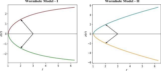
Figure 1. Two-dimensional graphic representation of embedding diagrams of wormhole w.r.t SF-1 (left) and w.r.t SF-2 (right).
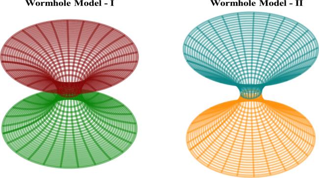
Figure 2. Wormhole surface diagram w.r.t SF-1 (left) and w.r.t SF-2 (right)
Figure 3. Attributes of SF-1 with r0 = 1 and δ = 0.5
In ${ \mathcal F }({ \mathcal R },{{\mathscr{L}}}_{m})$ gravity, γ acts as a coupling between particle and field of gravitation. We have found that the criteria of positive energy density restricts the arbitrariness of γ and it leads to γ ≥ 5. Eventually, one can get the same qualitative outcomes for the physical features of the model for any range of γ provided γ ≥ 5. So, to analyse the effects of coupling on the WH configuration, we have taken a small range γ ∈ [5, 10] for two models of WHs in our study.
For SF-1, the energy density was positive throughout the spacetime. The behavior of the energy conditions is observed through graphs. It can be noted that from figure 4, for γ ∈ [5, 10], the radial NEC is found to be violated throughout the entire range of r ≥ 1. While the tangential NEC is violated only in a small range 1.363 < r < 1.8 and satisfied otherwise. In addition, SEC is violated within γ ∈ [5, 10] throughout the radial coordinate r (figure 4, right bottom panel). Also, the radial DEC is violated within γ ∈ [5, 10] for the entire range of r ≥ 1, while tangential DEC ($\rho -| {{ \mathcal P }}_{t}| $) is satisfied for 1 ≤ r < 1.366 and violated for 1.366 < r < 1.8 with respective to SF-1. Furthermore, for r ≥ 1.8, $\rho -| {{ \mathcal P }}_{t}| \leqslant 0$ . Ultimately, we created table 1 which compiles all our findings. The violation of WEC and NEC occurred due to the effective energy-momentum tensor and becomes a source for the exotic matter to support the WH solutions in figure 5.
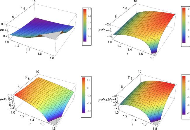
Figure 4. Behavior of ρ (top left panel), $\rho +{{ \mathcal P }}_{r}$ (top right panel), $\rho +{{ \mathcal P }}_{t}$ (bottom left panel), and $\rho +{{ \mathcal P }}_{r}+2{{ \mathcal P }}_{t}$ (right bottom panel) with δ = 0.5, γ ∈ [5, 10] and r0 = 1 for WH-I .
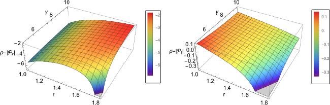
Figure 5. Behavior of $\rho -| {{ \mathcal P }}_{r}| $ (left panel) and $\rho -| {{ \mathcal P }}_{t}| $ (right panel) with δ = 0.5, γ ∈ [5, 10] and r0 = 1 for WH-I.
Table 1. Aspects of different strategies with execution of physical expressions for both cases.
Strategy Physical Expressions Interpretation
SF-1: ρ >0 for r ≥ 1
${N}_{{ \mathcal S }}(r)={r}_{0}{\left(\tfrac{\cosh ({r}_{0})}{\cosh (r)}\right)}^{\delta }$, δ > 0 $\rho +{{ \mathcal P }}_{r}$ <0 for r ≥ 1
Parameters $\rho +{{ \mathcal P }}_{t}$ >0 for 1 ≤ r < 1.368,
γ ∈ [5, 10], <0 for 1.368 < r < 1.8 &
r0 = 1 & δ = 0.5 ≥0 for r ≥ 1.8
$\rho -| {{ \mathcal P }}_{r}| $ <0 for r ≥ 1
$\rho -| {{ \mathcal P }}_{t}| $ >0 for 1 ≤ r < 1.366,
<0 for 1.366 < r < 1.8 &
≤0 for r ≥ 1.8
$\rho +{{ \mathcal P }}_{r}+2{{ \mathcal P }}_{t}$ <0 for r ≥ 1
${N}_{{ \mathcal S }}(r)$ ${N}_{{ \mathcal S }}(r)\gt 0$ w.r.t radial coordinate r
${N}_{{ \mathcal S }}(r)$ ${N}_{{ \mathcal S }}(r)-r\,=\,0$ with r0 = 1.
${N}_{{ \mathcal S }}^{{\prime} }(r)$ ${N}_{{ \mathcal S }}^{{\prime} }\lt 1$ when rr0.
$\tfrac{{N}_{{ \mathcal S }}(r)}{r}$ $\tfrac{{N}_{{ \mathcal S }}(r)}{r}\to 0$ as r → ∞ .
${{\mathscr{F}}}_{{hf}}+{{\mathscr{F}}}_{{gf}}+{{\mathscr{F}}}_{{af}}=0$ Satisfied .
${ \mathcal V }{ \mathcal I }{ \mathcal Q }=8\pi {\int }_{{r}_{0}}^{{r}_{1}}(\rho +{{ \mathcal P }}_{r}){r}^{2}{\rm{d}}r$ ${ \mathcal V }{ \mathcal I }{ \mathcal Q }\to 0$ as r1r0.

SF-2: ρ >0 for r ≥ 1
${N}_{{ \mathcal S }}(r)=\tfrac{1}{r}+\mathrm{log}\left(\tfrac{r}{{r}_{0}}\right)$. $\rho +{{ \mathcal P }}_{r}$ <0 for r ≥ 1
Parameters $\rho +{{ \mathcal P }}_{t}$ >0 for 1 ≤ r < 1.364 &
<0 for r ≥ 1.364
γ ∈ [5, 10] & r0 = 1. $\rho -| {{ \mathcal P }}_{r}| $ <0 for r ≥ 1
$\rho -| {{ \mathcal P }}_{t}| $ >0 for 1 ≤ r < 1.366 &
<0 for r ≥ 1.366
$\rho +{{ \mathcal P }}_{r}+2{{ \mathcal P }}_{t}$ <0 for r ≥ 1
${N}_{{ \mathcal S }}(r)$ ${N}_{{ \mathcal S }}(r)\gt 0$ w.r.t radial coordinate r
${N}_{{ \mathcal S }}(r)-r$ ${N}_{{ \mathcal S }}(r)(r)-r\,=\,0$ with r0 = 1.
${N}_{{ \mathcal S }}^{{\prime} }(r)$ ${N}_{{ \mathcal S }}^{{\prime} }\lt 1$ when rr0.
$\tfrac{{N}_{{ \mathcal S }}(r)}{r}$ $\tfrac{{N}_{{ \mathcal S }}(r)}{r}\to 0$ as r → ∞ .
${{\mathscr{F}}}_{{hf}}+{{\mathscr{F}}}_{{gf}}+{{\mathscr{F}}}_{{af}}=0$ Satisfied.
${ \mathcal V }{ \mathcal I }{ \mathcal Q }=8\pi {\int }_{{r}_{0}}^{{r}_{1}}(\rho +{{ \mathcal P }}_{r}){r}^{2}{\rm{d}}r$ ${ \mathcal V }{ \mathcal I }{ \mathcal Q }\to 0$ as r1r0.

6.2. Wormhole model—II

Now, we define another shape function-2 (SF-2) given by
$\begin{eqnarray}{N}_{{ \mathcal S }}(r)=\displaystyle \frac{1}{r}+\mathrm{log}\left(\displaystyle \frac{r}{{r}_{0}}\right),\end{eqnarray}$
where this particular SF-2 with r0 = 1 satisfies all the required conditions for the shape of the WH.
From figure 6 it can be observed that the ${N}_{{ \mathcal S }}(r)-r$ cuts r-axis at r0 = 1. The asymptotic flatness $\tfrac{{N}_{{ \mathcal S }}(r)}{r}\to 0$ is confirmed as r → ∞ . Also, flare-out condition ${N}_{{ \mathcal S }}({r}_{0})\lt 1$, r > r0 is well achieved. The characteristics of the SF-2 are given in figure 6. The embedded surface diagram w.r.t SF-2 is shown in right panels of figure 1 and figure 2.
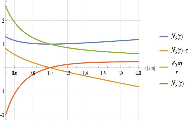
Figure 6. Characteristics of SF-2 with r0 = 1
The expressions for energy density, radial pressure, and tangential pressure under constant redshift function for SF-2 is given by
$\begin{eqnarray}\begin{array}{l}\rho =\displaystyle \frac{r-1}{{r}^{4}-2\gamma +2r\gamma },\end{array}\end{eqnarray}$
$\begin{eqnarray}\begin{array}{l}{{ \mathcal P }}_{r}=-\displaystyle \frac{1}{{r}^{3}({r}^{4}-2\gamma -2r\gamma )}\left(2({r}^{4}-6\gamma +8r\gamma -2{r}^{2}\gamma \right.\\ \left.+r({r}^{4}-4\gamma +4r\gamma )\mathrm{log}(\displaystyle \frac{r}{{r}_{0}}))\right),\end{array}\end{eqnarray}$
$\begin{eqnarray}{{ \mathcal P }}_{t}=-\displaystyle \frac{(r-1)({r}^{2}-1)}{r({r}^{4}-2\gamma +2r\gamma )}.\end{eqnarray}$
Similarly, with the help of equations (34)–(36), the radial NEC and tangential NEC, DEC, and SEC are given by,
$\begin{eqnarray}\begin{array}{l}\rho +{{ \mathcal P }}_{r}=-\displaystyle \frac{1}{{r}^{3}({r}^{4}-2\gamma +2r\gamma )}2\left(\Space{0ex}{2.5ex}{0ex}{r}^{3}-6\gamma +8r\gamma -2{r}^{2}\gamma \right.\\ \left.+r({r}^{4}-4\gamma -4r\gamma )\mathrm{log}(\displaystyle \frac{r}{{r}_{0}})\right),\end{array}\end{eqnarray}$
$\begin{eqnarray}\begin{array}{l}\rho +{{ \mathcal P }}_{t}=-\displaystyle \frac{1+r-4{r}^{2}+2{r}^{3}}{{r}^{5}-2r\gamma +2{r}^{2}\gamma }.\end{array}\end{eqnarray}$
$\begin{eqnarray}\begin{array}{l}\rho -| {{ \mathcal P }}_{r}| =\displaystyle \frac{2(r-1)}{{r}^{4}-2\gamma +2r\gamma }-\left|-\displaystyle \frac{1}{{r}^{3}({r}^{4}-2\gamma -2r\gamma )}\right.\\ \times \left(2\left\{{r}^{4}-6\gamma +8r\gamma -2{r}^{2}\gamma +r({r}^{4}-4\gamma +4r\gamma )\right.\right.\\ \left.\left.\left.\times \mathrm{log}\left(\displaystyle \frac{r}{{r}_{0}}\right)\right\}\right)\right|,\end{array}\end{eqnarray}$
$\begin{eqnarray}\begin{array}{l}\rho -| {{ \mathcal P }}_{t}| =\displaystyle \frac{2(r-1)}{{r}^{4}-2\gamma +2r\gamma }-\left|-\displaystyle \frac{(r-1)({r}^{2}-1)}{r({r}^{4}-2\gamma +2r\gamma )}\right|,\end{array}\end{eqnarray}$
$\begin{eqnarray}\begin{array}{l}\rho +{{ \mathcal P }}_{r}+2{{ \mathcal P }}_{t}=-\displaystyle \frac{1}{{r}^{3}({r}^{4}-2\gamma +2r\gamma )}2\left({r}^{3}-6\gamma +8r\gamma \right.\\ -2{r}^{2}\gamma +r({r}^{4}-4\gamma -4r\gamma )\mathrm{log}\left(\displaystyle \frac{r}{{r}_{0}}\right)\\ -\left.2\displaystyle \frac{(r-1)({r}^{2}-1)}{r({r}^{4}-2\gamma +2r\gamma )}\right).\end{array}\end{eqnarray}$
With SF-2, we analyzed the behavior of all ECs with model parameter γ. We set the free parameter as γ ∈ [5, 10]. The energy density shows positive behavior throughout the spacetime figure 7 (top left panel). With this range of γ, the radial NEC shows negative behavior for r ≥ 1. The tangential NEC is satisfied for 1 ≤ r < 1.364 and violated for of r ≥ 1.364. The development of radial DEC suggests that it shows negative behavior throughout the entire range of r ≥ 1 while tangential DEC violated for r ≥ 1.366, and is satisfied for 1 ≤ r < 1.366. Additionally, the SEC is violated for r ≥ 1. The behavior of the ECs above can be seen in figures 7- 8. At last, we summarized our results in table 1. The effective energy-momentum tensor caused the violation of the WEC and acts as a source of exotic matter to sustain the WH solutions.
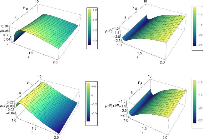
Figure 7. Behavior of ρ (top left panel), $\rho +{{ \mathcal P }}_{r}$ (top right panel), $\rho +{{ \mathcal P }}_{r}$ (bottom left panel), and $\rho +{{ \mathcal P }}_{r}+2{{ \mathcal P }}_{t}$ (right bottom panel) with γ ∈ [5, 10] and r0 = 1 for WH-II.
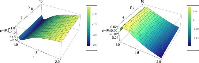
Figure 8. Behavior of $\rho -| {{ \mathcal P }}_{r}| $ (left panel) and $\rho -| {{ \mathcal P }}_{t}| $ (right panel) with γ ∈ [5, 10] and r0 = 1 for WH-II.

7. Equilibrium condition

It is important to determine the equilibrium configuration of a WH is stable or unstable. So, we will introduce the equilibrium condition of the presented WH models within ${ \mathcal F }({ \mathcal R },{{\mathscr{L}}}_{m})$ gravity.
The TOV equation [63] for an anisotropic configuration is expressed as
$\begin{eqnarray}\displaystyle \frac{{\rm{d}}{{ \mathcal P }}_{r}}{{\rm{d}}r}+\displaystyle \frac{{\kappa }^{{\prime} }(r)({{ \mathcal P }}_{r}+\rho )}{2}+\displaystyle \frac{2({{ \mathcal P }}_{r}-{{ \mathcal P }}_{t})}{r}=0,\end{eqnarray}$
where κ(r) = 2 × ζ(r) and ζ(r) denotes redshift function which is a function of radial coordinate ‘r’.
Here equation (42) gives the depiction of the equilibrium of a WH under three types of forces defined below:

${{\mathscr{F}}}_{{\bf{gf}}}$: The force of gravity produced by gravitating mass.

${{\mathscr{F}}}_{{\bf{af}}}$: An anisotropic force is produced by the anisotropy of the system.

${{\mathscr{F}}}_{{\bf{hf}}}$: Hydrostatic fluid generates hydrostatic force.

Such forces can be expressed as:

${{\mathscr{F}}}_{{gf}}=\tfrac{-{\kappa }^{{\prime} }(r)({{ \mathcal P }}_{r}+\rho )}{2}$.

${{\mathscr{F}}}_{{af}}=\tfrac{2({{ \mathcal P }}_{t}-{{ \mathcal P }}_{r})}{r}$.

${{\mathscr{F}}}_{{hf}}=-\tfrac{{\rm{d}}{{ \mathcal P }}_{r}}{{\rm{d}}r}$.

Since ${{\mathscr{F}}}_{{hf}}+{{\mathscr{F}}}_{{gf}}+{{\mathscr{F}}}_{{af}}=0$, counterpoise for WH solution to be in stable equilibrium.
The expression for ${{\mathscr{F}}}_{{hf}}$ and ${{\mathscr{F}}}_{{af}}$ w.r.t to SF-1 are mentioned below:
$\begin{eqnarray}\begin{array}{l}{{\mathscr{F}}}_{{hf}}=-\displaystyle \frac{1}{({r}^{3}{\left({r}^{2}-2{r}_{0}\delta \gamma {\left(\cosh ({r}_{0}){\rm{sech}} (r)\right)}^{\delta }\tanh (r)\right)}^{2})}\\ \times \left((4\delta ({r}^{4}-8{r}_{0}^{2}{r}^{2}\gamma {\left(\cosh ({r}_{0}){\rm{sech}} (r)\right)}^{2\delta }\tanh (r)\right.\\ +{r}_{0}\delta \gamma {\left(\cosh ({r}_{0}){\rm{sech}} (r)\right)}^{\delta }\\ \times (\delta {r}^{3}+{r}_{0}{\left(\cosh ({r}_{0}){\rm{sech}} (r)\right)}^{\delta }(-7{r}^{3}\\ +8{r}_{0}\gamma {\left(\cosh ({r}_{0}){\rm{sech}} (r)\right)}^{\delta })\tanh {\left(r\right)}^{2}\\ +2{r}_{0}^{2}{\delta }^{2}r\gamma {\left(\cosh ({r}_{0}){\rm{sech}} (r)\right)}^{2\delta }\\ (-{r}^{3}+3{r}_{0}\gamma {\left(\cosh ({r}_{0}){\rm{sech}} (r)\right)}^{\delta }\tanh {\left(r\right)}^{3}\\ +2{r}_{0}^{3}{\delta }^{3}{r}^{2}{\gamma }^{2}{\left(\cosh ({r}_{0}){\rm{sech}} (r)\right)}^{3\delta }\tanh {\left(r\right)}^{4}\\ -{r}_{0}{r}^{2}\gamma {\rm{sech}} {\left(r\right)}^{2}\left(\cosh ({r}_{0})\right.\\ {\left.{\rm{sech}} (r)\right)}^{\delta }(r(\delta -2{r}_{0}{\left(\cosh ({r}_{0}){\rm{sech}} (r)\right)}^{\delta })\\ -2{r}_{0}\delta {r}^{2}{\left(\cosh ({r}_{0}){\rm{sech}} (r)\right)}^{\delta }\tanh (r)\\ \left.+2{r}_{0}^{2}{\delta }^{2}\gamma {\left(\cosh ({r}_{0}){\rm{sech}} (r)\right)}^{2\delta }\tanh {\left(r\right)}^{2}))))\right),\end{array}\end{eqnarray}$
$\begin{eqnarray}\begin{array}{l}{{\mathscr{F}}}_{{af}}=\displaystyle \frac{1}{-{r}^{5}-2{r}_{0}\delta {r}^{3}\gamma {\left(\cosh ({r}_{0}){\rm{sech}} (r)\right)}^{\delta }\tanh (r)}\\ \times \left((2\delta (-2{r}^{2}+{r}_{0}{\left(\cosh ({r}_{0}){\rm{sech}} (r)\right)}^{\delta }(r-2{r}^{3}\right.\\ +8{r}_{0}\gamma {\left(\cosh ({r}_{0}){\rm{sech}} (r)\right)}^{\delta })\tanh (r)\\ \left.-4{r}_{0}^{2}\delta r\gamma {\left(\cosh ({r}_{0}){\rm{sech}} (r)\right)}^{2\delta }\tanh {\left(r\right)}^{2}\right).\end{array}\end{eqnarray}$
Similarly w.r.t SF-2, ${{\mathscr{F}}}_{{hf}}$ and ${{\mathscr{F}}}_{{af}}$ is given by,
$\begin{eqnarray}\begin{array}{l}{{\mathscr{F}}}_{{hf}}=\displaystyle \frac{1}{{r}^{4}{\left({r}^{4}-2\gamma +2r\gamma \right)}^{2}}\\ \times \ 2\left(3{r}^{8}-{r}^{9}-40{r}^{4}\gamma +54{r}^{5}\gamma \right.\\ -16{r}^{6}\gamma +36{\gamma }^{2}-88r{\gamma }^{2}\\ +\ 68{r}^{2}{\gamma }^{2}-16{r}^{3}{\gamma }^{2}\\ +\ 2r({r}^{8}-10{r}^{4}\gamma +9{r}^{5}\gamma +8{\gamma }^{2}\\ \left.-16r{\gamma }^{2}+8{r}^{2}{\gamma }^{2})\mathrm{log}(\displaystyle \frac{r}{{r}_{0}})\right),\end{array}\end{eqnarray}$
$\begin{eqnarray}\begin{array}{l}{{\mathscr{F}}}_{{af}}=\displaystyle \frac{1}{{r}^{4}({r}^{4}-2\gamma +2r\gamma )}\\ \times 2\left({r}^{3}+4{r}^{4}-2{r}^{5}-12\gamma \right.\\ +16r\gamma -{r}^{2}(1+4\gamma )\\ \left.+2r({r}^{4}-4\gamma +4r\gamma )\mathrm{log}(\displaystyle \frac{r}{{r}_{0}})\right).\end{array}\end{eqnarray}$
We have made an analysis of the WH solution’s stability with features of ${{\mathscr{F}}}_{{hf}}$, ${{\mathscr{F}}}_{{af}}$ and ${{\mathscr{F}}}_{{gf}}$ acting on the WH in the current scenario. The effect of ${{\mathscr{F}}}_{{gf}}$, the gravitational force is null as we take the redshift function constant. One can observe from figure 9 that the graphical behavior of these forces is in equilibrium. The hydrostatic force (${{\mathscr{F}}}_{{hf}}$) is balanced by the anisotropic force (${{\mathscr{F}}}_{{af}}$). Therefore, our current models w.r.t SF-1 and SF-2 are in stable equilibrium.
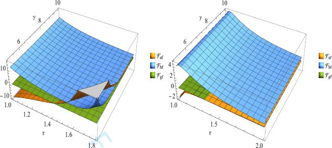
Figure 9. Equilibrium scenario via TOV equation with r0 = 1 and δ = 0.5 for SF-1 (left panel) and for SF-2 with r0 = 1 (right panel)

8. Volume integral quantifier

We will now make an estimation of the volume of exotic material needed for a stable WH. Visser et al [64] introduced the method to determine the volume integral quantifier (${ \mathcal V }{ \mathcal I }{ \mathcal Q }$) which is given by
$\begin{eqnarray}{ \mathcal V }{ \mathcal I }{ \mathcal Q }=\oint (\rho +{{ \mathcal P }}_{r}){\rm{d}}{ \mathcal V },\end{eqnarray}$
where, ${\rm{d}}{ \mathcal V }={r}^{2}{\rm{d}}r{\rm{d}}{\rm{\Psi }}$. Since $\oint {\rm{d}}{ \mathcal V }=2{\int }_{{r}_{0}}^{\infty }{\rm{d}}{ \mathcal V }=8\pi {\int }_{{r}_{0}}^{\infty }{r}^{2}{\rm{d}}r$, we have
$\begin{eqnarray}{ \mathcal V }{ \mathcal I }{ \mathcal Q }=8\pi {\int }_{{r}_{0}}^{\infty }(\rho +{{ \mathcal P }}_{r}){r}^{2}{\rm{d}}r.\end{eqnarray}$
Here ${ \mathcal V }{ \mathcal I }{ \mathcal Q }$ corresponding to WH that varies from r0 to r1 such that r1r0 and defined as
$\begin{eqnarray}{ \mathcal V }{ \mathcal I }{ \mathcal Q }=8\pi {\int }_{{r}_{0}}^{{r}_{1}}(\rho +{{ \mathcal P }}_{r}){r}^{2}{\rm{d}}r.\end{eqnarray}$
With equation (49), we investigated the ${ \mathcal V }{ \mathcal I }{ \mathcal Q }$ and provide the graphical scenario in figure 10. It can be observed that ${ \mathcal V }{ \mathcal I }{ \mathcal Q }$ is negative for r > r0 implying the presence of exotic matter for both the WH models. However, if one approaches near the throat, the amount of exotic matter reduces significantly as ${ \mathcal V }{ \mathcal I }{ \mathcal Q }\to 0$ as r1r0. As a result, we can say that just a small amount of exotic matter can maintain a WH configuration near the throat for both models. By choosing an appropriate WH geometry, we discovered that reducing the amount of exotic matter that violates the averaged null energy condition (ANEC) is possible. For further details, one can also go with these references [65, 66].
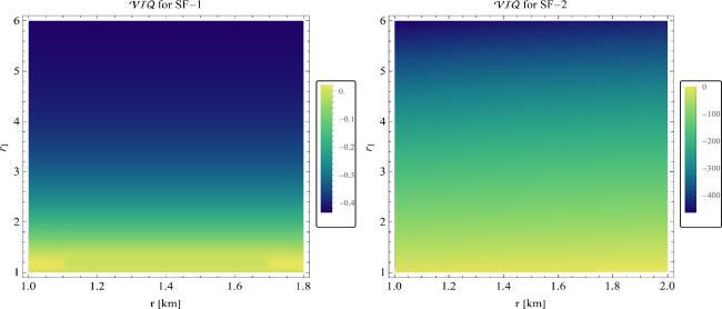
Figure 10. ${ \mathcal V }{ \mathcal I }{ \mathcal Q }$ with r0 = 1, δ = 0.5 and γ = 5 - SF-1 (left panel) and with r0 = 1, γ = 5 -SF-2 (right panel)

9. Concluding remarks

In the present work, we have developed an interest in WH solutions within the context of modified gravity theories. In order to create WHs without the need for undiscovered exotic matter, modified gravity theories are crucial. In this work, we have investigated different WH solutions in ${ \mathcal F }({ \mathcal R },{{\mathscr{L}}}_{m})$ modified gravity utilizing two different shape functions, SF-1 and SF-2 given in equations (24) and (33), respectively. The results of the presented model will be put forward in the discussion provided below:
i

(i) The investigation is initiated by showing in figures 3 and 6 that SF-1 and SF-2 fulfill all the physical criteria for the construction of a WH. Following that, graphical representations of embedding surfaces have been shown for both the models of WHs in figures 1 and 2.

ii

(ii) We proceeded to the investigation by analyzing the energy conditions viz. NEC, DEC, and SEC respectively for both the models. With respect to SF-1, taking r0 = 1, 5 ≤ γ ≤ 10 and δ = 0.5, we found in figures 4 and 5 that the radial NEC is completely violated and the tangential NEC is violated within the mentioned range of γ and r while DEC and SEC also violated. On the other hand, we analyzed the characteristics of all ECs with model parameter 5 ≤ γ ≤ 10 with respect to SF-2 and found that the energy density shows positive behavior throughout the spacetime figure 7 (top left panel). With different ranges of r, the radial NEC, and radial DEC, as well as the SEC, are violated with 5 ≤ γ ≤ 10, as can be seen in figures 7 and 8. The effective energy-momentum tensor caused the violation of the WEC and turned into a source of exotic matter to support the WH solutions.

iii

(iii) Keeping in mind the above results, we continued the exploration regarding the stability analysis of the two WH models. For this, the equilibrium condition of the presented WH models within ${ \mathcal F }({ \mathcal R },{{\mathscr{L}}}_{m})$ gravity is introduced by the TOV equation [63] for an anisotropic configuration. This is realized as the stability of a WH is featured by three forces such as ${{\mathscr{F}}}_{{hf}}$, ${{\mathscr{F}}}_{{af}}$ and ${{\mathscr{F}}}_{{gf}}$. In the current scenario, ${{\mathscr{F}}}_{{gf}}$ has zero effect on the WH as the redshift function is constant. Figure 9 confirms that the anisotropic force (${{\mathscr{F}}}_{{af}}$) balances the hydrostatic force (${{\mathscr{F}}}_{{hf}}$). Hence, the graphical behavior of these forces shows that the WH models w.r.t SF-1 and SF-2 are in stable equilibrium.

iv

(iv) The quest for minimal presence of exotic matter in a WH in the framework of ${ \mathcal F }({ \mathcal R },{{\mathscr{L}}}_{m})$ drove the present study to determine volume integral quantifier. Additionally, we looked at the ${ \mathcal V }{ \mathcal I }{ \mathcal Q }$ to investigate how much exotic material is needed at the neck to create a traversable WH. We provided the graphical scenario of ${ \mathcal V }{ \mathcal I }{ \mathcal Q }$ for both SF-1 and SF-2 in figure 10. Exotic matter is present in both the WH models as it can be seen that ${ \mathcal V }{ \mathcal I }{ \mathcal Q }$ is negative for r > r0. However, near the throat, the amount of exotic matter decreases considerably as ${ \mathcal V }{ \mathcal I }{ \mathcal Q }\to 0$ as r1r0. This leads to the result that just a small amount of exotic matter can sustain a WH configuration near the throat for both models.

v

(v) Now, we will present some relevant research works on WHs in different modified theories of gravity in connection to our present work. In a power law f(T) model [50], WH solutions considering energy density to be Gaussian violate radial NEC in some region of spacetime whereas tangential NEC is valid everywhere. Later, with the assumption of linear equation of states, a dynamical model [51] in f(T) gravity for WH follows the violation of NEC with some evolving time constraint. Another the investigation [52] of WH solutions in Finsler geometry establishes violation of radial NEC for the chosen and physically valid shape functions. Further, NEC in radial direction is not satisfied but valid in a tangential direction for specific equation of state taken into account in the framework of f(R, T) gravity [53]. A similar exploration related to NEC can be found in research works [54, 55] on WHs in f(R) gravity where physically valid shape functions are taken into consideration. Again, similar results for WH solutions are obtained in a linear model under f(Q, T) gravity [56] with Gaussian and Lorentzian distribution profiles of density. In the same work [56], a non linear model for WHs shows that radial NEC fails to satisfy only near the throat. In the background of Rastall gravity, Chaudhary et al [57] developed WH configurations by utilizing various linear equations of state and showed that exotic matter is required in accordance to violation of radial NEC. Recently, Kavya et al [58] showed the behavior of ECs in the context of ${ \mathcal F }({ \mathcal R },{{\mathscr{L}}}_{m})$ by using specific forms of energy density and shape functions to produce physically viable WH solutions. In their work, NEC was found to be violated for WH model A, whereas it is satisfied for model B. Again, Solanki et al [59] provide the WH solutions in ${ \mathcal F }({ \mathcal R },{{\mathscr{L}}}_{m})$ with different equations of states and specific forms of shape function to generate WH solutions. So, the expedition to explore WH geometries under modified theories of gravity continues in our present work. We have used a similar approach to the ones used in [52, 54, 55, 60] to develop two WH models in ${ \mathcal F }({ \mathcal R },{{\mathscr{L}}}_{m})$ gravity. For both the models, the energy density ρ is positive throughout the spacetime and NEC in the radial direction is violated. This result behaves as the key feature for a stable traversable WH in GR, as well as in alternative gravities [5058]. However, from the perspective of $f({ \mathcal Q })$ gravity, Kiroriwal et al [60] produced WH geometries by assuming physical form of shape functions which violates NEC in a tangential direction only. In contrast to the works [50, 5356], NEC in a tangential direction is violated only for some specified region near the throat of the WH for the WH-I model. However, tangential NEC is satisfied only near the throat of the WH for the WH-II model. In comparison to [58] and [59], we provide the stability of WHs for the WH-I and WH-II, along with the behavior of different forces acting on fluid via the dynamics of TOV equation.

Thus, in our work, we provide the WH solution by two newly developed shape functions in equations (24) and (33). It is important to note that the results of the current investigation in the background of ${ \mathcal F }({ \mathcal R },{{\mathscr{L}}}_{m})$ gravity are physically possible. All our results are compatible and support the analysis of existing results in modified ${ \mathcal F }({ \mathcal R },{{\mathscr{L}}}_{m})$ gravity .

Conflict of Interest Statement

The authors declare that they have no conflicts of interest or personal relationships that could have appeared to influence the work reported in this paper.

S K Maurya and A Aziz appreciate the administration of the University of Nizwa in the Sultanate of Oman for their unwavering support and encouragement. S Chaudhary expresses his gratitude to the Central University of Haryana for providing a University Research Fellowship (URF) under the Reg. No. 222019. J Kumar is highly thankful to the Department of Mathematics, Central University of Haryana. S Kiroriwal acknowledges the University Grant Commission (UGC), New Delhi, India under the NTA Ref. No. 211610000030 for providing financial support.

1
Schwarzschild K 1916 On the Gravitational Field of a Mass Point according to Einstein’s Theory Sitzungsber. Preuss. Akad. Wiss. Berlin (Math. Phys.) 1916 189 196 arXiv preprint physics/9905030

2
Schwarzschild K 2003 “Golden Oldie”: On the Gravitational Field of a Mass Point According to Einstein's Theory General Relativity and Gravitation 35 5 951 959

3
Einstein A 1917 Sitzungsber. Preuss. Akad. Wiss. New York Dover 177 English translation in The Principle of Relativity

4
Flamm L 2015 Republication of: Contributions to Einstein’s Theory of Gravitation Gen. Relativ. Gravit. 47 72

DOI

5
Einstein A, Rosen N 1935 The particle problem in the general theory of relativity Phys. Rev. 48 73 77

DOI

6
Morris M S, Thorne K S 1988 Wormholes in spacetime and their use for interstellar travel: A tool for teaching general relativity Am. J. Phys. 56 395 412

DOI

7
Nicolis A, Rattazzi R, Trincherini E 2010 Energy’s and amplitudes positivity J. High Energy Phys. JHEP05(2010)095

DOI

8
Kallosh R, Linde A, Linde D, Susskind L 1995 Gravity and global symmetries Phys. Rev. D 52 912 935

DOI

9
Hayward S A 1999 Dynamic wormholes Int. J. Mod. Phys. D 8 373 382

DOI

10
Lobo F S 2006 Chaplygin traversable wormholes Phys. Rev. D 73 064028

DOI

11
Perry G P, Mann R B 1992 Traversible wormholes in (2. 1) dimensions Gen. Rel. Grav. 24 305 321

DOI

12
Fuller R W, Wheeler J A 1962 Causality and multiply connected space-time Phys. Rev. 128 919 929

DOI

13
Morris M S, Thorne K S, Yurtsever U 1988 Wormholes, time machines, and the weak energy condition Phys. Rev. Lett. 61 1446 1449

DOI

14
Israel W 1966 Singular hypersurfaces and thin shells in general relativity Nuovo Cim. 44S10 1

DOI

15
Eiroa E F, Simeone C 2004 Cylindrical thin-shell wormholes Phys. Rev. D 70 044008

DOI

16
Lobo F S, Crawford P 2003 Linearized stability analysis of thin-shell wormholes with a cosmological constant Class. Quant. Grav. 21 391 404

DOI

17
Lobo F S, Crawford P 2005 Stability analysis of dynamic thin shells Class. Quant. Grav. 22 4869 4886

DOI

18
Lemos J P, Lobo F S 2008 Plane symmetric thin-shell wormholes: Solutions and stability Phys. Rev. D 78 044030

DOI

19
Eiroa E F, Simeone C 2010 Some general aspects of thin-shell wormholes with cylindrical symmetry Phys. Rev. D 81 084022

DOI

20
Eiroa E F, Simeone C 2010 Brans-Dicke cylindrical wormholes Phys. Rev. D 82 084039

DOI

21
Anchordoqui L A, Bergliaffa S P, Torres D F 1997 Brans-Dicke wormholes in nonvacuum spacetime Phys. Rev. D 55 5226 5229

DOI

22
Anchordoqui L A, Bergliaffa S E P 2000 Wormhole surgery and cosmology on the brane: The world is not enough Phys. Rev. D 62 067502

DOI

23
Nandi K K, Bhattacharjee B, Alam S M K, Evans J 1998 Brans-Dicke wormholes in the Jordan and Einstein frames Phys. Rev. D 57 823 828

DOI

24
Godani N, Samanta G C 2020 Traversable wormholes in R + αRn gravity Eur. Phys. J. C 80 30 Traversable wormholes in R+αRn gravity

DOI

25
Godani N, Samanta G C 2019 Traversable wormholes and energy conditions with two different shape functions in f (R) gravity Int. J. Mod. Phys. D 28 1950039

DOI

26
Furey N, DeBenedictis A 2004 Wormhole throats in Rm gravity Class. Quant. Grav. 22 313 322

DOI

27
Mehdizadeh M R, Ziaie A H 2017 Einstein-Cartan wormhole solutions Phys. Rev. D 95 064049

DOI

28
Errehymy A, Hansraj S, Maurya S K, Hansraj C, Daoud M 2023 Spherically symmetric traversable wormholes in the torsion and matter coupling gravity formalism Phys. Dark Univ. 41 101258

DOI

29
Chakraborty K, Aziz A, Rahaman F, Ray S 2023 Quark matter supported wormhole in third order Lovelock gravity Chin. J. Phys. 83 315 324

DOI

30
Klinkhamer F R 2023 New Type of Traversable Wormhole arXiv:2307.04678

31
Capozziello S, De Laurentis M 2011 Extended theories of gravity Phys. Rept. 509 167 321

DOI

32
Capozziello S, Lobo F S, Mimoso J P 2015 Generalized energy conditions in extended theories of gravity Phys. Rev. D 91 124019

DOI

33
Bronnikov K A, Grinyok S 2002 Instability of wormholes with a nonminimally coupled scalar field Grav. Cosmol. 7 297 300

34
Bronnikov K A, Starobinsky A A 2007 No realistic wormholes from ghost-free scalar-tensor phantom dark energy JETP Lett. 85 1 5

DOI

35
Gonzalez J A, Guzman F S, Sarbach O 2008 Instability of wormholes supported by a ghost scalar field: I. Linear stability analysis Class. Quant. Grav. 26 015010

DOI

36
Mustafa G, Maurya S K, Ray S 2022 On the possibility of generalized wormhole formation in the galactic halo due to dark matter using the observational data within the matter coupling gravity formalism Astrophys. J. 941 170

DOI

37
Mustafa G, Maurya S K, Ray S 2023 Relativistic wormhole surrounded by dark matter halos in symmetric teleparallel gravity Fortsch. Phys. 71 2200129

DOI

38
Bertolami O, Boehmer C G, Harko T, Lobo F S 2007 Extra force in f (R) modified theories of gravity Phys. Rev. D 75 104016

DOI

39
Harko T 2010 Galactic rotation curves in modified gravity with nonminimal coupling between matter and geometry Phys. Rev. D 81 084050

DOI

40
Harko T 2010 The matter Lagrangian and the energy-momentum tensor in modified gravity with nonminimal coupling between matter and geometry Phys. Rev. D 81 044021

DOI

41
Harko T 2014 Thermodynamic interpretation of the generalized gravity models with geometry-matter coupling Phys. Rev. D 90 044067

DOI

42
Faraoni V 2007 Viability criterion for modified gravity with an extra force Phys. Rev. D 76 127501

DOI

43
Harko T, Lobo F S 2010 f (R, L m) gravity Eur. Phys. J. C 70 373 379

DOI

44
Capozziello S, Harko T, Koivisto T S, Lobo F S, Olmo G J 2012 Wormholes supported by hybrid metric-Palatini gravity Phys. Rev. D 86 127504

DOI

45
2013 The Classical Theory of Fields Landau L D Amsterdam Elsevier Vol. 2

46
Hochberg D, Visser M 1998 Dynamic wormholes, antitrapped surfaces, and energy conditions Phys. Rev. D 58 044021

DOI

47
Hochberg D, Visser M 1998 Null energy condition in dynamic wormholes Phys. Rev. Lett. 81 746 749

DOI

48
Tahim M O, Landim R R, Almeida C A S 2009 Spacetime as a deformable solid Mod. Phys. Lett. A 24 1209 1217

49
Wang J, Liao K 2012 Energy conditions in f (R, Lm) gravity Class. Quant. Grav. 29 215016

DOI

50
Sharif M, Rani S 2013 Wormhole solutions in f (T) gravity with noncommutative geometry Phys. Rev. D 88 123501

DOI

51
Sharif M, Rani S 2013 Dynamical wormhole solutions in f (T) gravity Gen. Relativ. Gravitation 45 2389 2402

DOI

52
Rahaman F, Paul N, Banerjee A, De S S, Ray S, Usmani A A 2016 The Finslerian wormhole models Eur. Phys. J. C 76 1 9

DOI

53
Moraes P H R S, Sahoo P K 2017 Modeling wormholes in f (R, T) gravity Phys. Rev. D 96 044038

DOI

54
Mishra B 2021 Wormhole solutions in f (R) gravity Int. J. Mod. Phys. D 30 2150061

DOI

55
Mishra B, Agrawal A S, Tripathy S K, Ray S 2022 Traversable wormhole models in f (R) gravity Int. J. Mod. Phys. J 37 2250010

DOI

56
Tayde M, Hassan Z, Sahoo P K 2023 Existence of wormhole solutions in f (Q, T) gravity under non-commutative geometries Phys. Dark Univ. 42 101288

DOI

57
Chaudhary S, Maurya S K, Kumar J, Kiroriwal S, Aziz A 2023 Physical characteristics of wormhole geometries under different EoS in the context of Rastall gravity Chin. J. Phys. 86 578 589

DOI

58
Kavya N S, Venkatesha V, Mustafa G, Sahoo P K, Rashmi S D 2023 Static traversable wormhole solutions in f (R, ${{\mathscr{L}}}_{m}$) gravity Chin. J. Phys. 84 1 11

DOI

59
Solanki R, Hassan Z, Sahoo P K 2023 Wormhole solutions in f (R, Lm) gravity Chin. J. Phys. 85 74 88

DOI

60
Kiroriwal S, Kumar J, Maurya S K, Chaudhary S 2023 New spherically symmetric wormhole solutions in f (Q)-gravity theory Phys. Scr. 98 125305

DOI

61
Lobato R V, Carvalho G A, Bertulani C A 2021 Neutron stars in f(R, Lm) gravity with realistic equations of state: joint-constrains with GW170817, massive pulsars, and the PSR J0030. 0451 mass-radius from NICER data Eur. Phys. J. C 81 1013

DOI

62
Khoury J, Weltman A 2004 Chameleon fields: Awaiting surprises for tests of gravity in space Phys. Rev. Lett. 93 171104

DOI

63
Rahaman F, Kuhfittig P K F, Ray S, Islam N 2014 Possible existence of wormholes in the galactic halo region Eur. Phys. J. C 74 2750

DOI

64
Visser M, Kar S, Dadhich N 2003 Traversable wormholes with arbitrarily small energy condition violations Phys. Rev. Lett. 90 201102

DOI

65
Jusufi K, Channuie P, Jamil M 2020 Traversable wormholes supported by GUP corrected Casimir energy Eur. Phys. J. C 80 127

DOI

66
Sokoliuk O, Mandal S, Sahoo P K, Baransky A 2022 Generalised Ellis-Bronnikov wormholes in f (R) gravity Eur. Phys. J. C 82 280

DOI

Outlines

/