


1. Introduction
Ultracold atomic gases, due to the tunabilty of their interaction strength by Feshbach resonance (FR), provide an ideal platform for realizing different kinds of quantum phases [1–3]. In contrast to the widely studied s-wave FRs, the high partial wave FRs with nonzero relative angular momentum support various types of topological quantum matter such as topological superfluids and Majorana zero modes. In recent years, interacting quantum gases across p- and d-wave resonances have been realized and used to investigate the few-body and many-body problems in many experiments [4–15], and have also attracted some theoretical interest [16–20]. Some g-wave Feshbach resonances have also been studied in recent experiments [13, 21].
Spectroscopy is a powerful tool for investigating the rich many-body physics in ultracold quantum gases. Various spectroscopies are used in ultracold quantum gas experiments, for example radio-frequency (RF) spectroscopy, Bragg spectroscopy and lattice modulation spectroscopy [22, 23]. The RF spectral response of a unitary 6Li Fermi gas at different temperatures was observed in [24]. The RF response of impurities interacting with a quantum gas at finite temperature was investigated theoretically in [25, 26]. However, RF spectroscopy of high partial wave interacting quantum gases has rarely been studied.
Motivated by the recent experiments on high partial wave interacting quantum gases, we investigated the RF spectroscopy and momentum distribution of quantum Bose gases across p- and d-wave resonances in regions with different interaction strengths. The low-energy scattering amplitude can be characterized by the scattering volume vm (super-volume Dm) for p-wave (d-wave) interaction, the definition of which will be given in section 2 . In experiments, vm (Dm) can be tuned from negative to positive infinity by tuning the magnetic field [4, 14, 15], as illustrated schematically in figure 1. When vm > 0 (Dm > 0), there exists a shallow bound state with infinite lifetime, while for vm < 0 (Dm < 0) there is a quasi-bound state with positive binding energy due to the centrifugal barrier. As shown in figure 1, this quasi-bound state has a finite lifetime τ proportional to $1/{E}_{b}^{3/2}$ for p-waves ($1/{E}_{b}^{5/2}$ for d-waves) with Eb being the binding energy. The inverse lifetime 1/τ characterizes the coupling strength between the quasi-bound state and the scattering states, which have important influences in the RF spectrum. In analogy to the Bose–Einstein condensation (BEC)–Bardeen–Cooper–Schrieffer (BCS) crossover of fermions, we shall for convenience call the Eb < 0 region the BEC side and the Eb > 0 region the BCS side in this article.

Figure 1. Schematic of different interaction regions. The black solid lines show the scattering volume vm (super-volume Dm) as a function of magnetic field B, which diverges at resonance magnetic field ${B}_{\mathrm{res}}$. The red solid lines indicate the shallow bound state on the BEC side. On the BCS side, the red dashed lines indicate the quasi-bound state with positive binding energy and finite lifetime τ represented by the hatched area. |
We first introduce our two-channel model in section 2 . The self-energy of the single-particle Green’s function is obtained within the ladder diagram approximation or the so-called Nozières and Schmitt-Rink (NSR) scheme [19, 27]. In section 3 , the contact density is also derived within the NSR scheme through the adiabatic theorem [18, 28, 29], and is compared with the results from high-temperature virial expansion. Next, in section 4 , we present the results for the single-particle spectral function in which a clear anisotropic dependence in the momentum will be shown. The momentum distributions, obtained by integrating the single-particle spectral function over frequency, are analyzed in section 5 . Finally, results for the RF spectrum are presented and an estimation of signal strength (in terms of the atom transfer rate to final state) under typical experimental parameters are provided in section 6 .
2. Model
2.1. Hamiltonian
For strongly interacting Bose atoms across a p- or d-wave FR, the Hamiltonian can be written as the following two-channel model [19]:
$\begin{eqnarray}\begin{array}{l}{\hat{H}}_{0}=\displaystyle \sum _{{\boldsymbol{k}},\sigma ={\sigma }_{\mathrm{1,2}}}{\xi }_{{\boldsymbol{k}}}{\hat{a}}_{{\boldsymbol{k}},\sigma }^{\dagger }{\hat{a}}_{{\boldsymbol{k}},\sigma }+\displaystyle \sum _{{\boldsymbol{q}},m}\left({\xi }_{{\boldsymbol{q}},b}-{\nu }_{m}\right){\hat{b}}_{{\boldsymbol{q}},m}^{\dagger }{\hat{b}}_{{\boldsymbol{q}},m}\\ \quad +\sqrt{\displaystyle \frac{4\pi }{V}}\displaystyle \sum _{{\boldsymbol{k}},{\boldsymbol{q}},m}\left[{g}_{m}k{{\prime} }^{l}{Y}_{l,m}(\hat{{\boldsymbol{k}}}^{\prime} ){\hat{b}}_{{\boldsymbol{q}},m}^{\dagger }{\hat{a}}_{-{\boldsymbol{k}}+{\boldsymbol{q}},{\sigma }_{1}}{\hat{a}}_{{\boldsymbol{k}},{\sigma }_{2}}+{\rm{h}}.{\rm{c}}.\right],\end{array}\end{eqnarray}$
where ${\hat{a}}_{{\boldsymbol{k}},\sigma }$ and ${\hat{b}}_{{\boldsymbol{q}},m}$ are annihilation operators for atoms and closed-channel dimers and σ labels the different hyperfine states. The first and second terms correspond to the energy of free atoms and dimers. ${\xi }_{{\boldsymbol{k}}}=\tfrac{{{\hslash }}^{2}{k}^{2}}{2M}-\mu $ is the kinetic energy of an atom measured from its chemical potential μ. ${\xi }_{{\boldsymbol{q}},b}=\tfrac{{{\hslash }}^{2}{q}^{2}}{4M}-2\mu $ is the kinetic energy for a dimer measured from its chemical potential 2μ. To simplify the notation, we will set M = kB = ℏ = 1 (kB being the Boltzmann constant) throughout the rest of this paper. νm is the detuning for the m channel, with m standing for the magnetic quantum number. The last term in the Hamiltonian describes the coupling between the atom channel and the dimer channel with l = 1,2 corresponding to p- and d-wave resonances, respectively [4, 14, 15]. m = 0, ±1, ⋯ , ± l represent the quantum number of ${\hat{l}}_{z}$. ${\boldsymbol{k}}^{\prime} ={\boldsymbol{k}}-{\boldsymbol{q}}/2$ is the relative momentum of two incoming atoms that form the dimer and $k^{\prime} =| {\boldsymbol{k}}^{\prime} | $, $\hat{{\boldsymbol{k}}}^{\prime} ={\boldsymbol{k}}^{\prime} /k^{\prime} $. V is the volume of the system, gm is the strength of coupling and Yl,m(θ, φ) are the spherical harmonic functions.In this work, we consider a system very close to a certain p- or d-wave Feshbach resonance and far away from any other s-wave resonances. As a result, there are no low-energy s-wave bound states in the system under consideration. However, there will usually still be a small background s-wave scattering length abg in this region. In most cases, abg is of the same order as the van der Waals length, such that abgn1/3 ≪ 1 for a typical atom density n. We expect that the main effect of such a small residual s-wave interaction is to induce a meanfield shift of the chemical potential δμ ∼ 4πℏ2nabg/m, which does not change any of our results qualitatively. We thus believe that it should be a good approximation to neglect the s-wave interaction in this paper. Because the bosonic wave function must be symmetric under the exchange of two identical bosons, p-wave interaction can only exist between two different hyperfine states. As a result, for p-wave interaction we consider a two-components Bose gas where the summation of σ is over σ1,2 = 1, 2, while for d-wave interaction we consider a single-component Bose gas with σ1 = σ2 and the summation over σ drops out. In analogy to the Fermi gas, we will define a characteristic momentum unit kF as ${k}_{F}^{3}=3(6){\pi }^{2}{n}_{\mathrm{total}}$ for the two(single)-component Bose gas, and a corresponding energy unit ${E}_{F}={k}_{F}^{2}/2$. Here ntotal is the total particle number density of the Bose gas.
The bare parameters νm and gm are related to the low-energy scattering parameters through a set of renormalization relations [18–20]. For p-wave interaction, we have
$\begin{eqnarray}\displaystyle \frac{{\nu }_{m}}{{g}_{m}^{2}}=\displaystyle \frac{1}{4\pi }{v}_{p,m}^{-1}-\displaystyle \frac{1}{V}\displaystyle \sum _{{\boldsymbol{k}}}1,\end{eqnarray}$
$\begin{eqnarray}\displaystyle \frac{1}{{g}_{m}^{2}}=\displaystyle \frac{1}{4\pi }{R}_{p,m}^{-1}-\displaystyle \frac{1}{V}\displaystyle \sum _{{\boldsymbol{k}}}\displaystyle \frac{1}{{k}^{2}},\end{eqnarray}$
while for d-wave interaction, we have $\begin{eqnarray}\displaystyle \frac{{\nu }_{m}}{{g}_{m}^{2}}=\displaystyle \frac{1}{4\pi }{D}_{m}^{-1}-\displaystyle \frac{1}{V}\displaystyle \sum _{{\boldsymbol{k}}}{k}^{2},\end{eqnarray}$
$\begin{eqnarray}\displaystyle \frac{1}{{g}_{m}^{2}}=\displaystyle \frac{1}{4\pi }{v}_{d,m}^{-1}-\displaystyle \frac{1}{V}\displaystyle \sum _{{\boldsymbol{k}}}1,\end{eqnarray}$
$\begin{eqnarray}{R}_{d,m}^{-1}=\displaystyle \frac{4\pi }{V}\displaystyle \sum _{{\boldsymbol{k}}}\displaystyle \frac{1}{{k}^{2}},\end{eqnarray}$
where the meaning of the physical parameters Dm, vp(d),m and Rp(d),m will be clear in the two-particle vertex function presented in the next section.2.2. Self-energy
The self-energy of the single-particle Green’s function is obtained within the ladder diagram approximation as shown in figure 2 [19, 27]
$\begin{eqnarray}\begin{array}{l}{\rm{\Sigma }}({\boldsymbol{k}},{\rm{i}}{{\rm{\Omega }}}_{\nu })=-\displaystyle \frac{1}{\beta }\displaystyle \sum _{{\boldsymbol{q}}}\displaystyle \sum _{{\omega }_{n}}{\rm{\Gamma }}({\boldsymbol{q}},{\boldsymbol{k}}^{\prime} ,{\rm{i}}{\omega }_{n}){G}_{0}\\ \,\times \,(-{\boldsymbol{k}}+{\boldsymbol{q}},{\rm{i}}{\omega }_{n}-{\rm{i}}{{\rm{\Omega }}}_{\nu }),\end{array}\end{eqnarray}$
Figure 2. Feynman diagram for (a) the self-energy of atoms and (b) the Green’s function of dimers. |
where Ων = 2νπ/β and ωn = 2nπ/β are Bose Matsubara frequencies with β = 1/T the reciprocal of temperature. G0(–k + q, iωn − iΩν) = 1/(iωn − iΩν − ξ−k+q) is the Matsubara Green’s function for free atoms and ${\rm{\Gamma }}({\boldsymbol{q}},{\boldsymbol{k}}^{\prime} ,{\rm{i}}{\omega }_{n})$ is the two-particle vertex function within the ladder approximation [30] 2.1 . Therefore we can write the two-particle vertex function in a renormalized form for each m channel
$\begin{eqnarray}{\rm{\Gamma }}({\boldsymbol{q}},{\boldsymbol{k}}^{\prime} ,{\rm{i}}{\omega }_{n})=\displaystyle \sum _{m}\displaystyle \frac{4\pi }{V}{g}_{m}^{2}k{{\prime} }^{2l}{\left|{{\rm{Y}}}_{l,m}(\hat{{\boldsymbol{k}}^{\prime} })\right|}^{2}D({\boldsymbol{q}},{\rm{i}}{\omega }_{n}),\end{eqnarray}$
which describes the scattering between two atoms with the center of mass momentum q and relative momentum ${\boldsymbol{k}}^{\prime} $. D(q, iωn) is the Matsubara Green’s function of dimers formed by two atoms, which can be calculated by the Dyson equation in figure 2(b)
$\begin{eqnarray}D({\boldsymbol{q}},{\rm{i}}{\omega }_{n})=\displaystyle \frac{1}{\tfrac{1}{{D}_{0}({\boldsymbol{q}},{\rm{i}}{\omega }_{n})}+{g}_{m}^{2}{\chi }_{\mathrm{pp}}({\boldsymbol{q}},{\rm{i}}{\omega }_{n})},\end{eqnarray}$
where D0(q, iωn) = 1/(iωn − ξq,b + νm) is the free dimer propagator and χpp is the particle–particle bubble $\begin{eqnarray}\begin{array}{l}{\chi }_{\mathrm{pp}}({\boldsymbol{q}},{\rm{i}}{\omega }_{n})=\displaystyle \frac{4\pi }{V}\displaystyle \sum _{{\boldsymbol{k}}}{k}^{2l}| {{\rm{Y}}}_{l,m}(\hat{{\boldsymbol{k}}}){| }^{2}\\ \quad \times \displaystyle \frac{1}{\beta }\displaystyle \sum _{{\omega }_{m}}{G}_{0}\left(\displaystyle \frac{{\boldsymbol{q}}}{2}+{\boldsymbol{k}},{\rm{i}}{\omega }_{m}\right){G}_{0}\left(\displaystyle \frac{{\boldsymbol{q}}}{2}-{\boldsymbol{k}},{\rm{i}}{\omega }_{n}-{\rm{i}}{\omega }_{m}\right).\end{array}\end{eqnarray}$
The divergent summation over k can be renormalized by the renormalization relations in section $\begin{eqnarray}{{\rm{\Gamma }}}_{m}^{p}({\boldsymbol{q}},{\boldsymbol{k}}^{\prime} ,{\rm{i}}{\omega }_{n})=\displaystyle \frac{4\pi \tfrac{4\pi }{V}k{{\prime} }^{2}| {{\rm{Y}}}_{1,m}(\hat{{\boldsymbol{k}}}^{\prime} ){| }^{2}}{\tfrac{1}{{v}_{p,m}}+\tfrac{Z}{{R}_{p,m}}+4\pi {R}_{\mathrm{pp}}^{p}},\end{eqnarray}$
$\begin{eqnarray}{{\rm{\Gamma }}}_{m}^{d}({\boldsymbol{q}},{\boldsymbol{k}}^{\prime} ,{\rm{i}}{\omega }_{n})=\displaystyle \frac{4\pi \tfrac{4\pi }{V}k{{\prime} }^{4}| {{\rm{Y}}}_{2,m}(\hat{{\boldsymbol{k}}}^{\prime} ){| }^{2}}{\tfrac{1}{{D}_{m}}+\tfrac{Z}{{v}_{d,m}}+\tfrac{{Z}^{2}}{{R}_{d,m}}+4\pi {R}_{\mathrm{pp}}^{d}},\end{eqnarray}$
where $Z={\rm{i}}{\omega }_{n}-\tfrac{{q}^{2}}{4}+2\mu $ and the renormalized particle–particle bubble $\begin{eqnarray}{R}_{\mathrm{pp}}^{p}={\chi }_{\mathrm{pp}}-\displaystyle \frac{1}{V}\displaystyle \sum _{{\boldsymbol{k}}}1-Z\displaystyle \frac{1}{V}\displaystyle \sum _{{\boldsymbol{k}}}\displaystyle \frac{1}{{k}^{2}},\end{eqnarray}$
$\begin{eqnarray}{R}_{\mathrm{pp}}^{d}={\chi }_{\mathrm{pp}}-\displaystyle \frac{1}{V}\displaystyle \sum _{{\boldsymbol{k}}}{k}^{2}-Z\displaystyle \frac{1}{V}\displaystyle \sum _{{\boldsymbol{k}}}1-{Z}^{2}\displaystyle \frac{1}{V}\displaystyle \sum _{{\boldsymbol{k}}}\displaystyle \frac{1}{{k}^{2}}.\end{eqnarray}$
The superscripts p and d stand for the p-wave case and the d-wave case, respectively.A main difference for high partial wave interaction compared with s-wave interaction is the existence of a centrifugal barrier, which makes the coupling between the true or quasi-bound states and the many-body medium very weak. This allows us to neglect the contribution from the branch cut of the two-particle vertex function ${{\rm{\Gamma }}}_{m}^{p,d}$ and only include the pole structure. Within this single-pole approximation, the two-particle vertex function will take the following simple form:
$\begin{eqnarray}{{\rm{\Gamma }}}_{m}^{p}({\boldsymbol{q}},{\boldsymbol{k}}^{\prime} ,{\rm{i}}{\omega }_{n})=\displaystyle \frac{4\pi {R}_{p,m}\tfrac{4\pi }{V}k{{\prime} }^{2}{\left|{{\rm{Y}}}_{1,m}(\hat{k^{\prime} })\right|}^{2}}{{\rm{i}}{\omega }_{n}-{\xi }_{{\boldsymbol{q}},b}-{E}_{b}^{p}},\end{eqnarray}$
$\begin{eqnarray}{{\rm{\Gamma }}}_{m}^{d}({\boldsymbol{q}},{\boldsymbol{k}}^{\prime} ,{\rm{i}}{\omega }_{n})=\displaystyle \frac{4\pi {v}_{d,m}\tfrac{4\pi }{V}k{{\prime} }^{4}{\left|{{\rm{Y}}}_{2,m}(\hat{k^{\prime} })\right|}^{2}}{{\rm{i}}{\omega }_{n}-{\xi }_{{\boldsymbol{q}},b}-{E}_{b}^{d}}.\end{eqnarray}$
where the molecular binding energies are given as ${E}_{b}^{p}=-{R}_{{pm}}/{v}_{{pm}}$ for p-waves and ${E}_{b}^{d}=-{v}_{{dm}}/{D}_{m}$ for d-waves. We can see that the effective range Rp,m (super-volume vd,m), which characterizes the effective range of the interaction, appears in the numerator of the two-particle vertex function ${{\rm{\Gamma }}}_{m}^{p(d)}$.After the standard frequency summation, the self-energy of the single-particle Green’s function within the ladder diagram approximation is given as
$\begin{eqnarray}\begin{array}{l}{{\rm{\Sigma }}}_{m}^{p}({\boldsymbol{k}},{\rm{i}}{{\rm{\Omega }}}_{\nu })=\displaystyle \sum _{{\boldsymbol{q}}}\displaystyle \frac{4\pi }{V}4\pi {R}_{p,m}k{{\prime} }^{2}{\left|{{\rm{Y}}}_{1,m}(\hat{{\boldsymbol{k}}}^{\prime} )\right|}^{2}\\ \quad \times \displaystyle \frac{{N}_{{\rm{B}}}({\xi }_{-{\boldsymbol{k}}+{\boldsymbol{q}}})-{N}_{{\rm{B}}}\left({\xi }_{{\boldsymbol{q}},b}+{E}_{b}^{p}\right)}{{\rm{i}}{{\rm{\Omega }}}_{\nu }+{\xi }_{-{\boldsymbol{k}}+{\boldsymbol{q}}}-{\xi }_{{\boldsymbol{q}},b}-{E}_{b}^{p}},\end{array}\end{eqnarray}$
$\begin{eqnarray}\begin{array}{l}{{\rm{\Sigma }}}_{m}^{d}({\boldsymbol{k}},{\rm{i}}{{\rm{\Omega }}}_{\nu })=\displaystyle \sum _{{\boldsymbol{q}}}\displaystyle \frac{4\pi }{V}4\pi {v}_{d,m}k{{\prime} }^{4}{\left|{{\rm{Y}}}_{2,m}(\hat{{\boldsymbol{k}}}^{\prime} )\right|}^{2}\\ \quad \times \displaystyle \frac{{N}_{{\rm{B}}}({\xi }_{-{\boldsymbol{k}}+{\boldsymbol{q}}})-{N}_{{\rm{B}}}\left({\xi }_{{\boldsymbol{q}},b}+{E}_{b}^{d}\right)}{{\rm{i}}{{\rm{\Omega }}}_{\nu }+{\xi }_{-{\boldsymbol{k}}+{\boldsymbol{q}}}-{\xi }_{{\boldsymbol{q}},b}-{E}_{b}^{d}},\end{array}\end{eqnarray}$
where NB(ξ) = 1/(eβξ − 1) is the Bose–Einstein distribution function.In experiments, high partial wave resonances are usually split due to anisotropy of the dipole–dipole interaction. According to [15], m = 0 is most important in the quantum degenerate regime. Therefore, we will only take the m = 0 channel into account and omit the subscript m without ambiguity in the following calculations.
3. Equation of state and contact
In this section, we first determine the equation of state for our system. The particle density at fixed temperature and chemical potential can be derived through the thermodynamic potential, which within the ladder approximation is given as
$\begin{eqnarray}{ \mathcal F }={{ \mathcal F }}_{0}+{{ \mathcal F }}_{\mathrm{int}},\end{eqnarray}$
where ${{ \mathcal F }}_{0}={\sum }_{\sigma }1/\beta {\sum }_{{\boldsymbol{k}}}\mathrm{ln}[1-{{\rm{e}}}^{-\beta {\xi }_{{\boldsymbol{k}}}}]$ is the contribution of free atoms. ${{ \mathcal F }}_{\mathrm{int}}$ is the contribution of pair fluctuations due to the interaction between atoms, which can be derived using the Matsubara Green’s function of dimers [19, 27] $\begin{eqnarray}{{ \mathcal F }}_{\mathrm{int}}=\displaystyle \frac{1}{\pi }\displaystyle \sum _{{\boldsymbol{q}}}{\int }_{-\infty }^{\infty }{\rm{d}}\omega \displaystyle \frac{1}{{{\rm{e}}}^{\beta \omega }-1}\delta ({\boldsymbol{q}},\omega )\end{eqnarray}$
where the phase δ(q, ω) is defined as $\delta ({\boldsymbol{q}},\omega )=\mathrm{Arg}\left[1/D({\boldsymbol{q}},\omega )\right]$. Following the single-pole approximation of the last section, δ can be written as $\begin{eqnarray}\delta ({\boldsymbol{q}},\omega )=\pi {\rm{\Theta }}\left({\xi }_{{\boldsymbol{q}},b}+{E}_{b}-\omega \right),\end{eqnarray}$
where Θ(x) is the Heaviside step function, which is 1 for positive x and 0 for negative x.The total density can be expressed as the derivative of thermodynamic potential
$\begin{eqnarray}\begin{array}{l}{n}_{\mathrm{total}}=-\displaystyle \frac{1}{V}\displaystyle \frac{\partial { \mathcal F }}{\partial \mu }=-\displaystyle \frac{1}{V}\left(\displaystyle \frac{\partial }{\partial \mu }{{ \mathcal F }}_{0}+\displaystyle \frac{\partial }{\partial \mu }{{ \mathcal F }}_{\mathrm{int}}\right)\\ \,=\,{n}_{0}+{n}_{\mathrm{int}},\end{array}\end{eqnarray}$
where n0 is the contribution of the free-atom thermodynamic potential ${{ \mathcal F }}_{0}$. nint is the contribution from the pair fluctuation $\begin{eqnarray}{n}_{\mathrm{int}}=-\displaystyle \frac{1}{V}\displaystyle \frac{\partial {{ \mathcal F }}_{\mathrm{int}}}{\partial \mu }=\displaystyle \frac{1}{{\pi }^{2}}{\int }_{0}^{\infty }{\rm{d}}q\cdot \displaystyle \frac{{q}^{2}}{{{\rm{e}}}^{\beta (\tfrac{{q}^{2}}{4}-2\mu +{E}_{b}^{p})}-1}.\end{eqnarray}$
Besides the particle density, we can also obtain the contact density from the thermodynamic potential, which is an important parameter for many-body systems [29, 31, 32]. We can get the contact density for p-wave scattering volume vp and d-wave super-volume D by the adiabatic theorem [18, 28, 29]
$\begin{eqnarray}\begin{array}{l}{{ \mathcal C }}^{p}\equiv {\left.-\displaystyle \frac{1}{V}\displaystyle \frac{\partial }{\partial {v}_{p}^{-1}}{{ \mathcal F }}^{p}\right|}_{T,\mu }\\ \,=\,\displaystyle \frac{{R}_{p}}{2{\pi }^{2}}{\int }_{0}^{\infty }{\rm{d}}q\cdot {q}^{2}{N}_{B}({\xi }_{{\boldsymbol{q}},b}+{E}_{b}^{p})={R}_{p}\displaystyle \frac{{n}_{\mathrm{int}}^{p}}{2},\end{array}\end{eqnarray}$
$\begin{eqnarray}\begin{array}{l}{{ \mathcal C }}^{d}\equiv {\left.-\displaystyle \frac{1}{V}\displaystyle \frac{\partial }{\partial {D}^{-1}}{{ \mathcal F }}^{d}\right|}_{T,\mu }\\ \,=\,\displaystyle \frac{{v}_{d}}{2{\pi }^{2}}{\int }_{0}^{\infty }{\rm{d}}q\cdot {q}^{2}{N}_{B}({\xi }_{{\boldsymbol{q}},b}+{E}_{b}^{d})={v}_{d}\displaystyle \frac{{n}_{\mathrm{int}}^{d}}{2}.\end{array}\end{eqnarray}$
BEC will occur when temperature is sufficiently low. On the BCS side, the weakly interacting atoms will condensate at chemical potential μ = 0. On the BEC side, the critical temperature for the condensation of dimers can be determined by the Thouless criterion. The critical temperatures are estimated in [19]; these reach the asymptotic value 0.436EF in the BCS limit, while they approach 0.218EF (0.137EF) for p-waves (d-waves) in the BEC limit. As a result, at zero temperature one would expect the system to undergo a phase transition from atom BEC to dimer (or atom–pair) BEC as the resonance is tuned from the BCS side to the BEC side. In this work, we will only consider cases above the critical temperature and leave the properties of the low-temperature superfluid phase for future studies.
The contact densities for different interaction strengths at different temperatures above the critical temperature are shown in figure 3. One can see that the d-wave contact density is about three orders of magnitude smaller than that of the p-wave contact density (in units of EF), which implies that the momentum distribution tails and the RF spectra tails of d-waves may also be much weaker than those of p-waves. We will see that this is indeed true in sections 5 and 6 .

Figure 3. The contact density as a function of binding energy at different temperatures for (a) p-waves and (b) d-waves. The solid lines are the results of equations ( |
Another interesting feature in figure 3 is that the temperature dependence of contact density is smoothly reversed when the interaction strength changes from the BEC side to the BCS side. On the BEC side, the contact is mainly contributed by the dimer state (true bound state) with negative binding energy, which tends to be broken when the temperature increases. As a result, the contact density becomes smaller when temperature increases. On the BCS side, at higher temperature more atoms are excited to a positive energy than can be coupled to the quasi-bound state and thus they contribute to a larger contact density. This reversed temperature dependence of contact is also manifested in the RF spectra, as will be shown in figure 8.
An alternative approach for calculating the contact density is high-temperature virial expansion, which becomes asymptotically exact in the limit T ≫ EF [33, 34]. In virial expansion, the thermodynamic potential is expanded as a Taylor series of fugacity z = eβμ
$\begin{eqnarray}{ \mathcal F }=-\displaystyle \frac{1}{\beta }{Q}_{1}\left[z+{b}_{2}{z}^{2}+{ \mathcal O }({z}^{3})\right],\end{eqnarray}$
where ${Q}_{1}=2V/{\lambda }_{\mathrm{dB}}^{3}$ and ${\lambda }_{\mathrm{dB}}=\sqrt{2\pi \beta }$ is the thermal de Broglie wavelength. The second virial coefficient b2 can written as ${b}_{2}={b}_{2}^{(1)}+{\rm{\Delta }}{b}_{2}$, where ${b}_{2}^{(1)}$ is the contribution of the free-atom thermodynamic potential ${{ \mathcal F }}_{0}$. For Δb2, we use the second virial coefficient of the Beth–Uhlenbeck formalism, which is expressed in terms of phase shifts of a two-body scattering problem [33–35] $\begin{eqnarray}\displaystyle \frac{{\rm{\Delta }}{b}_{2}}{\sqrt{2}}=\displaystyle \sum _{i}{{\rm{e}}}^{-{E}_{b}^{i}/T}+\displaystyle \sum _{l}\displaystyle \frac{(2l+1)}{\pi }{\int }_{0}^{\infty }{\rm{d}}k\displaystyle \frac{{\rm{d}}{\delta }_{l}}{{\rm{d}}k}{{\rm{e}}}^{-\tfrac{{\lambda }_{\mathrm{dB}}^{2}{k}^{2}}{2\pi }},\end{eqnarray}$
where the first summation is over all the two-body bound states, which only exist on the BEC side in our system. The phase shift in the second term is given by ${k}^{3}\cot {\delta }_{p}\,=-1/{v}_{p}-{k}^{2}/{R}_{p}$ and ${k}^{5}\cot {\delta }_{d}=-1/D-{k}^{2}/{v}_{d}-{k}^{4}/{R}_{d}$ [18, 28]. As shown in figure 3, the result from the ladder approximation agrees well with that from virial expansion at higher temperatures, which provides a non-trivial check for our method.4. Single-particle spectral function
In this section, we calculate the single-particle spectral function, from which both the momentum distributions and RF spectrum will be derived in the following sections. For the convenience of numerical calculation of the single-particle spectral function and many other properties of our system, we change the Matsubara Green’s functions equations (17 ) and (18 ) to retarded Green’s functions by analytic continuation29 ) for both p- and d-wave resonance. The results are shown in figures 4 and 5.
$\begin{eqnarray}{\rm{\Sigma }}({\boldsymbol{k}},{\rm{i}}{{\rm{\Omega }}}_{\nu })\to {\rm{\Sigma }}({\boldsymbol{k}},{\rm{\Omega }}+{\rm{i}}{0}^{+}).\end{eqnarray}$
The single-particle spectral function is then written as [36] $\begin{eqnarray}A({\boldsymbol{k}},{\rm{\Omega }})=\displaystyle \frac{-2\mathrm{Im}{\rm{\Sigma }}({\boldsymbol{k}},{\rm{\Omega }})}{{\left[{\rm{\Omega }}-{\xi }_{{\boldsymbol{k}}}-\mathrm{Re}{\rm{\Sigma }}({\boldsymbol{k}},{\rm{\Omega }})\right]}^{2}+{\left[\mathrm{Im}{\rm{\Sigma }}({\boldsymbol{k}},{\rm{\Omega }})\right]}^{2}}.\end{eqnarray}$
In practice, we find that the term $\mathrm{Re}{\rm{\Sigma }}({\boldsymbol{k}},{\rm{\Omega }})$ is much smaller than the kinetic energy term ξk and can thus be safely neglected in equation (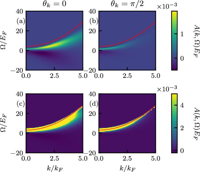
Figure 4. Single-particle spectral function for p-waves in different momentum directions: (a) and (b) are for binding energy Eb = −2EF and (c) and (d) are for binding energy Eb = 2EF. The red line in (a) and (b) indicates the free-atom contribution. The red line in (c) and (d) indicates the location of Ω = ξk. The results are calculated at a temperature T = 2EF. The effective range is kFRp = 1/30. In order to see the peak clearly, we set the color bar limit to 5 × 10⁻³ in (c) and (d). |
The single-particle spectral function of our system contains two main features: (i) the single-particle excitation peak A0 centered at the free-atom excitation energy Ω = ξk whose lifetime is determined by $\mathrm{Im}{\rm{\Sigma }}({\boldsymbol{k}},{\rm{\Omega }}={\xi }_{{\boldsymbol{k}}})$ and (ii) a threshold behavior from breaking a dimer, denoted by Aint.
On the BEC side, A0 is a delta peak with infinite lifetime
$\begin{eqnarray}{A}_{0}({\boldsymbol{k}},{\rm{\Omega }})=2\pi \delta ({\rm{\Omega }}-{\xi }_{{\boldsymbol{k}}}),\end{eqnarray}$
indicated by red lines in figures 4(a), (b) and 5(a), (b). This delta peak results from the fact that the denominator of Σ(k, Ω = ξk), ${\xi }_{{\boldsymbol{k}}}+{\xi }_{-{\boldsymbol{k}}+{\boldsymbol{q}}}-{\xi }_{{\boldsymbol{q}},b}-{E}_{b}={\left({\boldsymbol{k}}-{\boldsymbol{q}}/2\right)}^{2}-{E}_{b}$, is always positive when Eb < 0, which implies $\mathrm{Im}{\rm{\Sigma }}({\boldsymbol{k}},{\rm{\Omega }}={\xi }_{{\boldsymbol{k}}})=0$. Since the energy of an atom in the dimer is very different from the energy of a free atom, the spectral peaks of the free atom and that of an atom in a dimer are well separated. This result suggests that there is no coupling between the dimer state with negative binding energy and the scattering continuum with positive energy at this level of approximation.On the BCS side, there is only a quasi-bound state with positive binding energy, which has finite coupling with the scattering continuum. As a result, the peak from the single-particle excitation now gets a finite lifetime and merges into the dimer excitation, as shown in figures 4(c), (d) and 5(c), (d).
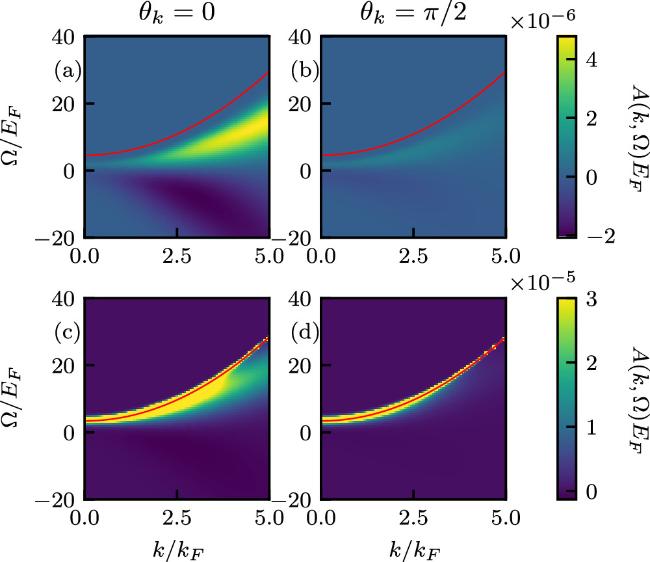
Figure 5. Single-particle spectral function for d-wave in different momentum directions: (a) and (b) are for binding energy Eb = −2EF and (c) and (d) are for binding energy Eb = 2EF. The red line in (a) and (b) indicates the free-atom contribution. The red line in (c) and (d) indicates the location of Ω = ξk. The results are calculated at temperature T = 2EF. The effective range is ${k}_{F}{v}_{d}^{1/3}=1/30$. In order to see the peak clearly, we set the color bar limit to 3 × 10⁻⁵ in (c) and (d). |
5. Momentum distribution
In this section, we calculate the momentum distribution of atoms, which can be expressed through the single-particle spectral function obtained in section 4 24 ) and (25 ). The above results verify the well-known k−2 and k0 tails as well as their relation with contacts for p- and d-wave interaction proposed in [18, 28].
$\begin{eqnarray}N({\boldsymbol{k}})={\int }_{-\infty }^{+\infty }\displaystyle \frac{{\rm{d}}{\rm{\Omega }}}{2\pi }{N}_{{\rm{B}}}({\rm{\Omega }})A({\boldsymbol{k}},{\rm{\Omega }}).\end{eqnarray}$
In the limit k = ∣k∣ → ∞ , we obtain the following asymptotic behavior for the momentum distribution: $\begin{eqnarray}{N}^{p}({\boldsymbol{k}})\approx \displaystyle \frac{16{\pi }^{2}}{{k}^{2}}{{ \mathcal C }}^{p}{\left|{Y}_{\mathrm{1,0}}({\theta }_{k})\right|}^{2},\end{eqnarray}$
$\begin{eqnarray}{N}^{d}({\boldsymbol{k}})\approx 16{\pi }^{2}{{ \mathcal C }}^{d}{\left|{Y}_{\mathrm{2,0}}({\theta }_{k})\right|}^{2},\end{eqnarray}$
where ${{ \mathcal C }}^{p}$ and ${{ \mathcal C }}^{d}$ are given by equations (The anisotropic nature of our system also manifests itself in the momentum distribution. Here we project the momentum distributions to the Legendre function Pℓ 32 ) and (33 ) is indicated by the gray dashed lines, which agree well with the numerical results from equation (31 ).
$\begin{eqnarray}{N}_{{\ell }}(k)={\int }_{0}^{\pi }{\rm{d}}{\theta }_{k}\cdot \sin {\theta }_{k}N({\boldsymbol{k}}){P}_{{\ell }}(\cos {\theta }_{k}).\end{eqnarray}$
The odd-ℓ components are always zero, which results from the spatial inversion symmetry. The even components are shown in figure 6. The analytic momentum tail in equations (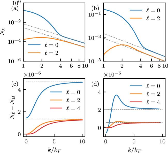
Figure 6. The momentum distribution projection to Legendre functions: (a) and (b) for p-waves and (c) and (d) for d-waves. The analytic tail in equations ( |
6. RF spectroscopy
Experimentally, the RF spectra are measured by coupling the hyperfine state σ2 to another hyperfine state labeled as σ3 by a RF pulse. This coupling can be described by the following Hamiltonian:
$\begin{eqnarray}{\hat{H}}_{L}=\displaystyle \sum _{{\boldsymbol{k}}}\left[{\hat{a}}_{{\boldsymbol{k}},{\sigma }_{2}}^{\dagger }{\hat{a}}_{{\boldsymbol{k}},{\sigma }_{3}}{e}^{{\rm{i}}\omega ^{\prime} t}+{\rm{h}}.{\rm{c}}.\right],\end{eqnarray}$
where $\omega ^{\prime} ={\nu }_{\mathrm{rf}}+\mu -{\mu }_{3}$, with νrf being the RF detuning. Then the RF spectrum, which describes the atom transfer rate from state σ2 to state σ3, can be expressed as a function of the single-particle spectral function [22] $\begin{eqnarray}I({\nu }_{\mathrm{rf}})=\displaystyle \frac{1}{2}\displaystyle \frac{1}{V}\displaystyle \sum _{{\boldsymbol{k}}}A({\boldsymbol{k}},{\xi }_{{\boldsymbol{k}}}-{\nu }_{\mathrm{rf}})\left[{N}_{{\rm{B}}}({\xi }_{{\boldsymbol{k}}}-{\nu }_{\mathrm{rf}})-{N}_{{\rm{B}}}({\xi }_{{\boldsymbol{k}},3})\right],\end{eqnarray}$
where ξk,3 = k2/2 − μ3. In numerical calculations we take the zero-density or vacuum limit where μ3 < 0 and ∣μ3∣ ≫ T, such that the σ3 state is nearly empty, i.e. NB(ξk,3) = 0. Now the RF spectrum can be simplified as $\begin{eqnarray}I({\nu }_{\mathrm{rf}})=\displaystyle \frac{1}{2}\displaystyle \frac{1}{V}\displaystyle \sum _{\vec{k}}A({\boldsymbol{k}},{\xi }_{{\boldsymbol{k}}}-{\nu }_{\mathrm{rf}}){N}_{{\rm{B}}}({\xi }_{{\boldsymbol{k}}}-{\nu }_{\mathrm{rf}}).\end{eqnarray}$
Following the analysis in section 4 , the RF spectra in our system also contain two features: (i) a single-particle peak I0(νrf) inherited from A0, corresponding to transferring a free atom from σ2 to σ3, and (ii) the part Iint(νrf) corresponding to transferring an atom in a bound or quasi-bound state from σ2 to σ3.
On the BEC side, as shown in figure 7(a), I0(νrf) is a delta peak located at νrf = 0
$\begin{eqnarray}{I}_{0}({\nu }_{\mathrm{rf}})=\pi \delta ({\nu }_{\mathrm{rf}})\displaystyle \frac{1}{V}\displaystyle \sum _{{\boldsymbol{k}}}{N}_{{\rm{B}}}({\xi }_{{\boldsymbol{k}}}),\end{eqnarray}$
which is well separated from Iint(νrf). Iint(νrf) has a threshold at νrf = −Eb, since the RF pulse must have enough energy to break the bound state in order to transfer an atom from state σ2 to state σ3.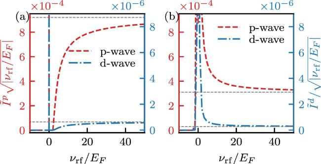
Figure 7. Dimensionless RF spectra of p- and d-waves at temperature T = 2EF: (a) for binding energy Eb = − 2EF and (b) for binding energy Eb = 2EF. The effective range ${k}_{F}{R}_{p}={k}_{F}{v}_{d}^{1/3}=1/30$. The gray dashed lines show the tail in equations ( |
On the BCS side, the weakly bound pair has a positive binding energy. Therefore a red detuned RF pulse is enough to transfer the atoms in the weakly bound pairs to state σ3. The free-atom delta peak is expanded and merged into the weakly bound pairs, as shown in figure 7(b)
In the large-frequency limit νrf → ∞ , we find the following asymptotic behavior from equation (37 ):24 ) and (25 ), which agrees well with the numerical calculation of equation (37 ).
$\begin{eqnarray}{I}^{p}({\nu }_{\mathrm{rf}})=\displaystyle \frac{1}{\sqrt{{\nu }_{\mathrm{rf}}}}{{ \mathcal C }}_{p},\end{eqnarray}$
$\begin{eqnarray}{I}^{d}({\nu }_{\mathrm{rf}})=\sqrt{{\nu }_{\mathrm{rf}}}{{ \mathcal C }}_{d}.\end{eqnarray}$
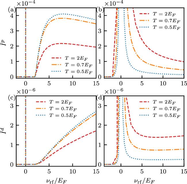
This also confirms the universal large-frequency tail proposed in [18, 28]. The gray dashed line in figure 7(b) indicates the contact density in equations (Next, we investigated the RF spectra at different temperatures, as shown in figure 8. On the BEC side, the RF spectrum is more significant at lower temperatures, provided the system is in the normal phase. When the temperature increases, the number of dimers becomes smaller. Therefore the atom number transfer to state σ3 from a dimer, i.e. the RF spectrum, becomes smaller. However, on the BCS side, because of a positive binding energy, the system tends to form more weakly bound dimers when the temperature increases. Therefore the temperature dependence of the RF spectrum on the BCS side shows the opposite behavior. It is worth noting that this reversed temperature dependence was also found in the temperature dependence of the contact density in figure 3.
Figure 8. Dimensionless RF $\tilde{I}$ spectrum at different temperatures: (a) and (b) are for p-waves and (c) and (d) for d-waves. Parts (a) and (c) are for binding energy Eb = −2EF, while parts (b) and (d) are for binding energy Eb = 2EF. The effective range is ${k}_{F}{R}_{p}={k}_{F}{v}_{d}^{1/3}=1/30$. |
Finally, we give an experimental estimation. In experiments, the number of atoms transferred to the hyperfine state σ3 in time t obeys the sum rule [4]
$\begin{eqnarray}\int \displaystyle \frac{{N}_{3}({\nu }_{\mathrm{rf}})}{t}{\rm{d}}{\nu }_{\mathrm{rf}}=\displaystyle \frac{{{\rm{\Omega }}}_{\mathrm{Rb}}^{2}}{2}\pi N,\end{eqnarray}$
where ΩRb is the Rabi frequency of the RF pulse. The sum rule of RF spectra in our work is $\begin{eqnarray}\int \tilde{I}({\tilde{\nu }}_{\mathrm{rf}}){\rm{d}}{\tilde{\nu }}_{\mathrm{rf}}=\displaystyle \frac{1}{2},\end{eqnarray}$
where ${\tilde{\nu }}_{\mathrm{rf}}={\hslash }{\nu }_{\mathrm{rf}}/{E}_{F}$, and $\begin{eqnarray}\tilde{I}=\displaystyle \frac{{E}_{F}}{{\hslash }}\displaystyle \frac{I({\nu }_{\mathrm{rf}})}{2\pi }\displaystyle \frac{V}{N},\end{eqnarray}$
is the dimensionless RF spectrum.By comparing equations (41 ) and (42 ), we can express the atom number transferred to the hyperfine states σ3 in time t as
$\begin{eqnarray}{N}_{3}=\displaystyle \frac{\hslash }{{E}_{F}}\tilde{I}t\cdot {{\rm{\Omega }}}_{\mathrm{Rb}}^{2}\pi N.\end{eqnarray}$
For a 105 41K atom cloud with density of 1013 cm−3, the estimated ${E}_{F}^{p}={2}^{-2/3}{E}_{F}^{d}\approx 5475h\mathrm{Hz}$, where h is the Planck constant. For a 0.16 ms RF pulse with Rabi frequency ΩRb = 30 × 2πkHz, the p-wave RF peak $\tilde{I}\approx 3\times {10}^{-4}$ results in N3 ≈ 1.6 × 10⁴, which is about 16% of all the atoms, transferred to the σ3 state. For the d-wave RF peak, we find $\tilde{I}\approx 3\times {10}^{-6}$ , and the number of atoms transferred is N3 ≈ 98, which is about 0.1% of total number of atoms. It seems that the p-wave RF spectrum might be reachable with the present experimental techniques while observation of the d-wave signal may be quite a challenge.7. Summary
In summary, we studied the p- and d-wave interacting Bose quantum gases in the normal phase using the Green’s function method in the spirit of the ladder diagram approximation. Firstly, we derived the contact density, which agrees well with the results of virial expansion. Then, we calculated the single-particle spectral function for different directions as well as the momentum distribution. The well-known large-k tails for p- and d-wave interaction were confirmed. Finally, we obtained the RF spectrum, investigated the temperature dependence of the RF spectrum and discovered a reversed temperature dependence on the BCS and BEC side of the FR. We also estimated the rate of transfer of atom number under a typical experimental setup. The results for p-waves might be reachable with the present method, while d-waves remain quite a challenge.