The aim of this work is to investigate anisotropic compact objects within the framework of f(G) modified theory of gravity. For our present work, we utilize Krori–Barua metrics, i.e., λ(r) = Xr2 + Y and β(r) = Zr2. We use some matching conditions of spherically symmetric spacetime with Bardeen's model as an exterior geometry. Further, we establish some expressions of energy density and pressure components to analyze the stellar configuration of Bardeen compact stars by assuming viable f(G) models. We examine the energy conditions for different stellar structures to verify the viability of our considered models. Moreover, we also investigate some other physical features, such as equilibrium condition, equation of state parameters, adiabatic index, stability analysis, mass function, surface redshift, and compactness factor, respectively. It is worthwhile to mention here for the current study that our stellar structure in the background of Bardeen's model is more viable and stable.
Adnan Malik, Ayesha Almas, Tayyaba Naz, Rubab Manzoor, M Z Bhatti. Detailed analysis of the relativistic configuration of Bardeen anisotropic spheres in modified f(G) gravity[J]. Communications in Theoretical Physics, 2024, 76(6): 065005. DOI: 10.1088/1572-9494/ad3f98
1. Introduction
In modern cosmology, the concept of the Universe's expansion stands as one of the cornerstone ideas, initially observed in the 1920s by astronomer Edwin Hubble, who noted that distant galaxies were receding from us at speeds proportional to their distances, prompting the development of the Big Bang theory, which suggests that the Universe originated from a singularity and has been expanding continuously since then. This expansion concept implies that the cosmos isn't static but is dynamically stretching out in all directions, carrying significant implications for our comprehension of the Universe, such as inferring that the Universe had a starting point, as proposed by the Big Bang theory. Initially hypothesized to decelerate due to gravitational pull, the Universe's expansion revealed an unexpected acceleration in 1998 through observations of extremely distant supernovae [1–5] by the Hubble Space Telescope, suggesting the presence of a mysterious force known as dark energy. Further evidence for this accelerating expansion comes from studies of the Cosmic Microwave Background [6–8] and investigations into the large-scale structure [9–12] of the Universe, sparking collaboration and inquiry among cosmologists and astrophysicists. The investigation regarding such cosmic expansion with the description of dark energy has been examined between the cosmologist and astrophysicists [13–16]. Efforts to understand this cosmic expansion and dark energy have taken various forms, including proposals for new constants related to dark energy and modifications to the Einstein–Hilbert action to formulate modified gravity theories to unravel the mysteries of the Universe's accelerating expansion and the enigmatic nature of dark energy.
Modified theories of gravity are crucial for discussing the behavior of stellar structures due to their potential to offer novel explanations for astrophysical phenomena that remain unexplained by conventional theories. Traditional gravity theories, such as general relativity, have been immensely successful in describing the behavior of gravity in many contexts. However, they encounter challenges when applied to extreme conditions, such as those found within compact stars or in the presence of dark matter and dark energy. Modified gravity theories provide an avenue for addressing these challenges by introducing additional degrees of freedom or modifying the gravitational equations themselves. By investigating stellar structures inside these altered frameworks, researchers may investigate the implications of various gravitational theories on star formation, structure, and development. This method not only improves our knowledge of gravity, but also offers insight on the underlying mechanisms that regulate celestial object behavior. Furthermore, researching stellar structures under modified gravity can provide new insights into processes like as gravitational collapse, neutron star mergers, and the behavior of matter in extreme gravitational fields, eventually improving our understanding of the Universe's complexities. Some of these are f(R) [17–20], f(G) [21–23], f(R, T) [24–27], f(Q) [28, 29], f(R, A) [30–32], f(R, φ) [33–35] and f(R, φ, X) [36–38] modified gravity theories. In these theories, the equations governing gravity are modified to include additional terms that could explain the observed acceleration of the Universe. Moreover, modified gravity theories have the potential to reconcile the observed cosmic acceleration with the prediction of general relativity, which is the most successful theory of gravity to date. Malik et al [39] explored some emerging properties of the stellar objects in the frame of the f(R, φ) gravity by employing the well-known Karmarkar condition. Recently, Naz et al [40] investigated the formation of compact stars using Tolman–Kuchowicz spacetime in f(G, T) theory of gravity. Ahmad et al [41] explored the charged stellar structures under embedded spacetime using the Karmarkar condition and spherically symmetric spacetime with the anisotropic source of fluid. Rashid et al [42] discussed the spherically symmetric solutions for describing the interior of a relativistic star in the context of f(R, T) modified theory of gravity by taking conformal killing vectors and Bardeen model. Malik along with his collaborators [43] investigated anisotropic stellar spheres in f(R, φ) gravity utilizing Tolman–Kuchowicz spacetime and derived the equations of motion for spherically symmetric spacetime. Mustafa et al [44] discussed the anisotropic nature of charged strange compact stars by considering the MIT bag model in the context of our universe's accelerated expansion scenario. The impacts of local density perturbations on the stability of self-gravitating compact objects by utilizing cracking technique within the context of f(R, T) gravity have been discussed in [45]. Recently, Malik et al employed the cracking technique in the Rastall gravity framework to assess how local density perturbations affect the stability of anisotropic stellar structures [75].
Indeed, the investigation of stellar structures within the framework of f(G) gravity is a highly appealing subject for researchers. The application of f(G) modified gravity to the study of stellar objects offers a unique opportunity to explore the effects of alternative theories of gravity on the behavior and properties of stars. By examining how modifications to gravity theories influence the structure, stability, and evolution of stars, researchers aim to deepen our understanding of both gravity itself and the astrophysical phenomena it governs. Through this exploration, new insights may emerge that could potentially revolutionize our comprehension of the Universe and its fundamental processes. Ilyas [46] investigated the stellar relativistic structure of anisotropic compact spheres in f(G) gravity under the presence of charge distribution by employing the Krori–Barua potential. Malik et al [47] explored the evaluation of anisotropic charge spheres in f(G) gravity by considering the Bardeen geometry. Shamir and Naz [48] explored some relativistic configurations of stellar objects for static spherically symmetric structures in the context of modified f(G) gravity, by exploiting the Tolman–Kuchowicz spacetime. The same authors [49] investigated some possible emergence of relativistic compact stellar objects in modified f(G) gravity using the Noether symmetry approach. They also [50] discussed the effect of charge configurations on relativistic compact stellar structures with isotropic matter distribution in the context of modified f(G) gravity. Ilyas [51] investigated some of the interior configurations of static anisotropic spherical stellar charged structures in the regime of f(G) gravity using the Krori and Barua metric. Malik et al [52] investigated the charged stellar structure in the background of the Gauss–Bonnet theory of gravity by utilizing the Tolman–Kuchowicz spacetime. Recently, Naz along with her collaborators [53] employed Karmarkar condition along with Finch–Skea ansatz to analyze the stellar configuration of compact stars.
Motivated by the literature and observations mentioned above, our study delves into the Bardeen anisotropic stellar sphere solution within the framework of f(G) modified gravity theory, employing the Krori–Barua metric. Our analysis demonstrates the smooth and continuous behavior of the metric tensor, validating the reliability of the obtained solutions. We explore the physical and stellar characteristics of the models obtained, deriving numerical values for relevant parameters. Furthermore, we extend our investigation to consider the proposed model's applicability to a variety of compact stars, expanding our understanding of its implications across different astrophysical contexts. The outline of current work is as follows: section 2 is based on developing the field equations of f(G) gravity for the anisotropic distribution of matter under the presence of charge. Section 3 deals with the matching conditions. Section 4 is composed of some physical features of compact stars. Concluding remarks are listed in last section.
2. Field equations of f(G) gravity
The action of modified f(G) theory of gravity is given as
where R&ugr;μηξ and R&ugr;μ represent the Riemannian and Ricci tensors respectively. Now, by varying equation (1) with respect to gηξ, we get the field equation for the f(G) gravity as
where, ρ, pr, pt represent the energy density, radial pressure and transverse pressure respectively. The four velocity vectors are defined as ${\zeta }_{\eta }={{\rm{e}}}^{\tfrac{a}{2}}{\delta }_{\eta }^{0}$ and ${\vartheta }_{\xi }={{\rm{e}}}^{\tfrac{b}{2}}{\delta }_{\xi }^{1}$. Further, the electromagnetic field Eηξ is given as
where λ and β are functions of radial coordinate r. Substituting all the values in equation (3), we get the expressions of energy density, radial pressure and tangential pressure as
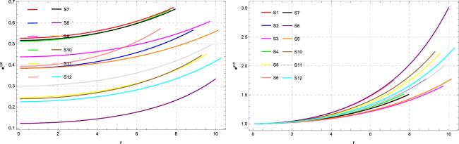
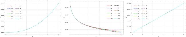
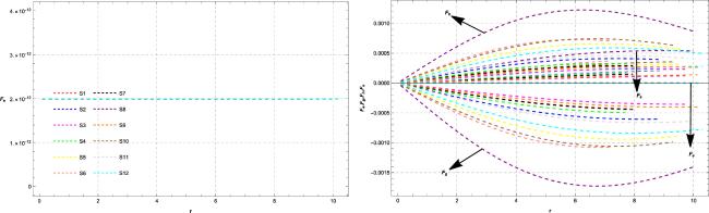
Here, prime ‘′' denotes the derivative with respect to radial coordinate r. For our present study, we assume the Krori–Barua potentials such as λ(r) = Xr2 + Y and β(r) = Zr2, where X, Y, and Z are unknown parameters [51]. However, we intend to determine these parameters later through a comparison method. Additionally, the behavior of the metric potential plays a crucial role in understanding the structure of stars. It is essential for the metric potential at the core to meet certain criteria, such as eλ(r=0)>0 and eβ(r=0)=1, to ensure physically viable stellar compositions. The analysis presented in figure 1 demonstrates that these constraints are indeed satisfied, confirming the physically stable behavior of the examined study. Subsequently, we employ compatible models of f(G) gravity theory to explore the behavior of compact stellar structures.
Initially, our focus lies on analyzing the characteristics of charged stellar configurations within the context of a power-law model incorporating logarithmic corrections, as expressed by the following equation:
where ψ2, τ2 and n are any arbitrary constant whereas ϱ2 > 0.
3. Boundary conditions
In this section, we compare the spherically symmetric spacetime with the Bardeen model serving as the exterior spacetime, and we establish matching conditions to derive solutions. The Bardeen model, utilized to characterize the exterior spacetime, is expressed as:
where ‘M' represents the mass of stellar structure. The Bardeen black hole may be regarded as a magnetic solution to Einstein equations combined with nonlinear electrodynamics [54]. The spacetime (14) finally becomes
To explore the physical attributes, it is imperative to establish a connection between the interior and exterior geometries of stars. To achieve this, we enforce continuity conditions for the metric potentials at the boundary (i.e., r = R ), resulting in the derivation of matching equations as follows:
where, − and + indicate the interior and exterior solution respectively. Now, by utilizing the above boundary condition (17), we obtain the unknown constants as
The set of equations (18)-(20) is very important for discussing the behavior of charged stellar structures, by using the observational data of various star candidates. Moreover, the numerical values of the parameter X, Y and Z for different stellar structures are given below in table 1.
Table 1. Undefined parameters of the compact star candidates for ϱ1 = ϱ2 = 2 and n = 1.
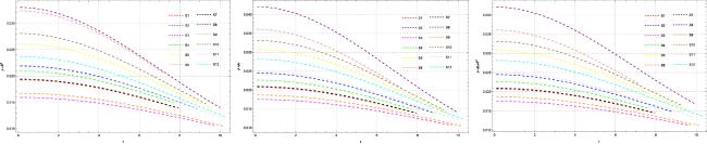
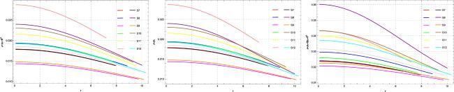
In this section, we delve into examining various physical features and stellar configurations of the model across different types of stars. It's widely acknowledged that for the model to align with astronomical observations, certain essential characteristics must be satisfied from both a theoretical and mathematical standpoint. These characteristics encompass a range of factors including energy density, pressure components, gradients, stability analysis, electric field intensity, equation of state (EoS) parameters, metric potentials, equilibrium conditions, energy conditions, anisotropy parameter, adiabatic index, and surface redshift.
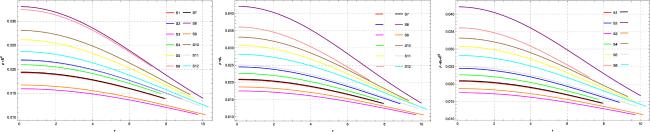
4.1. Energy density and pressure progression
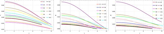
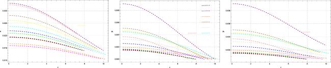
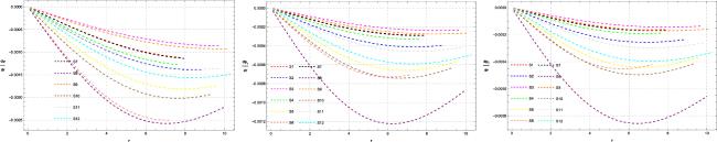
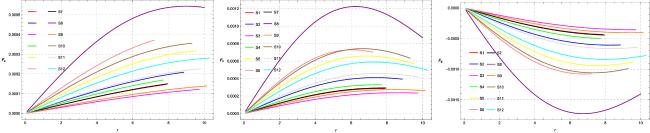
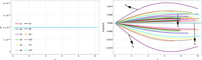
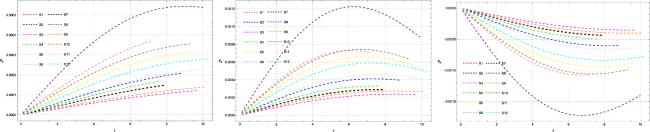
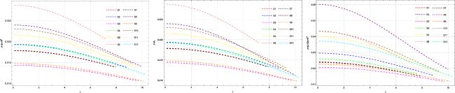
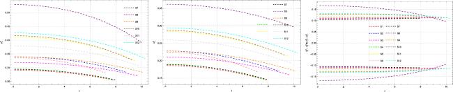
The graphical analysis of energy density (ρ), radial pressure (pr), and tangential pressure (pt) is non-negative, well-defined, and at its maximum at the core of the star. From figures 2 and 3, we observe that the graphical depiction of energy density and pressure components for the two presented models fulfills the criteria, being non-negative and maximum at the core before decreasing towards the boundary surface. Moreover, we provide a graphical representation of the gradients of density, radial pressure, and tangential pressure in figures 4 and 5, which are zero at the center and become negative when we move towards the boundary.
Figure 5. Evaluation of gradients of ρ, pr, and pt for Model II.
4.2. Anisotropy evolution
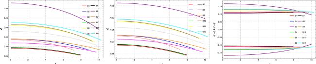
To investigate the stellar configuration of compact objects, we use the anisotropy parameter, which is a well-known feature in the stellar configuration. It can be determined by the formula [55] given as
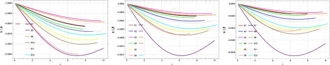
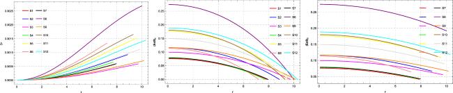
It is positive and directed outward if pt > pr; otherwise, it is negative and directed inward [56]. Through figures 6 and 7 (left plot), it is mentioned that the anisotropy parameter is positive and directed outward. In addition to this, it is zero at the core, which shows the stable nature of the star.
Figure 7. Evaluation of Δ, (EoS)r, and (EoS)t for model II.
4.3. Equation of state parameter
In literature, there are several equation of state parameters [57], but we prefer radial equation of state parameter (EoS)r and tangential equation of state parameter (EoS)t as
Moreover, the mandatory and adequate condition for these two parameters is that the range of (EoS)r and (EoS)t lies within the close intervals 0 and 1. It can be seen through figures 6 and 7 that the attributes of tangential and radial parameters of EoS are extreme at the core of the star, monotonically decreasing towards the boundary, and lie between 0 and 1.
4.4. Electric field intensity and charge density
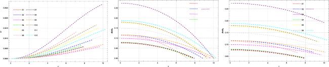
To discuss the anisotropic stellar configuration under the existence of charge, we analyze the nature of charge density as well as the electric field intensity. The fact that powerful electric fields are capable of bringing instabilities into the star's core is well established. If the charge density exceeds the 1020 coulombs then a quasi-static equilibrium state can be generated. This high level of charge density is associated with a very strong electric field that results in pairs being produced inside the star, which leads to instability. The evaluation of charge density graphically is maximal at the star's core and thereafter decreases as approaches the surface of the boundary of a star, as illustrated in figures 8 and 9 (middle plot). Further, the behavior of the electric field via graphical illustration shows an increasing nature and it is zero at the center of a stellar object. It is observed from the figures 8 and 9 (right plot), that the intensity of the electric field goes increasingly when we move toward the boundary surface and attain the highest value at the boundary point.
It can be observed from the figures 10–13 that all the forces show the balancing nature for both models, which means that our stars are in equilibrium condition.
For a physically stable nature, these conditions must be positive during the whole internal structure of the compact sphere. In the present study, it is observed through figures 14–17 that all of the above energy constraints for the considered star models are satisfied which shows the stable formation of two proposed models throughout the distribution.
where ${\nu }_{r}^{2}$ represents the radial velocity and ${\nu }_{t}^{2}$ denotes the transverse velocity. Additionally, we apply the Herrera cracking condition [60] to find the stability of a compact relativistic sphere. This condition states that the velocities must fall inside the interval [0, 1]. It is clearly obvious from figures 18 and 19 that both velocities met the Herrera requirement, which is $0\leqslant {\nu }_{r}^{2}\,{and}\,{\nu }_{t}^{2}\leqslant 1$. Furthermore, the criterion $-1\leqslant | {\nu }_{t}^{2}-{\nu }_{r}^{2}| \leqslant 0$ is proposed by Abreu et al [61] for the examination of stable or unstable stellar structure. Consequently, the ultimate goal of Abreu's condition is to show that unstable areas occur in stars if the tangential sound speed is greater than the radial sound speed. Therefore, it can be shown from the right plot of figures 18 and 19 that Abreu's limits have also been optimistic.
After Chandrasekhar [62] first demonstrated the concept of the radial adiabatic index for star stability, several cosmologists embraced it. The adiabatic index for stable spherically symmetric objects is larger than $\tfrac{4}{3}$, according to Hillebrandt and Steinmetz, [63]. When ${{\rm{\Gamma }}}_{r}=\tfrac{4}{3}$, a neutral equilibrium is established; when ${{\rm{\Gamma }}}_{r}\lt \tfrac{4}{3}$, an unstable stellar system is reached. Given the current environment, as seen in figure 20, we can observe that our proposed models are stable, as each star candidate has an adiabatic index greater than $\tfrac{4}{3}$.
Figure 20. Graphical variation of Γr for model I and II.
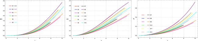
4.9. Mass, compactness factor and surface redshift
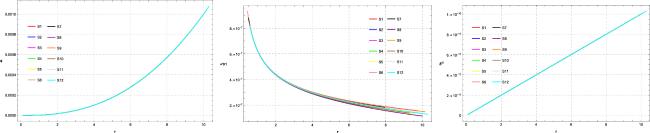
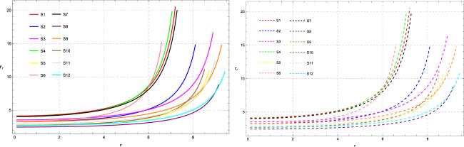
For the determination of hydrostatic static stability of relativistic compact spheres, the mass function [64] is useful. Here, for analyzing the stellar configuration of a charged compact sphere is given as
Moreover, the existence of our proposed model for the analysis of stellar configuration, its compactness factor, and surface redshift are important constraints. Whereas the compactness factor [65] for a compact star which is also known as the mass-radius ratio is expressed as
where u(r) represents the compactness factor. Furthermore, the existing limit value for the mass and radius ratio causes a limit value for more physical quality of factual concern. The surface Redshift [66] is described as
where Zs represents the surface Redshift function. According to Ivanov [66], for an anisotropic sphere without a cosmological constant model the value of surface Redshit is ≤5.211. From figures 21 and 22, it is observed that the graphical variation of mass function and compactness factor is positive, zero at the core, and increasing as approaches the surface of the boundary whereas the attribute of surface redshift function is positive and decreasing towards the boundary as well as it is ≤5.211. All these functions are positive. This shows that our model under consideration is stable.
Figure 22. Graphical evaluation of m(r), u(r), and Zs for model II.
In order to examine the inner structure of anisotropic compact spheres in the context of modified gravity theories, has attained great concentration among cosmologists throughout the decades. In light of this, the presented work aim is to investigate the analysis of anisotropic charged celestial bodies in the context of modified f(G) gravity. For this motivation, we utilize spherically symmetric spacetime along with the Krori–Barua metric potential. Furthermore, to find the unknown parameters, we considered the Bardeen geometry and compared it with the intrinsic metric. Moreover, to identify the stable configuration of our proposed model, we must ensure the validity of various physical features of the stellar structure for our model. Here, all of the essential results of physical features are summarized as:
•
Metric potentials are significant in predicting the nature of spacetime. From figure 1, it is noticed that the potentials are free from singularity and satisfying the necessary condition, i.e., eλ(r=0)>0 and eβ(r=0)=1.
•
Throughout the inner structure of the considered stars, the graphical variation of ρ, and both pressure components, i.e., pt and pr, shows non-negative, finite, and decreasing behavior as seen in figures 2 and 3. Further, the gradient graphs of density and pressure components must be non-positive which is illustrated in figures 4 and 5.
•
Figures 6 and 7 demonstrate the evolution of anisotropy, which is zero at the center as well as greater than zero whereas the equation of state parameter, i.e., ((EoS)r and (EoS)t), lies within the interval 0 and 1.
•
Electric field intensity is zero at the core and increasing in behavior whereas the graphical representation of charge density is decreasing in nature as shown in figures 8 and 9.
•
Figures 10 and 13 signifies the satisfying behavior of all forces and it also shows that all the forces compensate for each other effects.
•
Figures 14–17, show the stable configuration for the considered stars.
•
Figures 18 and 19 demonstrate that the sound speeds and Aberu condition is also satisfied.
•
Adiabatic index for all of the considered star models is satisfied as illustrated in figure 20.
•
Figures 21 and 22 implying the graphical variation of mass, compactness, and surface redshirt, which is positive and increasing with an increase of radii.
Hence, it is concluded that our present study satisfied all of the above-mentioned physical features as well as exhibited a stable nature of two proposed models for anisotropic charged distribution and our results agree with [67].
Conflict of interest
We, the authors, hereby declare that there are no competing interests of financial or personal nature.
Adnan Malik acknowledges the Grant No. YS304023912 to support his Postdoctoral Fellowship at Zhejiang Normal University, China.
RiessA G2004 Type Ia supernova discoveries at z > 1 from the Hubble Space Telescope: evidence for past deceleration and constraints on dark energy evolution Astrophys. J.607 665
ColeS2005 The 2dF Galaxy Redshift Survey: power-spectrum analysis of the final data set and cosmological implications Mon. Not. R. Astron. Soc.362 505 534
WangD2023 Observational constraints on a logarithmic scalar field dark energy model and black hole mass evolution in the Universe Eur. Phys. J. C83 1 14
MakM K, HarkoT2003 Anisotropic stars in general relativity Proceedings of the Royal Society of London. Series A: Mathematical, Physical and Engineering Sciences 459 393 408
GangopadhyayT2013 Strange star equation of state fits the refined mass measurement of 12 pulsars and predicts their radii Mon. Not. R. Astron. Soc.431 3216 3221


