


1. Introduction
Bootstrap, a novel yet promising method which has recently been studied in quantum mechanics, is a way to utilize the very general self-consistency condition and solve the system numerically. Developed in the 1960s and 70s [1], the method was later applied in large N systems [2–4], lattice theory [5–8], conformal field theory [9–13], as well as matrix models [14, 15]. This technique is also used to bootstrap the Dirac ensembles [16], some have integrated this method with artificial intelligence [17, 18]. And the bootstrap approaches used to find the eigen energies for bound states in recent papers are mostly inspired by Han [19]. Some papers have studied different systems using this method [20–25], and many have reported the accuracy and high precision of the method. In certain cases the bootstrap evolves into Dirac's ladder operator approach and can be solved analytically, suggesting some underlying mechanism of this method [26]. In this paper, we report an approach that can be seen as a classical correspondence to Han's.
Although widely studied in quantum mechanics, one can also apply the method to microcanonical ensembles as the fundamental relations of bootstrapping are still applicable and have their classical correspondence (3 ), (4 ), and (5 ) as ℏ → 0.
Nakayama [27] first introduced this method into the classical scenario, despite reporting the feasibility of the approach, he mentioned a peninsula in E < 0 which does not converge even for larger bootstrap matrices in the double-well potential. In this paper, we use a different approach that incorporates more information in phase space and thus exhibiting a much stronger constraint. We will see that the result of the double-well bootstrap in phase space cancels the sector region in E < 0 compared to the x only bootstrap. Also, it is worth mentioning that the similar approach is applied to the quantum anharmonic oscillator [28], which can be seen as the quantum version of our method.
We also investigate coulomb potential, a harmonic oscillator and a non-relativistic Toda model. The first two can be solved analytically (here by analytically, we mean that the averages of the observables can be written in a form of E) via the bootstrap approach which, however, are trivial cases. As for the non-relativistic Toda model, our approach in phase space once again demonstrates a more powerful restriction, maybe so overly powerful that we can merely see a few points in the result if the sample is not large enough. Since Hu [29] has discussed many models and derived lots of bootstrap equations, most of our models are modified versions of his.
Although our approach may have a stronger constraint, it still cannot converge to the exact solution in some places, like the non-relativistic Toda model. Not to mention that our approach consumes much more computing power, as the size of our bootstrap matrix is O(n4). However, the benefit is that we can easily achieve high precision when the result converges.
2. Microcanonical ensemble bootstrap
2.1. Bootstrap equations and matrices
Starting with the Hamiltonian we have5 ) with matrix and vectors7 ) should hold true for any vector α, the bootstrap matrix ${ \mathcal M }$ must embody the positive semi definiteness i.e. ${ \mathcal M }\succcurlyeq 0$, which is essentially an eigenvalue problem
$\begin{eqnarray}H=\displaystyle \frac{{p}^{2}}{2M}+V(x),\end{eqnarray}$
for a microcanonical ensemble, the average of an observable ${ \mathcal O }(x,p)$ is $\begin{eqnarray}\left\langle { \mathcal O }(x,p)\right\rangle =\displaystyle \frac{\int {\rm{d}}x{\rm{d}}p{ \mathcal O }(x,p)\delta (E-H)}{\int {\rm{d}}x{\rm{d}}p\delta (E-H)},\end{eqnarray}$
and we can easily find that $\begin{eqnarray}\left\langle \{H,{ \mathcal O }\}\right\rangle =0,\end{eqnarray}$
$\begin{eqnarray}\left\langle H{ \mathcal O }\right\rangle =E\left\langle { \mathcal O }\right\rangle ,\end{eqnarray}$
here $\{H,{ \mathcal O }\}$ is the poisson bracket. As for the positivity constraints, obviously for any observable ${ \mathcal O }$ we would have $\begin{eqnarray}\left\langle {{ \mathcal O }}^{* }{ \mathcal O }\right\rangle \geqslant 0,\end{eqnarray}$
and by writing the observable as a polynomial of certain observable o, ${ \mathcal O }={\sum }_{i=0}^{k}{a}_{i}{o}^{i}$, one can construct a bootstrap matrix which can be defined as $\begin{eqnarray}{{ \mathcal M }}_{{ij}}=\left\langle {\left({o}^{* }\right)}^{i}{o}^{j}\right\rangle ,\ \ i,j=0,1,...,k-1,\end{eqnarray}$
we can then rewrite the constraints ( $\begin{eqnarray}{{\boldsymbol{\alpha }}}^{\dagger }{ \mathcal M }{\boldsymbol{\alpha }}\geqslant 0,\end{eqnarray}$
as ( $\begin{eqnarray}\forall {\left({ \mathcal M }\right)}_{\mathrm{eigenvalue}}\geqslant 0.\end{eqnarray}$
When the observable ${ \mathcal O }$ is a coupling of two observables, say, A and B $\begin{eqnarray}{ \mathcal O }=\displaystyle \sum _{i,j=0}^{k-1}{a}_{i}{b}_{j}{A}^{i}{B}^{j},\end{eqnarray}$
$\begin{eqnarray}{{ \mathcal O }}^{* }{ \mathcal O }=\displaystyle \sum _{{i}_{1},{j}_{1},{i}_{2},{j}_{2}=0}^{k-1}{a}_{{i}_{1}}^{* }{b}_{{j}_{1}}^{* }{\left({B}^{* }\right)}^{{j}_{1}}{\left({A}^{* }\right)}^{{i}_{1}}{A}^{{i}_{2}}{B}^{{j}_{2}}{a}_{{i}_{2}}{b}_{{j}_{2}},\end{eqnarray}$
we can define two auxiliary matrices ${{ \mathcal M }}_{{ij}}^{0}={\left({B}^{* }\right)}^{j}{\left({A}^{* }\right)}^{i}$ and ${{ \mathcal M }}_{{ij}}^{1}={A}^{i}{B}^{j}$, the constraints can be written as $\begin{eqnarray}{{ \mathcal M }}_{{ij}}=\left\langle {\left({{ \mathcal M }}^{0}\otimes {{ \mathcal M }}^{1}\right)}_{{ij}}\right\rangle ,\ i,j=0,1,2,...,{k}^{2}-1,\end{eqnarray}$
$\begin{eqnarray}{ \mathcal M }\succcurlyeq 0.\end{eqnarray}$
2.2. Recursion formula
Taking ${ \mathcal O }$ as xmpn and substituting Hamiltonian (1 ) into (3 ) and (4 ), we immediately obtain
$\begin{eqnarray}\begin{array}{l}n\left\langle \displaystyle \frac{{\rm{d}}V}{{\rm{d}}x}{x}^{m}{p}^{n-1}\right\rangle =2{Em}\left\langle {x}^{m-1}{p}^{n-1}\right\rangle \\ \quad -2m\left\langle {{Vx}}^{m-1}{p}^{n-1}\right\rangle ,\\ \quad E\left\langle {x}^{m}{p}^{n}\right\rangle =\displaystyle \frac{1}{2m}\left\langle {x}^{m}{p}^{n+2}\right\rangle +\left\langle {{Vx}}^{m}{p}^{n}\right\rangle ,\end{array}\end{eqnarray}$
this would do the trick for the potential with polynomial of x. When the potential is in the form of exponentials, we need to take ${ \mathcal O }$ as emxpn $\begin{eqnarray}\begin{array}{l}n\left\langle \displaystyle \frac{{\rm{d}}V}{{\rm{d}}x}{{\rm{e}}}^{{mx}}{p}^{n-1}\right\rangle =2{Em}\left\langle {{\rm{e}}}^{{mx}}{p}^{n-1}\right\rangle -2m\left\langle V{{\rm{e}}}^{{mx}}{p}^{n-1}\right\rangle ,\\ E\left\langle {{\rm{e}}}^{{mx}}{p}^{n}\right\rangle =\displaystyle \frac{1}{2M}\left\langle {{\rm{e}}}^{{mx}}{p}^{n+2}\right\rangle +\left\langle V{{\rm{e}}}^{{mx}}{p}^{n}\right\rangle .\end{array}\end{eqnarray}$
2.3. Methodology framework
With the recursion formula (13 ) or (14 ) and a few initial values we can construct a whole bootstrap matrix ${ \mathcal M }$, and by testing the positive semi definiteness of the matrix the validity of the initial values can be determined. By doing so over all the possible initial values we will eventually find the allowed regions restricted by positivity constraint.
3. Numerical examples
3.1. Double-well potential
The Hamiltonian of a double-well potential can be written as13 ) we have16 ), (17 ), (18 ) and (19 ), plus the initial parameters E and $\left\langle {x}^{2}\right\rangle $, we can construct the bootstrap matrix ${ \mathcal M }$. The result is shown in figure 1. We also reproduced the result in [27] to make a comparison, which is shown in figure 2.
$\begin{eqnarray}H={p}^{2}-{x}^{2}+{x}^{4},\end{eqnarray}$
taking $M=\tfrac{1}{2}$ and with ( $\begin{eqnarray}\begin{array}{l}2(2n+m)\left\langle {x}^{m+3}{p}^{n-1}\right\rangle =2(m+n)\\ \quad \times \left\langle {x}^{m+1}{p}^{n-1}\right\rangle +2{mE}\left\langle {x}^{m-1}{p}^{n-1}\right\rangle ,\end{array}\end{eqnarray}$
$\begin{eqnarray}\begin{array}{l}\left\langle {{Hx}}^{m}{p}^{n}\right\rangle =E\left\langle {x}^{m}{p}^{n}\right\rangle =\left\langle {x}^{m}{p}^{n+2}\right\rangle \\ \quad -\left\langle {x}^{m+2}{p}^{n}\right\rangle +\left\langle {x}^{m+4}{p}^{n}\right\rangle ,\end{array}\end{eqnarray}$
plus $\left\langle \{H,{x}^{m}\}\right\rangle =0$, we get $\begin{eqnarray}\left\langle {x}^{m-1}p\right\rangle =0,\end{eqnarray}$
and for simplicity, here we assume that the average of x to the odd powers is 0, $\begin{eqnarray}\left\langle {x}^{m}\right\rangle =0,\ \ \mathrm{for}\,\mathrm{all}\,\mathrm{odd}\ m\end{eqnarray}$
with (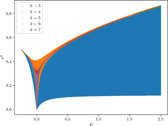
Figure 1. The allowed region in xp bootstrap. |
In contrast with [27], our result shows no peninsula when E is negative, as we include the information of the momentum. Although this xp bootstrap performs poorly when k = 3, the allowed region narrows down rapidly when k = 4 and it continues to shrink as k gets larger. Note that in our program the scale of the bootstrap matrix is k4, which is much larger compared to the single observable bootstrap program with the scale of k2. So in the case k = 5, the size of our bootstrap matrix is 625, about seven times bigger than that of the x bootstrap. However, the allowed region still does not shrink even when we set k = 25 for the x only bootstrap program, so we conclude that this bootstrap in phase space does have a much stronger constraint than the single observable one.
3.2. Harmonic oscillator and coulomb potential
Consider a harmonic oscillator, its Hamiltonian is18 ) also holds true, we only need the initial energy E to bootstrap. The result of the bootstrap is shown in figure 3, as we sample E from negative to positive, we can see that the negative energies are rejected by the bootstrap program.
$\begin{eqnarray}H={p}^{2}+{x}^{2},\end{eqnarray}$
and again, we can obtain the recursion formula $\begin{eqnarray}\begin{array}{l}2n\left\langle {x}^{m+1}{p}^{n-1}\right\rangle =2{Em}\left\langle {x}^{m-1}{p}^{n-1}\right\rangle \\ \quad -2m\left\langle {x}^{m+1}{p}^{n-1}\right\rangle ,\\ E\left\langle {x}^{m}{p}^{n}\right\rangle =\left\langle {x}^{m}{p}^{n+2}\right\rangle +\left\langle {x}^{m+2}{p}^{n}\right\rangle ,\end{array}\end{eqnarray}$
since $\left\langle {x}^{0}{p}^{0}\right\rangle =1$ and $\left\langle x\right\rangle =0$, and (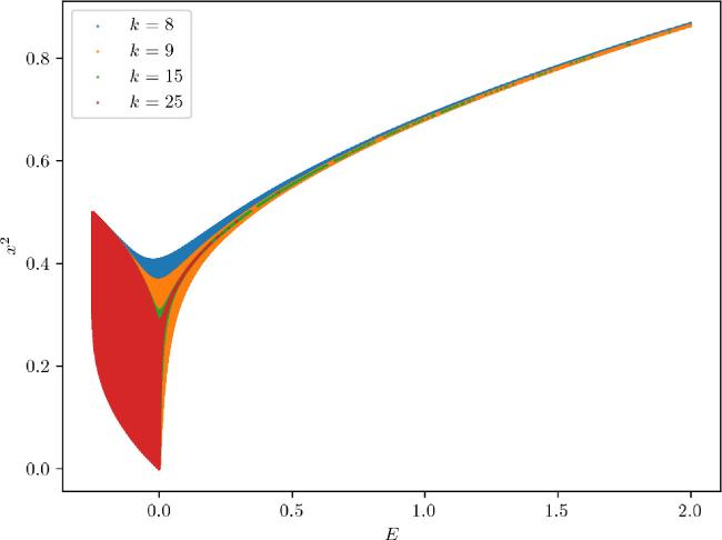
Figure 2. The allowed region in x bootstrap. |
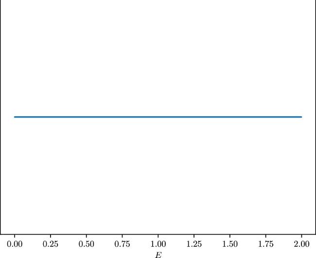
Figure 3. The allowed regions in xp bootstrap (k = 4) for harmonic oscillator. |
As for the coulomb potential, assume the Hamiltonian23 ) turn to 0, thus breaking the recursion. The initial value $\left\langle {r}^{-2}\right\rangle $ gives the exact information we need to patch up these points, together with equation (18 ), the result of bootstrap is shown in figure 5. We can see that our xp bootstrap excludes the positive E which will cause the r to go negative, but the nuisance here is that we need to pay extra attention to the numerical precision, for more details see the appendix .
$\begin{eqnarray}H={p}^{2}-\displaystyle \frac{1}{r}+\displaystyle \frac{1}{{r}^{2}},\end{eqnarray}$
here $-\tfrac{1}{r}+\tfrac{1}{{r}^{2}}$ is the effective potential. The recursion equations are $\begin{eqnarray}\begin{array}{l}2{mE}\left\langle {r}^{m-1}{p}^{n-1}\right\rangle =2(m-n)\left\langle {r}^{m-3}{p}^{n-1}\right\rangle \\ \quad +(n-2m)\left\langle {r}^{m-2}{p}^{n-1}\right\rangle ,\\ \quad E\left\langle {r}^{m}{p}^{n}\right\rangle =\left\langle {r}^{m}{p}^{n+2}\right\rangle -\left\langle {r}^{m-1}{p}^{n}\right\rangle +\left\langle {r}^{m-2}{p}^{n}\right\rangle .\end{array}\end{eqnarray}$
Substituting m = n = 1 into the first equation we can get $\begin{eqnarray}2E=-\left\langle {r}^{-1}\right\rangle ,\end{eqnarray}$
which is the Virial theorem. This time we only need E in the x bootstrap and the result is shown in figure 4. But for the xp bootstrap we also need the $\left\langle {r}^{-2}\right\rangle $ because at some points the coefficients in (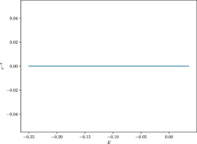
Figure 4. The allowed regions in x bootstrap (k = 8) for coulomb potential. |
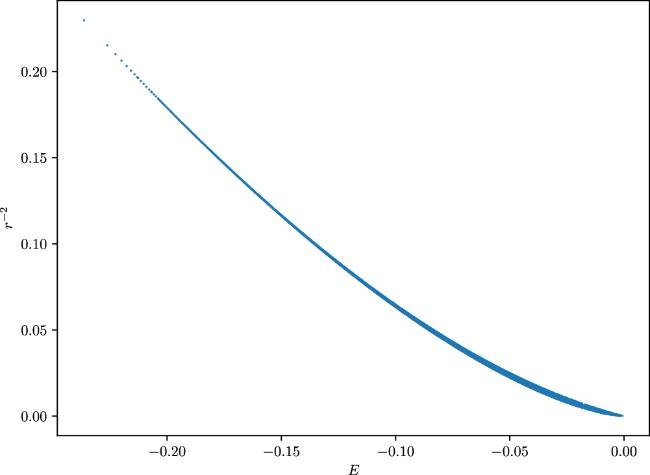
Figure 5. The allowed regions in xp bootstrap (k = 3) for coulomb potential. |
3.3. Non-relativistic Toda model
For a non-relativistic Toda model, the Hamiltonian could be written as
$\begin{eqnarray}H={p}^{2}+{{\rm{e}}}^{x}+{{\rm{e}}}^{-x},\end{eqnarray}$
the recursion equations are $\begin{eqnarray}\begin{array}{l}(n+2m)\left\langle {{\rm{e}}}^{m+1}{p}^{n-1}\right\rangle =2E\left\langle {{\rm{e}}}^{m}{p}^{n-1}\right\rangle \\ \quad +\,(n-2m)\left\langle {{\rm{e}}}^{m-1}{p}^{n-1}\right\rangle ,\\ E\left\langle {{\rm{e}}}^{{mx}}{p}^{n}\right\rangle =\left\langle {{\rm{e}}}^{{mx}}{p}^{n+2}\right\rangle \\ \quad +\,\left\langle {{\rm{e}}}^{(m+1)x}{p}^{n}\right\rangle +\left\langle {{\rm{e}}}^{(m-1)x}{p}^{n}\right\rangle ,\end{array}\end{eqnarray}$
and studying $\left\langle \{H,{{\rm{e}}}^{{mx}}\}\right\rangle $ we have $\begin{eqnarray}\left\langle {{\rm{e}}}^{\left(m-1)x\right.}p\right\rangle =0,\end{eqnarray}$
using the initial parameters E and $\left\langle {{\rm{e}}}^{x}\right\rangle $, the bootstrap result is shown in figure 6.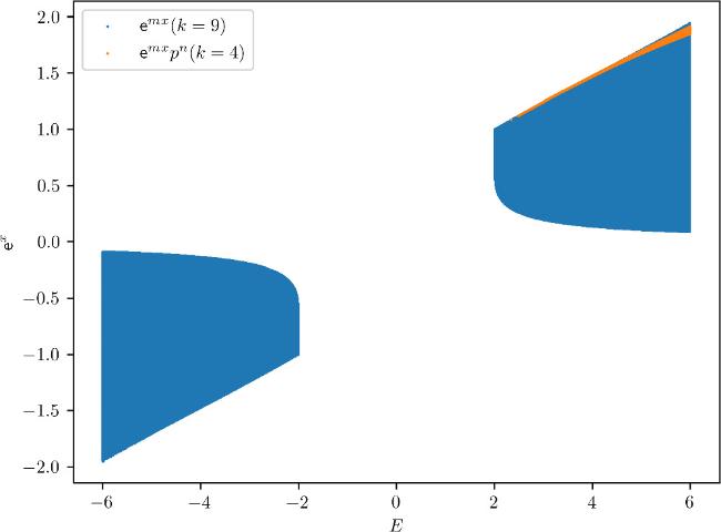
Figure 6. The allowed regions in xp bootstrap for non-relativistic Toda model. |
The two observables bootstrap shows a much stronger constraint than the single one, in this non-relativistic Toda mode the emx bootstrap even fails to reject the negative E, and results in a much larger region. Our approach may have better precision, yet the allowed region still tends to diverge when E goes large in figure 7.
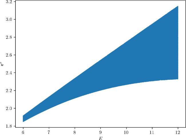
Figure 7. The allowed region diverges as E grows. |
4. Conclusions
In this paper, we study two different bootstrap approaches in various models, our approach outperforms the single observable bootstrap program in most cases. We have seen that it cancels the sector region in a double-well potential, excludes some invalid Es in both the harmonic oscillator and non-relativistic Toda model. Although it performs better and achieves a much higher precision, it still fails to converge to the exact solution, and even tends to diverge. Like in the situations that E → 0 in the double-well potential, E → ∞ in the non-relativistic Toda model, we might still be missing some information to pin point the final answer.
Appendix. Numerical details
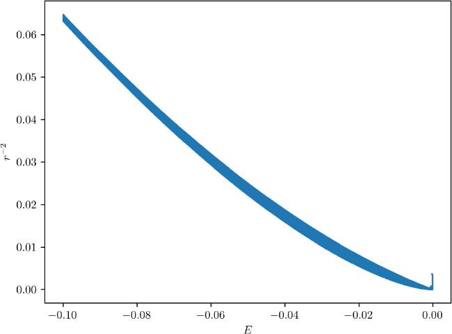
With the scale of the matrix growing at a fourth power rate, the floating-point precision becomes a bottleneck of our program as k grows. The typical double type in c++ no longer meets our need since the range of the eigenvalues can easily exceed 1018, thus leading to the loss of numerical precision in floating-point operations. In the coulomb potential above, this loss of precision will lead to some visible noise in the allowed region, resulting in a bulge where E is around 0 in figure A1. To eliminate this noise we set the precision in the code to 128 bits, as in figure 5.
Figure A1. The noise around E = 0 in coulomb potential. |