


1. Introduction
Quantum correlation in composite quantum systems is one of the main features of quantum mechanics and plays a crucial role in quantum information theory. Among various quantum correlations, entanglement [1, 2] is the most important. As an important quantum resource, entanglement has many practical applications, such as quantum dense coding [3], quantum teleportation [4] and quantum-measurement-based quantum computation [5]. The study of quantum nonlocality began with the pioneering work of Bell [6], showing that the strong correlations allowed by the quantum world cannot be explained by the familiar mechanism of space-time. Quantum nonlocality also has wide applications, such as quantum cryptography [7] and quantum communication [8]. The concept of Einstein–Podolsky–Rosen (EPR) steering was introduced by Schrödinger in 1935 as a response of the EPR paradox that was proposed in 1935 by Einstein, Podolsky and Rosen [9]. In 2007, the precise mathematical concept of EPR steering was proposed by Wiseman in [10]. In general, the three types of quantum correlations are inequivalent and there is a hierarchy between them: the Bell nonlocal state is necessarily EPR steerable, while the EPR steerable state is not necessarily Bell nonlocal; and the EPR steerable state is necessarily entangled, while the entangled state is not necessarily EPR steerable. In recent decades, many researchers have paid more attention to the detection and quantification of Bell nonlocality, entanglement and EPR steering [11–20].
A quantum network is the basis of long-distance and networked quantum communication and plays an important role in quantum communication, quantum computation and quantum measurement [21]. The wide applications of quantum networks are based on an experiment called entanglement swapping in [22–24], which shows that quantum systems that never interacted in the past can become entangled. With these generated correlations in quantum networks, many quantum communications tasks can be achieved [25, 26]. As a result of their significance, much research has been devoted to investigating quantum correlations generated by quantum networks, such as Bell nonlocality in networks [27], network entanglement [28], network steering [29] and network coherence [30], which are different from conventional quantum correlations. In contrast to the above works, which are focused on examining some specific quantum correlations pertaining to quantum networks, the authors in [31] recently studied the conventional quantum correlations of all post-measurement states in a generalized entanglement swapping protocol. In this protocol, they characterized the variations of quantum correlations of all post-measurement states with respect to the initial quantum states and quantum measurements with parameters. With this work, scholars can control the amount of quantum correlations in post-measurement states by adjusting the parameters, which is meaningful in practical applications.
In the present paper, we examine the conventional quantum correlations of all post-measurement states in a general chain-type quantum network protocol. In this protocol, each of two neighboring observers share any Bell state and all intermediate observers perform some positive-operator-valued measurements (POVMs) with some parameters. This paper is organized as follows. In section 2 , we recall the (generalized) entanglement swapping protocol, and the known quantifications of Bell nonlocality, EPR steering and entanglement. In section 3 , we consider all post-measurement states between any two observers in a chain network with any n parties when each of two neighboring parties share any Bell state and all intermediate parties perform some POVMs with parameter λ. We obtain the concrete forms of all post-measurement states and, particularly, a specific calculation process for the case n = 5 is given. Section 4 is devoted to discussing three different quantum correlations of all these post-measurement states. Moreover, we illustrate it for n = 5 by plotting the three quantum correlations of post-measurement states as the parameter λ varies. Some concluding remarks are given in section 5 . The proof of the main results is provided in the appendix .
2. Preliminaries
In this section, we recall the entanglement swapping protocol, the quantifications of Bell nonlocality, entanglement and EPR steering, and the generalized entanglement swapping protocol.
2.1. Entanglement swapping network
The entanglement swapping network (see figure 1) is a network of three parties consisting of Alice, Bob and Charlie, and two independent sources, S1 and S2, shared between Alice, Bob and Charlie. Every quantum state in this network has the form $\rho ={\rho }_{{{AB}}_{1}}\otimes {\rho }_{{B}_{2}C}$ with state space H = HA ⨂ HB ⨂ HC, where ${H}_{B}={H}_{{B}_{1}}\otimes {H}_{{B}_{2}}$. Assume that Alice and Bob share the quantum state ${\rho }_{{{AB}}_{1}}$ chosen from any one of four Bell states
$\begin{eqnarray}\{| {\psi }_{1}\rangle \langle {\psi }_{1}| ,| {\psi }_{2}\rangle \langle {\psi }_{2}| ,| {\psi }_{3}\rangle \langle {\psi }_{3}| ,| {\psi }_{4}\rangle \langle {\psi }_{4}| \},\end{eqnarray}$
where $| {\psi }_{1}\rangle =\tfrac{| 00\rangle +| 11\rangle }{\sqrt{2}},| {\psi }_{2}\rangle =\tfrac{| 00\rangle -| 11\rangle }{\sqrt{2}},| {\psi }_{3}\rangle =\tfrac{| 01\rangle +| 10\rangle }{\sqrt{2}},| {\psi }_{4}\rangle =\tfrac{| 01\rangle -| 10\rangle }{\sqrt{2}}$, meanwhile, Bob shares any one of four Bell states, written as ${\rho }_{{B}_{2}C}$, with Charlie. Due to the independence of sources S1 and S2, Alice and Charlie are not entangled with each other. Once Bob performs a Bell state measurement ${\{| {\psi }_{i}\rangle \langle {\psi }_{i}| \}}_{i=1}^{4}$, Alice and Charlie become entangled [22].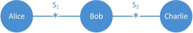
Figure 1. The entanglement swapping network consists of three parties, Alice, Bob and Charlie, and two sources, S1 shared by Alice and Bob, and S2 shared by Bob and Charlie. In this network, the two independent sources respectively produce the Bell state and Bob performs Bell state measurement. |
2.2. Bell nonlocality
In a typical Bell experiment, two spatially separated observers Alice and Bob receive particles from a common source S. After receiving their particles, each observer performs a measurement on it. Denote the inputs of Alice and Bob by x, y with the corresponding outputs a, b, respectively. The resultant correlation is said to be local if the joint probability distribution P(a, b∣x, y) can be decomposed into the following form:
$\begin{eqnarray*}P(a,b| x,y)={\int }_{\lambda }\rho (\lambda )p(a| x,\lambda )p(b| y,\lambda ){\rm{d}}\lambda ,\end{eqnarray*}$
where λ characterizes the hidden variable of S with probability distribution ρ(λ), and p(a∣x, λ) (p(b∣y, λ)) is the probability distribution of Alice's (Bob's) measurement outcome a (b), which depends on the measurement choice x (y) and hidden variable λ; otherwise, the correlation is said to be nonlocal [32].To detect Bell nonlocality, the most famous criterion is Clauser–Horne–Shimony–Holt (CHSH) inequality ([11]). Assume that both Alice and Bob have two binary measurement choices, denoted respectively by {A0, A1} and {B0, B1}. It is shown that all local correlations must satisfy the following inequality:
$\begin{eqnarray*}\begin{array}{l}{{ \mathcal B }}_{\mathrm{CHSH}}=\langle {A}_{0}{B}_{0}\rangle \\ \quad +\langle {A}_{0}{B}_{1}\rangle +\langle {A}_{1}{B}_{0}\rangle -\langle {A}_{1}{B}_{1}\rangle \leqslant 2.\end{array}\end{eqnarray*}$
Let HA, HB be finite dimensional complex Hilbert spaces. Denote by ${ \mathcal B }({H}_{A}\otimes {H}_{B})$ the algebra of all bounded linear operators in the composite space HA ⨂ HB and ${ \mathcal S }({H}_{A}\otimes {H}_{B})$ the state space on HA ⨂ HB. If $\dim {H}_{A}=\dim {H}_{B}=2$, then any 2-qubit state $\rho \in { \mathcal S }({H}_{A}\otimes {H}_{B})$ can be written as
$\begin{eqnarray*}\begin{array}{l}\rho =\displaystyle \frac{1}{4}({\mathbb{I}}\otimes {\mathbb{I}}+{\vec{r}}_{A}\cdot \vec{\sigma }\otimes {\mathbb{I}}\\ \quad +{\mathbb{I}}\otimes {\vec{r}}_{B}\cdot \vec{\sigma }+\displaystyle \sum _{i,j}{t}_{{ij}}{\sigma }_{i}\otimes {\sigma }_{j})\end{array}\end{eqnarray*}$
under the Pauli basis {σx, σy, σz}, where $\vec{\sigma }=({\sigma }_{x},{\sigma }_{y},{\sigma }_{z})$, ${\vec{r}}_{A}$ (${\vec{r}}_{B}$) represents the Bloch vector of Alice's (Bob's) reduced state, and ${\mathbb{I}}\in { \mathcal B }({H}_{A\setminus B})$ is the identity operator. Write Rρ = (tij). Then ${t}_{{ij}}=\mathrm{Tr}[\rho ({\sigma }_{i}\otimes {\sigma }_{j})]$ with i, j ∈ {x, y, z}. Here, Rρ is called the correlation matrix (CM) of ρ. In [33], the authors proved that the maximal value of CHSH inequality is $\begin{eqnarray*}{{ \mathcal B }}_{\mathrm{CHSH}}^{\max }=2\sqrt{{t}_{1}+{t}_{2}},\end{eqnarray*}$
where t1 and t2 are two greater eigenvalues of ${R}_{\rho }^{\dagger }{R}_{\rho }$. Thus, ρ violates the CHSH inequality, if and only if, $\sqrt{{M}_{\rho }}\gt 1$ with Mρ = t1 + t2. In [31], a measure of Bell nonlocality is given by $\begin{eqnarray}{ \mathcal N }(\rho )=\max \left\{0,\displaystyle \frac{\sqrt{{M}_{\rho }}-1}{\sqrt{2}-1}\right\}.\end{eqnarray}$
Obviously, ${ \mathcal N }(\rho )\gt 0$ implies that ρ violates the above CHSH inequality.2.3. EPR steering
EPR steering is a kind of quantum correlation lying in entanglement and Bell nonlocality [10]. Suppose that Alice and Bob share a quantum state ρ. If Alice performs a POVM Ma∣x labeled by x with outcome a, then the obtained unnormalized state of Bob is ${\sigma }_{a| x}={\mathrm{Tr}}_{{\rm{A}}}[({M}_{a| x}\otimes {\mathbb{I}})\rho ]$. We say that σa∣x has a local hidden state (LHS) form if it can be written as
$\begin{eqnarray*}{\sigma }_{a| x}=\displaystyle \sum _{\lambda }p(\lambda )p(a| x,\lambda ){\sigma }_{\lambda },\end{eqnarray*}$
where λ is a hidden variable with probability distribution p(λ), σλ is the hidden state of Bob and p(a∣x, λ) is a local response function of Alice. Furthermore, ρ is called EPR unsteerable from Alice to Bob if σa∣x always admits such an LHS decomposition under any POVMs. Thus, if some POVMs exist, such that σa∣x does not admit such an LHS decomposition, then ρ is EPR steerable from Alice to Bob.For the quantification of EPR steering, the authors in [34] proposed an EPR steering measure for any 2-qubit quantum state $\rho \in { \mathcal S }({H}_{A}\otimes {H}_{B})$:
$\begin{eqnarray}{ \mathcal S }(\rho )=\max \left\{0,\displaystyle \frac{\sqrt{{\wedge }_{\rho }}-1}{\sqrt{n}-1}\right\}\ \ \mathrm{with}\ \ {\wedge }_{\rho }={t}_{1}+{t}_{2}+{t}_{3},\end{eqnarray}$
where ti for i = 1, 2, 3 are the singular values of the CM Rρ. It is shown that ${ \mathcal S }(\rho )\gt 0$ implies that ρ is EPR steerable.2.4. Entanglement
Entanglement is also a type of important quantum correlation. Assume that $\rho \in { \mathcal S }({H}_{A}\otimes {H}_{B})$ is any quantum state. We say that ρ is separable if there are convex weights {pi} and quantum states $\{{\rho }_{i}^{A}\}\subset { \mathcal S }({H}_{A})$, $\{{\rho }_{i}^{B}\}\subset { \mathcal S }({H}_{B})$ such that $\rho ={\sum }_{i}{p}_{i}{\rho }_{i}^{A}\otimes {\rho }_{i}^{B};$ otherwise, ρ is entangled ([1, 2]).
For any 2-qubit quantum state ρ, an entanglement measure called negativity is proposed in [35]:
$\begin{eqnarray*}{ \mathcal E }(\rho )=\parallel {\rho }^{{T}_{B}}{\parallel }_{1}-1,\end{eqnarray*}$
where $\parallel {\rho }^{{T}_{B}}{\parallel }_{1}$ denotes the trace norm of the partial transpose of ρ with respect to subsystem B. Then it is clear that $\begin{eqnarray}{ \mathcal E }(\rho )=2\max \{0,-\mu \},\end{eqnarray}$
where μ is the minimum eigenvalue of ${\rho }^{{T}_{B}}$. It is shown that any 2-qubit quantum state ρ is entangled, if and only if, ${ \mathcal E }(\rho )\gt 0$.2.5. Generalized entanglement swapping
Concretely, suppose that Alice and Bob share any Bell state ∣ψj⟩⟨ψj∣, Bob and Charlie share any Bell state ∣ψl⟩⟨ψl∣, j, l ∈ {1, 2, 3, 4}, and Bob performs a POVM
$\begin{eqnarray*}\begin{array}{l}E=\{{E}_{1},{E}_{2},{E}_{3},{E}_{4}\}\ \ \mathrm{with}\ \ {E}_{i}=\lambda | {\psi }_{i}\rangle \langle {\psi }_{i}| \\ \quad +\displaystyle \frac{1-\lambda }{4}{\mathbb{I}},\ \lambda \in [0,1].\end{array}\end{eqnarray*}$
They respectively obtained the post-measurement states between Alice and Charlie, Alice and Bob, and Bob and Charlie. Whether these post-measurement states are nonlocal, entanglement or EPR steering with different values of λ was also discussed.3. Chain-type quantum network protocol
In this section, we consider the chain-type quantum network scenario (see figure 2). This network contains n (n ≥ 3) parties, denoted by A1,…, An, and n − 1 independent sources S1, …, Sn−1. Every quantum state in the network has the form
$\begin{eqnarray*}\rho ={\rho }_{\mathrm{1,2}}\otimes {\rho }_{\mathrm{2,3}}\otimes \cdots \otimes {\rho }_{n-1,n}\end{eqnarray*}$
with state space H = H1 ⨂ H2 ⨂ ⋯ ⨂ Hn, where Hk = Hk,1 ⨂ Hk,2 for k = 2,…,n − 1. Write H1 = H1,2 and Hn = Hn,1. So ${\rho }_{j,j+1}\in { \mathcal S }({H}_{j,2}\otimes {H}_{j+\mathrm{1,1}})$ (j ∈ {1,…,n − 1}), which is shared by Aj and Aj+1.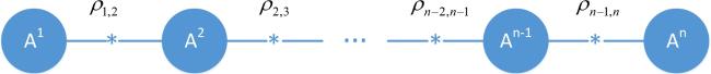
Figure 2. The chain network consists of n parties (n ≥ 3) A1, A2, …, An−1, An, where observers A1, A2 share quantum states ρ1,2, …, An−1, An shares quantum states ρn−1,n, and the observers A2, …, An−1 perform some POVMs. |
In the network of figure 2, suppose that ρj,j+1 (j ∈ {1,…,n − 1}) is chosen from one of the four Bell states in equation (1 ) and each observer Ak (k ∈ {2,…,n − 1}) performs a POVM ${E}^{k}=\{{E}_{1}^{k},{E}_{2}^{k},{E}_{3}^{k},{E}_{4}^{k}\}$ with
$\begin{eqnarray}{E}_{i}^{k}={\lambda }_{k}| {\psi }_{i}\rangle \langle {\psi }_{i}| +\displaystyle \frac{1-{\lambda }_{k}}{4}{\mathbb{I}},\ \ i\in \{1,2,3,4\},\end{eqnarray}$
where λk ∈ [0, 1] is the parameter of Ek. In the following, we will calculate the forms of all post-measurement states shared between Ap and Aq under this specific circumstance.Denote by ${\sigma }_{p,q}^{n}({u}_{1},\cdots ,{u}_{n-1};{v}_{2},\cdots ,{v}_{n-1})$ the post-measurement state shared between Ap and Aq with 1 ≤ p < q ≤ n, where uj, vk ∈ {1, 2, 3, 4}, j ∈ {1,…,n − 1}, k ∈ {2,…,n − 1}, uj represents the value of i in ρj,j+1 = ∣ψi⟩⟨ψi∣; and vk represents the value of i in the measurement operator Eki. For simplicity, write ${\sigma }_{p,q}^{n}(\vec{{\boldsymbol{u}}};\vec{{\boldsymbol{v}}})={\sigma }_{p,q}^{n}({u}_{1},\cdots ,{u}_{n-1};{v}_{2},\cdots ,{v}_{n-1})$ with $\vec{{\boldsymbol{u}}}=({u}_{1},\cdots ,{u}_{n-1})$ and $\vec{{\boldsymbol{v}}}=({v}_{2},\cdots ,{v}_{n-1})$. Let ${c}_{i}({\sigma }_{p,q}^{n}(\vec{{\boldsymbol{u}}};\vec{{\boldsymbol{v}}}))$ stand for the sum of the number of appearances of i in up, up+1, ⋯ ,uq−1 and vp+1, ⋯ ,vq−1, where p + 1 ≤ q − 1.
For example, consider n = 5, p = 2, q = 3, $\vec{{\boldsymbol{u}}}\,=(1,1,2,2)$ and $\vec{{\boldsymbol{v}}}=(2,3,3)$. In this case, from the above definition, we have ρ1,2 = ρ2,3 = ∣ψ1⟩⟨ψ1∣ and ρ3,4 =ρ4,5 = ∣ψ2⟩⟨ψ2∣; the measurement operators acting on observers A2, A3 and A4 are, respectively, ${E}_{2}^{2}\,={\lambda }_{2}| {\psi }_{2}\rangle \langle {\psi }_{2}| +\tfrac{1-{\lambda }_{2}}{4}{\mathbb{I}}$, ${E}_{3}^{3}={\lambda }_{3}| {\psi }_{3}\rangle \langle {\psi }_{3}| +\tfrac{1-{\lambda }_{3}}{4}{\mathbb{I}}$ and ${E}_{3}^{4}\,={\lambda }_{4}| {\psi }_{3}\rangle \langle {\psi }_{3}| +\tfrac{1-{\lambda }_{4}}{4}{\mathbb{I}};$ and ${c}_{1}({\sigma }_{2,3}^{5}(\vec{{\boldsymbol{u}}};\vec{{\boldsymbol{v}}}))=1$, ${c}_{2}({\sigma }_{2,3}^{5}(\vec{{\boldsymbol{u}}};\vec{{\boldsymbol{v}}}))\,=0$, ${c}_{3}({\sigma }_{2,3}^{5}(\vec{{\boldsymbol{u}}};\vec{{\boldsymbol{v}}}))=0$, ${c}_{4}({\sigma }_{2,3}^{5}(\vec{{\boldsymbol{u}}};\vec{{\boldsymbol{v}}}))=0.$
With these notations, we can obtain the concrete forms of any post-measurement states ${\sigma }_{p,q}^{n}(\vec{{\boldsymbol{u}}};\vec{{\boldsymbol{v}}})$:appendix .
$\begin{eqnarray}{\sigma }_{p,q}^{n}(\vec{{\boldsymbol{u}}};\vec{{\boldsymbol{v}}})={\alpha }_{p,q}| {\psi }_{i}\rangle \langle {\psi }_{i}| +\displaystyle \frac{1-{\alpha }_{p,q}}{4}{{\mathbb{I}}}_{4},\end{eqnarray}$
where αp,q = s(λp)λp+1 ⋯ λq−1s(λq) and $\begin{eqnarray}i=\left\{\begin{array}{l}1\ \ \mathrm{if}\ {c}_{3}({\sigma }_{p,q}^{n}(\vec{{\boldsymbol{u}}};\vec{{\boldsymbol{v}}}))+{c}_{4}({\sigma }_{p,q}^{n}(\vec{{\boldsymbol{u}}};\vec{{\boldsymbol{v}}}))\ \mathrm{is}\ \mathrm{even}\ \mathrm{and}\ {c}_{2}({\sigma }_{p,q}^{n}(\vec{{\boldsymbol{u}}};\vec{{\boldsymbol{v}}}))+{c}_{4}({\sigma }_{p,q}^{n}(\vec{{\boldsymbol{u}}};\vec{{\boldsymbol{v}}}))\ \mathrm{is}\ \mathrm{even},\\ 2\ \ \mathrm{if}\ {c}_{3}({\sigma }_{p,q}^{n}(\vec{{\boldsymbol{u}}};\vec{{\boldsymbol{v}}}))+{c}_{4}({\sigma }_{p,q}^{n}(\vec{{\boldsymbol{u}}};\vec{{\boldsymbol{v}}}))\ \mathrm{is}\ \mathrm{even}\ \mathrm{and}\ {c}_{2}({\sigma }_{p,q}^{n}(\vec{{\boldsymbol{u}}};\vec{{\boldsymbol{v}}}))+{c}_{4}({\sigma }_{p,q}^{n}(\vec{{\boldsymbol{u}}};\vec{{\boldsymbol{v}}}))\ \mathrm{is}\ \mathrm{odd},\\ 3\ \ \mathrm{if}\ {c}_{3}({\sigma }_{p,q}^{n}(\vec{{\boldsymbol{u}}};\vec{{\boldsymbol{v}}}))+{c}_{4}({\sigma }_{p,q}^{n}(\vec{{\boldsymbol{u}}};\vec{{\boldsymbol{v}}}))\ \mathrm{is}\ \mathrm{odd}\ \mathrm{and}\ {c}_{2}({\sigma }_{p,q}^{n}(\vec{{\boldsymbol{u}}};\vec{{\boldsymbol{v}}}))+{c}_{4}({\sigma }_{p,q}^{n}(\vec{{\boldsymbol{u}}};\vec{{\boldsymbol{v}}}))\ \mathrm{is}\ \mathrm{even},\\ 4\ \ \mathrm{if}\ {c}_{3}({\sigma }_{p,q}^{n}(\vec{{\boldsymbol{u}}};\vec{{\boldsymbol{v}}}))+{c}_{4}({\sigma }_{p,q}^{n}(\vec{{\boldsymbol{u}}};\vec{{\boldsymbol{v}}}))\ \mathrm{is}\ \mathrm{odd}\ \mathrm{and}\ {c}_{2}({\sigma }_{p,q}^{n}(\vec{{\boldsymbol{u}}};\vec{{\boldsymbol{v}}}))+{c}_{4}({\sigma }_{p,q}^{n}(\vec{{\boldsymbol{u}}};\vec{{\boldsymbol{v}}}))\ \mathrm{is}\ \mathrm{odd},\end{array}\right.\end{eqnarray}$
$s({\lambda }_{k})=\tfrac{1}{2}[1-{\lambda }_{k}+\sqrt{(1-{\lambda }_{k})(1+3{\lambda }_{k})}]$ if k ∈ {p + 1,…,q − 1}; s(λ1) = 1; and s(λn) = 1 with n ≥ 3. The detailed derivation is presented in the Particularly, if all parties A2, …, An−1 in the network of figure 2 perform the same measurement, i.e. λ2 = ⋯ = λn−1, then the post-measurement states in equation (6 ) reduce to7 ), $s(\lambda )=\tfrac{1}{2}[1-\lambda +\sqrt{(1-\lambda )(1+3\lambda )}];$ ξ = 0 if p = 1 and q = n; ξ = 1 if p = 1 or q = n; ξ = 2 if p ≠ 1 and q ≠ n.
$\begin{eqnarray}{\sigma }_{p,q}^{n}(\vec{{\boldsymbol{u}}};\vec{{\boldsymbol{v}}})=s{\left(\lambda \right)}^{\xi }{\lambda }^{q-p-1}| {\psi }_{i}\rangle \langle {\psi }_{i}| +\displaystyle \frac{1-s{\left(\lambda \right)}^{\xi }{\lambda }^{q-p-1}}{4}{{\mathbb{I}}}_{4},\end{eqnarray}$
where the value of i is the same as that of equation (In fact, take ρ1,2 = ρ2,3 = ∣ψ1⟩⟨ψ1∣, ${E}^{2}\,=\{{E}_{1}^{2},{E}_{2}^{2},{E}_{3}^{2},{E}_{4}^{2}\}$ with ${E}_{l}^{2}={\lambda }_{2}| {\psi }_{l}\rangle \langle {\psi }_{l}| +\tfrac{1-{\lambda }_{2}}{4}{\mathbb{I}}$, l ∈ {1, 2, 3, 4}. If l = 1, then $\vec{{\boldsymbol{u}}}=(1,1)$ and $\vec{{\boldsymbol{v}}}=(1)$. So6 ), one has
$\begin{eqnarray*}\begin{array}{l}{c}_{1}({\sigma }_{1,2}^{3}(1,1;1))=1,{c}_{2}({\sigma }_{1,2}^{3}(1,1;1))=0,\\ {c}_{3}({\sigma }_{1,2}^{3}(1,1;1))=0,{c}_{4}({\sigma }_{1,2}^{3}(1,1;1))=0;\end{array}\end{eqnarray*}$
$\begin{eqnarray*}\begin{array}{l}{c}_{1}({\sigma }_{2,3}^{3}(1,1;1))=1,{c}_{2}({\sigma }_{2,3}^{3}(1,1;1))=0,\\ {c}_{3}({\sigma }_{2,3}^{3}(1,1;1))=0,{c}_{4}({\sigma }_{2,3}^{3}(1,1;1))=0;\end{array}\end{eqnarray*}$
$\begin{eqnarray*}\begin{array}{l}{c}_{1}({\sigma }_{1,3}^{3}(1,1;1))=3,{c}_{2}({\sigma }_{1,3}^{3}(1,1;1))=0,\\ {c}_{3}({\sigma }_{1,3}^{3}(1,1;1))=0,{c}_{4}({\sigma }_{1,3}^{3}(1,1;1))=0.\end{array}\end{eqnarray*}$
From equation ( $\begin{eqnarray*}\begin{array}{l}{\sigma }_{1,2}^{3}(1,1;1)={\sigma }_{2,3}^{3}(1,1;1)\\ \quad =s({\lambda }_{2})| {\psi }_{1}\rangle \langle {\psi }_{1}| +\displaystyle \frac{1-s({\lambda }_{2})}{4}{{\mathbb{I}}}_{4},\end{array}\end{eqnarray*}$
and $\begin{eqnarray*}{\sigma }_{1,3}^{3}(1,1;1)={\lambda }_{2}| {\psi }_{1}\rangle \langle {\psi }_{1}| +\displaystyle \frac{1-{\lambda }_{2}}{4}{{\mathbb{I}}}_{4}.\end{eqnarray*}$
Similarly, if l = 2, then $\vec{{\boldsymbol{u}}}=(1,1)$, $\vec{{\boldsymbol{v}}}=(2)$,
$\begin{eqnarray*}\begin{array}{l}{c}_{1}({\sigma }_{1,2}^{3}(1,1;2))=1,{c}_{2}({\sigma }_{1,2}^{3}(1,1;2))=0,\\ {c}_{3}({\sigma }_{1,2}^{3}(1,1;2))=0,{c}_{4}({\sigma }_{1,2}^{3}(1,1;2))=0,\end{array}\end{eqnarray*}$
$\begin{eqnarray*}\begin{array}{l}{c}_{1}({\sigma }_{2,3}^{3}(1,1;2))=1,{c}_{2}({\sigma }_{2,3}^{3}(1,1;2))=0,\\ {c}_{3}({\sigma }_{2,3}^{3}(1,1;2))=0,{c}_{4}({\sigma }_{2,3}^{3}(1,1;2))=0,\end{array}\end{eqnarray*}$
$\begin{eqnarray*}\begin{array}{l}{c}_{1}({\sigma }_{1,3}^{3}(1,1;2))=2,{c}_{2}({\sigma }_{1,3}^{3}(1,1;2))=1,\\ {c}_{3}({\sigma }_{1,3}^{3}(1,1;2))=0,{c}_{4}({\sigma }_{1,3}^{3}(1,1;2))=0,\end{array}\end{eqnarray*}$
$\begin{eqnarray*}\begin{array}{l}{\sigma }_{1,2}^{3}(1,1;2)={\sigma }_{2,3}^{3}(1,1;2)\\ \quad =s({\lambda }_{2})| {\psi }_{1}\rangle \langle {\psi }_{1}| +\displaystyle \frac{1-s({\lambda }_{2})}{4}{{\mathbb{I}}}_{4},\end{array}\end{eqnarray*}$
and $\begin{eqnarray*}{\sigma }_{1,3}^{3}(1,1;2)={\lambda }_{2}| {\psi }_{2}\rangle \langle {\psi }_{2}| +\displaystyle \frac{1-{\lambda }_{2}}{4}{{\mathbb{I}}}_{4};\end{eqnarray*}$
if l = 3, then $\vec{{\boldsymbol{u}}}=(1,1)$, $\vec{{\boldsymbol{v}}}=(3)$, $\begin{eqnarray*}\begin{array}{l}{c}_{1}({\sigma }_{1,2}^{3}(1,1;3))=1,{c}_{2}({\sigma }_{1,2}^{3}(1,1;3))=0,\\ {c}_{3}({\sigma }_{1,2}^{3}(1,1;3))=0,{c}_{4}({\sigma }_{1,2}^{3}(1,1;3))=0,\end{array}\end{eqnarray*}$
$\begin{eqnarray*}\begin{array}{l}{c}_{1}({\sigma }_{2,3}^{3}(1,1;3))=1,{c}_{2}({\sigma }_{2,3}^{3}(1,1;3))=0,\\ {c}_{3}({\sigma }_{2,3}^{3}(1,1;3))=0,{c}_{4}({\sigma }_{2,3}^{3}(1,1;3))=0,\end{array}\end{eqnarray*}$
$\begin{eqnarray*}\begin{array}{l}{c}_{1}({\sigma }_{1,3}^{3}(1,1;3))=2,{c}_{2}({\sigma }_{1,3}^{3}(1,1;3))=0,\\ {c}_{3}({\sigma }_{1,3}^{3}(1,1;3))=1,{c}_{4}({\sigma }_{1,3}^{3}(1,1;3))=0,\end{array}\end{eqnarray*}$
$\begin{eqnarray*}\begin{array}{l}{\sigma }_{1,2}^{3}(1,1;3)={\sigma }_{2,3}^{3}(1,1;3)\\ \quad =s({\lambda }_{2})| {\psi }_{1}\rangle \langle {\psi }_{1}| +\displaystyle \frac{1-s({\lambda }_{2})}{4}{{\mathbb{I}}}_{4},\end{array}\end{eqnarray*}$
and $\begin{eqnarray*}{\sigma }_{1,3}^{3}(1,1;3)={\lambda }_{2}| {\psi }_{3}\rangle \langle {\psi }_{3}| +\displaystyle \frac{1-{\lambda }_{2}}{4}{{\mathbb{I}}}_{4};\end{eqnarray*}$
if l = 4, then $\vec{{\boldsymbol{u}}}=(1,1)$, $\vec{{\boldsymbol{v}}}=(4)$, $\begin{eqnarray*}\begin{array}{l}{c}_{1}({\sigma }_{1,2}^{3}(1,1;4))=1,{c}_{2}({\sigma }_{1,2}^{3}(1,1;4))=0,\\ {c}_{3}({\sigma }_{1,2}^{3}(1,1;4))=0,{c}_{4}({\sigma }_{1,2}^{3}(1,1;4))=0,\end{array}\end{eqnarray*}$
$\begin{eqnarray*}\begin{array}{l}{c}_{1}({\sigma }_{2,3}^{3}(1,1;4))=1,{c}_{2}({\sigma }_{2,3}^{3}(1,1;4))=0,\\ {c}_{3}({\sigma }_{2,3}^{3}(1,1;4))=0,{c}_{4}({\sigma }_{2,3}^{3}(1,1;4))=0,\end{array}\end{eqnarray*}$
$\begin{eqnarray*}\begin{array}{l}{c}_{1}({\sigma }_{1,3}^{3}(1,1;4))=2,{c}_{2}({\sigma }_{1,3}^{3}(1,1;4))=0,\\ {c}_{3}({\sigma }_{1,3}^{3}(1,1;4))=0,{c}_{4}({\sigma }_{1,3}^{3}(1,1;4))=1,\end{array}\end{eqnarray*}$
$\begin{eqnarray*}\begin{array}{l}{\sigma }_{1,2}^{3}(1,1;4)={\sigma }_{2,3}^{3}(1,1;4)\\ \quad =s({\lambda }_{2})| {\psi }_{1}\rangle \langle {\psi }_{1}| +\displaystyle \frac{1-s({\lambda }_{2})}{4}{{\mathbb{I}}}_{4},\end{array}\end{eqnarray*}$
and $\begin{eqnarray*}\begin{array}{l}{\sigma }_{1,3}^{3}(1,1;4)={\lambda }_{2}| {\psi }_{4}\rangle \langle {\psi }_{4}| +\displaystyle \frac{1-{\lambda }_{2}}{4}{{\mathbb{I}}}_{4}.\end{array}\end{eqnarray*}$
Now, to illustrate equation (
$\begin{eqnarray}\begin{array}{rcl}{\rho }_{\mathrm{1,2}} & = & | {\psi }_{1}\rangle \langle {\psi }_{1}| ,{\rho }_{\mathrm{2,3}}=| {\psi }_{2}\rangle \langle {\psi }_{2}| ,\\ {\rho }_{\mathrm{3,4}} & = & | {\psi }_{3}\rangle \langle {\psi }_{3}| ,{\rho }_{\mathrm{4,5}}=| {\psi }_{4}\rangle \langle {\psi }_{4}| ,\end{array}\end{eqnarray}$
and the measurement operators acting on the observers A2, A3 and A4 are, respectively, $\begin{eqnarray}\begin{array}{rcl}{E}_{2}^{2} & = & {\lambda }_{2}| {\psi }_{2}\rangle \langle {\psi }_{2}| +\displaystyle \frac{1-{\lambda }_{2}}{4}{\mathbb{I}},\\ {E}_{3}^{3} & = & {\lambda }_{3}| {\psi }_{3}\rangle \langle {\psi }_{3}| +\displaystyle \frac{1-{\lambda }_{3}}{4}{\mathbb{I}},\\ {E}_{4}^{4} & = & {\lambda }_{4}| {\psi }_{4}\rangle \langle {\psi }_{4}| +\displaystyle \frac{1-{\lambda }_{4}}{4}{\mathbb{I}}.\end{array}\end{eqnarray}$
Under this circumstance, $\vec{{\boldsymbol{u}}}=(1,2,3,4)$, $\vec{{\boldsymbol{v}}}=(2,3,4)$, and all the post-measurement states are: $\begin{eqnarray*}\left\{\begin{array}{ll}{\sigma }_{1,2}^{5}=s({\lambda }_{2})| {\psi }_{1}\rangle \langle {\psi }_{1}| +\displaystyle \frac{1-s({\lambda }_{2})}{4}{{\mathbb{I}}}_{4}, & {\sigma }_{1,3}^{5}={\lambda }_{2}s({\lambda }_{3})| {\psi }_{1}\rangle \langle {\psi }_{1}| +\displaystyle \frac{1-{\lambda }_{2}s({\lambda }_{3})}{4}{{\mathbb{I}}}_{4},\\ {\sigma }_{1,4}^{5}={\lambda }_{2}{\lambda }_{3}s({\lambda }_{4})| {\psi }_{1}\rangle \langle {\psi }_{1}| +\displaystyle \frac{1-{\lambda }_{2}{\lambda }_{3}s({\lambda }_{4})}{4}{{\mathbb{I}}}_{4}, & {\sigma }_{1,5}^{5}={\lambda }_{2}{\lambda }_{3}{\lambda }_{4}| {\psi }_{1}\rangle \langle {\psi }_{1}| +\displaystyle \frac{1-{\lambda }_{2}{\lambda }_{3}{\lambda }_{4}}{4}{{\mathbb{I}}}_{4},\\ {\sigma }_{2,3}^{5}=s({\lambda }_{2})s({\lambda }_{3})| {\psi }_{2}\rangle \langle {\psi }_{2}| +\displaystyle \frac{1-s\left({\lambda }_{2}\right)s({\lambda }_{3})}{4}{{\mathbb{I}}}_{4}, & {\sigma }_{2,4}^{5}=s({\lambda }_{2}){\lambda }_{3}s({\lambda }_{4})| {\psi }_{2}\rangle \langle {\psi }_{2}| +\displaystyle \frac{1-s\left({\lambda }_{2}\right){\lambda }_{3}s({\lambda }_{4})}{4}{{\mathbb{I}}}_{4},\\ {\sigma }_{2,5}^{5}=s({\lambda }_{2}){\lambda }_{3}{\lambda }_{4}| {\psi }_{2}\rangle \langle {\psi }_{2}| +\displaystyle \frac{1-s\left({\lambda }_{2}\right){\lambda }_{3}{\lambda }_{4}}{4}{{\mathbb{I}}}_{4}, & {\sigma }_{3,4}^{5}=s({\lambda }_{3})s({\lambda }_{4})| {\psi }_{3}\rangle \langle {\psi }_{3}| +\displaystyle \frac{1-s\left({\lambda }_{3}\right)s({\lambda }_{4})}{4}{{\mathbb{I}}}_{4},\\ {\sigma }_{3,5}^{5}=s({\lambda }_{3}){\lambda }_{4}| {\psi }_{3}\rangle \langle {\psi }_{3}| +\displaystyle \frac{1-s\left({\lambda }_{3}\right){\lambda }_{4}}{4}{{\mathbb{I}}}_{4}, & {\sigma }_{4,5}^{5}=s({\lambda }_{4})| {\psi }_{4}\rangle \langle {\psi }_{4}| +\displaystyle \frac{1-s({\lambda }_{4})}{4}{{\mathbb{I}}}_{4},\end{array}\right.\end{eqnarray*}$
where ${\sigma }_{p,q}^{5}={\sigma }_{p,q}^{5}(\vec{{\boldsymbol{u}}};\vec{{\boldsymbol{v}}})$, $s({\lambda }_{k})=\tfrac{1}{2}[1-{\lambda }_{k}+\sqrt{(1-{\lambda }_{k})(1+3{\lambda }_{k})}]$, $k\in \{2,3,4\}$.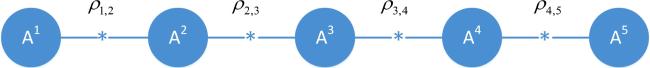
Figure 3. This chain network consists of five parties A1, A2, A3, A4 and A5, where observers Ai and Ai+1 share the quantum state ρi,i+1 (i = 1, 2, 3, 4), and observers A2, A3 and A4 perform any POVMs, respectively. |
Indeed, for convenience, in the following, write ${{\mathbb{T}}}_{m}^{n}=\sqrt{{E}_{m}^{m}}\otimes \sqrt{{E}_{m+1}^{m+1}}\otimes \cdots \otimes \sqrt{{E}_{n}^{n}}$ and, consequently, ${\left({{\mathbb{T}}}_{m}^{n}\right)}^{\dagger }={\sqrt{{E}_{m}^{m}}}^{\dagger }\otimes {\sqrt{{E}_{m+1}^{m+1}}}^{\dagger }\otimes \cdots \otimes {\sqrt{{E}_{n}^{n}}}^{\dagger }$. For ${\sigma }_{1,5}^{5}$, we have ${c}_{2}({\sigma }_{1,5}^{5})=2,{c}_{3}({\sigma }_{1,5}^{5})=2,{c}_{4}({\sigma }_{1,5}^{5})=2$ and11 ) yields
$\begin{eqnarray*}\begin{array}{l}{\sigma }_{1,5}^{5}=\displaystyle \frac{{\mathrm{Tr}}_{\mathrm{2,2},\mathrm{3,3},\mathrm{4,4}}[({I}_{1}\otimes {{\mathbb{T}}}_{2}^{4}\otimes {I}_{5})({\rho }_{\mathrm{1,2}}\otimes {\rho }_{\mathrm{2,3}}\otimes {\rho }_{\mathrm{3,4}}\otimes {\rho }_{\mathrm{4,5}})({I}_{1}\otimes {\left({{\mathbb{T}}}_{2}^{4}\right)}^{\dagger }\otimes {I}_{5})]}{\mathrm{Tr}[({I}_{1}\otimes {{\mathbb{T}}}_{2}^{4}\otimes {I}_{5})({\rho }_{\mathrm{1,2}}\otimes {\rho }_{\mathrm{2,3}}\otimes {\rho }_{\mathrm{3,4}}\otimes {\rho }_{\mathrm{4,5}})({I}_{1}\otimes {\left({{\mathbb{T}}}_{2}^{4}\right)}^{\dagger }\otimes {I}_{5})]}\\ \quad =\displaystyle \frac{{\mathrm{Tr}}_{\mathrm{4,4}}[({I}_{1}\otimes {{\mathbb{T}}}_{4}^{4}\otimes {I}_{5})(({\mathrm{Tr}}_{\mathrm{2,2},\mathrm{3,3}}[({I}_{1}\otimes {{\mathbb{T}}}_{2}^{3}\otimes {I}_{4})({\rho }_{\mathrm{1,2}}\otimes {\rho }_{\mathrm{2,3}}\otimes {\rho }_{\mathrm{3,4}})({I}_{1}\otimes {\left({{\mathbb{T}}}_{2}^{3}\right)}^{\dagger }\otimes {I}_{4})])\otimes {\rho }_{\mathrm{4,5}})({I}_{1}\otimes {\left({{\mathbb{T}}}_{4}^{4}\right)}^{\dagger }\otimes {I}_{5})]}{\mathrm{Tr}[({I}_{1}\otimes {{\mathbb{T}}}_{4}^{4}\otimes {I}_{5})(({\mathrm{Tr}}_{\mathrm{2,2},\mathrm{3,3}}[({I}_{1}\otimes {{\mathbb{T}}}_{2}^{3}\otimes {I}_{4})({\rho }_{\mathrm{1,2}}\otimes {\rho }_{\mathrm{2,3}}\otimes {\rho }_{\mathrm{3,4}})({I}_{1}\otimes {\left({{\mathbb{T}}}_{2}^{3}\right)}^{\dagger }\otimes {I}_{4})])\otimes {\rho }_{\mathrm{4,5}})({I}_{1}\otimes {\left({{\mathbb{T}}}_{4}^{4}\right)}^{\dagger }\otimes {I}_{5})]}\\ \quad =\displaystyle \frac{{\mathrm{Tr}}_{\mathrm{4,4}}[({I}_{1}\otimes {{\mathbb{T}}}_{4}^{4}\otimes {I}_{5})\left(\tfrac{{\mathrm{Tr}}_{\mathrm{2,2},\mathrm{3,3}}[({I}_{1}\otimes {{\mathbb{T}}}_{2}^{3}\otimes {I}_{4})({\rho }_{\mathrm{1,2}}\otimes {\rho }_{\mathrm{2,3}}\otimes {\rho }_{\mathrm{3,4}})({I}_{1}\otimes {\left({{\mathbb{T}}}_{2}^{3}\right)}^{\dagger }\otimes {I}_{4})]}{\mathrm{Tr}[({I}_{1}\otimes {{\mathbb{T}}}_{2}^{3}\otimes {I}_{4})({\rho }_{\mathrm{1,2}}\otimes {\rho }_{\mathrm{2,3}}\otimes {\rho }_{\mathrm{3,4}})({I}_{1}\otimes {\left({{\mathbb{T}}}_{2}^{3}\right)}^{\dagger }\otimes {I}_{4})]}\otimes {\rho }_{\mathrm{4,5}}\right)({I}_{1}\otimes {\left({{\mathbb{T}}}_{4}^{4}\right)}^{\dagger }\otimes {I}_{5})]}{\mathrm{Tr}[({I}_{1}\otimes {{\mathbb{T}}}_{4}^{4}\otimes {I}_{5})\left(\tfrac{{\mathrm{Tr}}_{\mathrm{2,2},\mathrm{3,3}}[\left({I}_{1}\otimes {{\mathbb{T}}}_{2}^{3}\otimes {I}_{4}\right)\left({\rho }_{\mathrm{1,2}}\otimes {\rho }_{\mathrm{2,3}}\otimes {\rho }_{\mathrm{3,4}}\right)\left({I}_{1}\otimes {\left({{\mathbb{T}}}_{2}^{3}\right)}^{\dagger }\otimes {I}_{4}\right)]}{\mathrm{Tr}[({I}_{1}\otimes {{\mathbb{T}}}_{2}^{3}\otimes {I}_{4})({\rho }_{\mathrm{1,2}}\otimes {\rho }_{\mathrm{2,3}}\otimes {\rho }_{\mathrm{3,4}})({I}_{1}\otimes {\left({{\mathbb{T}}}_{2}^{3}\right)}^{\dagger }\otimes {I}_{4})]}\otimes {\rho }_{\mathrm{4,5}}\right)({I}_{1}\otimes {\left({{\mathbb{T}}}_{4}^{4}\right)}^{\dagger }\otimes {I}_{5})]}\\ \quad =\displaystyle \frac{{\mathrm{Tr}}_{\mathrm{4,4}}[({I}_{1}\otimes {{\mathbb{T}}}_{4}^{4}\otimes {I}_{5})({\sigma }_{1,4}^{4}\otimes {\rho }_{\mathrm{4,5}})({I}_{1}\otimes {\left({{\mathbb{T}}}_{4}^{4}\right)}^{\dagger }\otimes {I}_{5})]}{\mathrm{Tr}[({I}_{1}\otimes {{\mathbb{T}}}_{4}^{4}\otimes {I}_{5})({\sigma }_{1,4}^{4}\otimes {\rho }_{\mathrm{4,5}})({I}_{1}\otimes {\left({{\mathbb{T}}}_{4}^{4}\right)}^{\dagger }\otimes {I}_{5})]}.\end{array}\end{eqnarray*}$
Note that $\begin{eqnarray}\begin{array}{l}{\sigma }_{1,4}^{4}=\displaystyle \frac{{\mathrm{Tr}}_{\mathrm{2,2},\mathrm{3,3}}[({I}_{1}\otimes {{\mathbb{T}}}_{2}^{3}\otimes {I}_{4})({\rho }_{\mathrm{1,2}}\otimes {\rho }_{\mathrm{2,3}}\otimes {\rho }_{\mathrm{3,4}})({I}_{1}\otimes {\left({{\mathbb{T}}}_{2}^{3}\right)}^{\dagger }\otimes {I}_{4})]}{\mathrm{Tr}[({I}_{1}\otimes {{\mathbb{T}}}_{2}^{3}\otimes {I}_{4})({\rho }_{\mathrm{1,2}}\otimes {\rho }_{\mathrm{2,3}}\otimes {\rho }_{\mathrm{3,4}})({I}_{1}\otimes {\left({{\mathbb{T}}}_{2}^{3}\right)}^{\dagger }\otimes {I}_{4})]}\\ \quad =\displaystyle \frac{{\mathrm{Tr}}_{\mathrm{3,3}}[({I}_{1}\otimes {{\mathbb{T}}}_{3}^{3}\otimes {I}_{4})(({\mathrm{Tr}}_{\mathrm{2,2}}[({I}_{1}\otimes {{\mathbb{T}}}_{2}^{2}\otimes {I}_{3})({\rho }_{\mathrm{1,2}}\otimes {\rho }_{\mathrm{2,3}})({I}_{1}\otimes {\left({{\mathbb{T}}}_{2}^{2}\right)}^{\dagger }\otimes {I}_{3})])\otimes {\rho }_{\mathrm{3,4}})({I}_{1}\otimes {\left({{\mathbb{T}}}_{3}^{3}\right)}^{\dagger }\otimes {I}_{4})]}{\mathrm{Tr}[({I}_{1}\otimes {{\mathbb{T}}}_{3}^{3}\otimes {I}_{4})(({\mathrm{Tr}}_{\mathrm{2,2}}[({I}_{1}\otimes {{\mathbb{T}}}_{2}^{2}\otimes {I}_{3})({\rho }_{\mathrm{1,2}}\otimes {\rho }_{\mathrm{2,3}})({I}_{1}\otimes {\left({{\mathbb{T}}}_{2}^{2}\right)}^{\dagger }\otimes {I}_{3})])\otimes {\rho }_{\mathrm{3,4}})({I}_{1}\otimes {\left({{\mathbb{T}}}_{3}^{3}\right)}^{\dagger }\otimes {I}_{4})]}\\ \quad =\displaystyle \frac{{\mathrm{Tr}}_{\mathrm{3,3}}[({I}_{1}\otimes {{\mathbb{T}}}_{3}^{3}\otimes {I}_{4})\left(\tfrac{{\mathrm{Tr}}_{\mathrm{2,2}}[({I}_{1}\otimes {{\mathbb{T}}}_{2}^{2}\otimes {I}_{3})({\rho }_{\mathrm{1,2}}\otimes {\rho }_{\mathrm{2,3}})({I}_{1}\otimes {\left({{\mathbb{T}}}_{2}^{2}\right)}^{\dagger }\otimes {I}_{3})]}{\mathrm{Tr}[({I}_{1}\otimes {{\mathbb{T}}}_{2}^{2}\otimes {I}_{3})({\rho }_{\mathrm{1,2}}\otimes {\rho }_{\mathrm{2,3}})({I}_{1}\otimes {\left({{\mathbb{T}}}_{2}^{2}\right)}^{\dagger }\otimes {I}_{3})]}\otimes {\rho }_{\mathrm{3,4}}\right)({I}_{1}\otimes {\left({{\mathbb{T}}}_{3}^{3}\right)}^{\dagger }\otimes {I}_{4})]}{\mathrm{Tr}[({I}_{1}\otimes {{\mathbb{T}}}_{3}^{3}\otimes {I}_{4})\left(\tfrac{{\mathrm{Tr}}_{\mathrm{2,2}}[\left({I}_{1}\otimes {{\mathbb{T}}}_{2}^{2}\otimes {I}_{3}\right)\left({\rho }_{\mathrm{1,2}}\otimes {\rho }_{\mathrm{2,3}}\right)\left({I}_{1}\otimes {\left({{\mathbb{T}}}_{2}^{2}\right)}^{\dagger }\otimes {I}_{3}\right)]}{\mathrm{Tr}[({I}_{1}\otimes {{\mathbb{T}}}_{2}^{2}\otimes {I}_{3})({\rho }_{\mathrm{1,2}}\otimes {\rho }_{\mathrm{2,3}})({I}_{1}\otimes {\left({{\mathbb{T}}}_{2}^{2}\right)}^{\dagger }\otimes {I}_{3})]}\otimes {\rho }_{\mathrm{3,4}}\right)({I}_{1}\otimes {\left({{\mathbb{T}}}_{3}^{3}\right)}^{\dagger }\otimes {I}_{4})]}\\ \quad =\displaystyle \frac{{\mathrm{Tr}}_{\mathrm{3,3}}[({I}_{1}\otimes {{\mathbb{T}}}_{3}^{3}\otimes {I}_{4})({\sigma }_{1,3}^{3}\otimes {\rho }_{\mathrm{3,4}})({I}_{1}\otimes {\left({{\mathbb{T}}}_{3}^{3}\right)}^{\dagger }\otimes {I}_{4})]}{\mathrm{Tr}[({I}_{1}\otimes {{\mathbb{T}}}_{3}^{3}\otimes {I}_{4})({\sigma }_{1,3}^{3}\otimes {\rho }_{\mathrm{3,4}})({I}_{1}\otimes {\left({{\mathbb{T}}}_{3}^{3}\right)}^{\dagger }\otimes {I}_{4})]},\end{array}\end{eqnarray}$
and $\begin{eqnarray*}{\sigma }_{1,3}^{3}=\displaystyle \frac{{\mathrm{Tr}}_{\mathrm{2,2}}[({I}_{1}\otimes \sqrt{{E}_{2}^{2}}\otimes {I}_{3})({\rho }_{\mathrm{1,2}}\otimes {\rho }_{\mathrm{2,3}})({I}_{1}\otimes {\sqrt{{E}_{2}^{2}}}^{\dagger }\otimes {I}_{3})]}{\mathrm{Tr}[({I}_{1}\otimes \sqrt{{E}_{2}^{2}}\otimes {I}_{3})({\rho }_{\mathrm{1,2}}\otimes {\rho }_{\mathrm{2,3}})({I}_{1}\otimes {\sqrt{{E}_{2}^{2}}}^{\dagger }\otimes {I}_{3})]}.\end{eqnarray*}$
As $\begin{eqnarray*}\begin{array}{l}\sqrt{{E}_{2}^{2}}={\sqrt{{E}_{2}^{2}}}^{\dagger }=\displaystyle \frac{\left(\sqrt{\tfrac{1+3{\lambda }_{2}}{4}}-\sqrt{\tfrac{1-{\lambda }_{2}}{4}}\right)}{2}\\ \quad \times (| 00\rangle \langle 00| -| 00\rangle \langle 11| -| 11\rangle \langle 00| +| 11\rangle \langle 11| )\\ \quad +\sqrt{\displaystyle \frac{1-{\lambda }_{2}}{4}}(| 00\rangle \langle 00| \\ \quad +| 01\rangle \langle 01| +| 10\rangle \langle 10| +| 11\rangle \langle 11| ),\end{array}\end{eqnarray*}$
and $\begin{eqnarray*}\begin{array}{l}{\rho }_{\mathrm{1,2}}\otimes {\rho }_{\mathrm{2,3}}=\displaystyle \frac{1}{4}(| 0000\rangle \langle 0000| \\ \quad -| 0000\rangle \langle 0011| -| 0011\rangle \langle 0000| +| 0011\rangle \langle 0011| \\ \quad +| 0000\rangle \langle 1100| -| 0000\rangle \langle 1111| \\ \quad -| 0011\rangle \langle 1100| +| 0011\rangle \langle 1111| \\ \quad +| 1100\rangle \langle 0000| -| 1100\rangle \langle 0011| \\ \quad -| 1111\rangle \langle 0000| +| 1111\rangle \langle 0011| \\ \quad +| 1100\rangle \langle 1100| -| 1100\rangle \langle 1111| \\ \quad -| 1111\rangle \langle 1100| +| 1111\rangle \langle 1111| ),\end{array}\end{eqnarray*}$
a direct calculation gives $\begin{eqnarray*}\begin{array}{l}\mathrm{Tr}[({I}_{1}\otimes \sqrt{{E}_{2}^{2}}\otimes {I}_{3})({\rho }_{\mathrm{1,2}}\otimes {\rho }_{\mathrm{2,3}})\\ \quad \times ({I}_{1}\otimes {\sqrt{{E}_{2}^{2}}}^{\dagger }\otimes {I}_{3})]=\displaystyle \frac{1}{4},\end{array}\end{eqnarray*}$
and $\begin{eqnarray*}\begin{array}{l}{\mathrm{Tr}}_{\mathrm{2,2}}[({I}_{1}\otimes \sqrt{{E}_{2}^{2}}\otimes {I}_{3})({\rho }_{\mathrm{1,2}}\otimes {\rho }_{\mathrm{2,3}})\\ \quad \times ({I}_{1}\otimes {\sqrt{{E}_{2}^{2}}}^{\dagger }\otimes {I}_{3})]=\displaystyle \frac{{\lambda }_{2}}{4}| {\psi }_{1}\rangle \langle {\psi }_{1}| +\displaystyle \frac{1-{\lambda }_{2}}{16}{{\mathbb{I}}}_{4}.\end{array}\end{eqnarray*}$
So $\begin{eqnarray*}{\sigma }_{1,3}^{3}={\lambda }_{2}| {\psi }_{1}\rangle \langle {\psi }_{1}| +\displaystyle \frac{1-{\lambda }_{2}}{4}{{\mathbb{I}}}_{4}.\end{eqnarray*}$
Replacing the above equation into equation ( $\begin{eqnarray*}{\sigma }_{1,4}^{4}={\lambda }_{2}{\lambda }_{3}| {\psi }_{1}\rangle \langle {\psi }_{1}| +\displaystyle \frac{1-{\lambda }_{2}{\lambda }_{3}}{4}{{\mathbb{I}}}_{4};\end{eqnarray*}$
and replacing this into the formula of ${\sigma }_{1,5}^{5}$, one obtains $\begin{eqnarray*}{\sigma }_{1,5}^{5}={\lambda }_{2}{\lambda }_{3}{\lambda }_{4}| {\psi }_{1}\rangle \langle {\psi }_{1}| +\displaystyle \frac{1-{\lambda }_{2}{\lambda }_{3}{\lambda }_{4}}{4}{{\mathbb{I}}}_{4}.\end{eqnarray*}$
Similar to the above discussion, one can obtain expressions of ${\sigma }_{1,4}^{5}$, ${\sigma }_{2,4}^{5}$, ${\sigma }_{2,5}^{5}$, ${\sigma }_{3,4}^{5}$, ${\sigma }_{3,5}^{5}$, ${\sigma }_{4,5}^{5}$.
Next, consider ${\sigma }_{1,2}^{5}$. We first show that ${\sigma }_{1,2}^{5}={\sigma }_{1,2}^{4}={\sigma }_{1,2}^{3}$. In fact, take any orthonormal bases {e1, e2} of H2,1 and {f1, f2} of H2,2, and write Eij = ei ⨂ ej and Fij = fi ⨂ fj. Then, $\sqrt{{E}_{2}^{2}}$ can be written as
$\begin{eqnarray*}\begin{array}{l}\sqrt{{E}_{2}^{2}}=\displaystyle \sum _{i,j=1;k,l=1}{t}_{{ij},{kl}}{E}_{{ij}}\otimes {F}_{{kl}}\\ \,=\,\displaystyle \sum _{i,j=1}{E}_{{ij}}\otimes \displaystyle \sum _{k,l=1}{t}_{{ij},{kl}}{F}_{{kl}}.\end{array}\end{eqnarray*}$
Let ${\mathbb{E}}={\sum }_{i,j=1}{E}_{{ij}}$ and ${\mathbb{F}}={\sum }_{k,l=1}{t}_{{ij},{kl}}{F}_{{kl}}$. A routine calculation gives $\begin{eqnarray*}\begin{array}{l}{\sigma }_{1,2}^{5}=\displaystyle \frac{{\mathrm{Tr}}_{\mathrm{2,3},\mathrm{3,4},\mathrm{4,5}}[({I}_{1}\otimes {{\mathbb{T}}}_{2}^{4}\otimes {I}_{5})({\rho }_{\mathrm{1,2}}\otimes {\rho }_{\mathrm{2,3}}\otimes {\rho }_{\mathrm{3,4}}\otimes {\rho }_{\mathrm{4,5}})({I}_{1}\otimes {\left({{\mathbb{T}}}_{2}^{4}\right)}^{\dagger }\otimes {I}_{5})]}{\mathrm{Tr}[({I}_{1}\otimes {{\mathbb{T}}}_{2}^{4}\otimes {I}_{5})({\rho }_{\mathrm{1,2}}\otimes {\rho }_{\mathrm{2,3}}\otimes {\rho }_{\mathrm{3,4}}\otimes {\rho }_{\mathrm{4,5}})({I}_{1}\otimes {\left({{\mathbb{T}}}_{2}^{4}\right)}^{\dagger }\otimes {I}_{5})]}\\ \quad =\displaystyle \frac{{\mathrm{Tr}}_{\mathrm{2,3},\mathrm{3,4},\mathrm{4,5}}[({I}_{1}\otimes {\mathbb{E}}\otimes {\mathbb{F}}\otimes {{\mathbb{T}}}_{3}^{4}\otimes {I}_{5})({\rho }_{\mathrm{1,2}}\otimes {\rho }_{\mathrm{2,3}}\otimes {\rho }_{\mathrm{3,4}}\otimes {\rho }_{\mathrm{4,5}})({I}_{1}\otimes {\mathbb{E}}\otimes {\mathbb{F}}\otimes {\left({{\mathbb{T}}}_{3}^{4}\right)}^{\dagger }\otimes {I}_{5})]}{\mathrm{Tr}[({I}_{1}\otimes {\mathbb{E}}\otimes {\mathbb{F}}\otimes {{\mathbb{T}}}_{3}^{4}\otimes {I}_{5})({\rho }_{\mathrm{1,2}}\otimes {\rho }_{\mathrm{2,3}}\otimes {\rho }_{\mathrm{3,4}}\otimes {\rho }_{\mathrm{4,5}})({I}_{1}\otimes {\mathbb{E}}\otimes {\mathbb{F}}\otimes {\left({{\mathbb{T}}}_{3}^{4}\right)}^{\dagger }\otimes {I}_{5})]}\\ \quad =\displaystyle \frac{\left({I}_{1}\otimes {\mathbb{E}}\right){\rho }_{\mathrm{1,2}}\left({I}_{1}\otimes {\mathbb{E}}\right)\cdot {\mathrm{Tr}}_{\mathrm{2,3},\mathrm{3,4},\mathrm{4,5}}[\left({\mathbb{F}}\otimes {{\mathbb{T}}}_{3}^{4}\otimes {I}_{5}\right)\left({\rho }_{\mathrm{2,3}}\otimes {\rho }_{\mathrm{3,4}}\otimes {\rho }_{\mathrm{4,5}}\right)\left({\mathbb{F}}\otimes {\left({{\mathbb{T}}}_{3}^{4}\right)}^{\dagger }\otimes {I}_{5}\right)]}{{\mathrm{Tr}}_{\mathrm{1,2}}[({I}_{1}\otimes {\mathbb{E}}){\rho }_{\mathrm{1,2}}({I}_{1}\otimes {\mathbb{E}})]\cdot {\mathrm{Tr}}_{\mathrm{2,3},\mathrm{3,4},\mathrm{4,5}}[({\mathbb{F}}\otimes {{\mathbb{T}}}_{3}^{4}\otimes {I}_{5})({\rho }_{\mathrm{2,3}}\otimes {\rho }_{\mathrm{3,4}}\otimes {\rho }_{\mathrm{4,5}})({\mathbb{F}}\otimes {\left({{\mathbb{T}}}_{3}^{4}\right)}^{\dagger }\otimes {I}_{5})]}\\ \quad =\displaystyle \frac{\left({I}_{1}\otimes {\mathbb{E}}\right){\rho }_{\mathrm{1,2}}({I}_{1}\otimes {\mathbb{E}})}{{\mathrm{Tr}}_{\mathrm{1,2}}[({I}_{1}\otimes {\mathbb{E}}){\rho }_{\mathrm{1,2}}({I}_{1}\otimes {\mathbb{E}})]},\end{array}\end{eqnarray*}$
$\begin{eqnarray*}\begin{array}{l}{\sigma }_{1,2}^{4}\quad =\displaystyle \frac{{\mathrm{Tr}}_{\mathrm{2,3},\mathrm{3,4}}[({I}_{1}\otimes {{\mathbb{T}}}_{2}^{3}\otimes {I}_{4})({\rho }_{\mathrm{1,2}}\otimes {\rho }_{\mathrm{2,3}}\otimes {\rho }_{\mathrm{3,4}})({I}_{1}\otimes {\left({{\mathbb{T}}}_{2}^{3}\right)}^{\dagger }\otimes {I}_{4})]}{\mathrm{Tr}[({I}_{1}\otimes {{\mathbb{T}}}_{2}^{3}\otimes {I}_{4})({\rho }_{\mathrm{1,2}}\otimes {\rho }_{\mathrm{2,3}}\otimes {\rho }_{\mathrm{3,4}})({I}_{1}\otimes {\left({{\mathbb{T}}}_{2}^{3}\right)}^{\dagger }\otimes {I}_{4})]}\\ \quad =\displaystyle \frac{{\mathrm{Tr}}_{\mathrm{2,3},\mathrm{3,4}}[({I}_{1}\otimes {\mathbb{E}}\otimes {\mathbb{F}}\otimes {{\mathbb{T}}}_{3}^{3}\otimes {I}_{4})({\rho }_{\mathrm{1,2}}\otimes {\rho }_{\mathrm{2,3}}\otimes {\rho }_{\mathrm{3,4}})({I}_{1}\otimes {\mathbb{E}}\otimes {\mathbb{F}}\otimes {\left({{\mathbb{T}}}_{3}^{3}\right)}^{\dagger }\otimes {I}_{4})]}{\mathrm{Tr}[({I}_{1}\otimes {\mathbb{E}}\otimes {\mathbb{F}}\otimes {{\mathbb{T}}}_{3}^{3}\otimes {I}_{4})({\rho }_{\mathrm{1,2}}\otimes {\rho }_{\mathrm{2,3}}\otimes {\rho }_{\mathrm{3,4}})({I}_{1}\otimes {\mathbb{E}}\otimes {\mathbb{F}}\otimes {\left({{\mathbb{T}}}_{3}^{3}\right)}^{\dagger }\otimes {I}_{4})]}\\ \quad =\displaystyle \frac{\left({I}_{1}\otimes {\mathbb{E}}\right){\rho }_{\mathrm{1,2}}\left({I}_{1}\otimes {\mathbb{E}}\right)\cdot {\mathrm{Tr}}_{\mathrm{2,3},\mathrm{3,4}}[\left({\mathbb{F}}\otimes {{\mathbb{T}}}_{3}^{3}\otimes {I}_{4}\right)\left({\rho }_{\mathrm{2,3}}\otimes {\rho }_{\mathrm{3,4}}\right)\left({\mathbb{F}}\otimes {\left({{\mathbb{T}}}_{3}^{3}\right)}^{\dagger }\otimes {I}_{4}\right)]}{{\mathrm{Tr}}_{\mathrm{1,2}}[({I}_{1}\otimes {\mathbb{E}}){\rho }_{\mathrm{1,2}}({I}_{1}\otimes {\mathbb{E}})]\cdot {\mathrm{Tr}}_{\mathrm{2,3},\mathrm{3,4}}[({\mathbb{F}}\otimes {{\mathbb{T}}}_{3}^{3}\otimes {I}_{4})({\rho }_{\mathrm{2,3}}\otimes {\rho }_{\mathrm{3,4}})({\mathbb{F}}\otimes {\left({{\mathbb{T}}}_{3}^{3}\right)}^{\dagger }\otimes {I}_{4})]}\\ \quad =\displaystyle \frac{\left({I}_{1}\otimes {\mathbb{E}}\right){\rho }_{\mathrm{1,2}}({I}_{1}\otimes {\mathbb{E}})}{{\mathrm{Tr}}_{\mathrm{1,2}}[({I}_{1}\otimes {\mathbb{E}}){\rho }_{\mathrm{1,2}}({I}_{1}\otimes {\mathbb{E}})]},\end{array}\end{eqnarray*}$
and $\begin{eqnarray*}\begin{array}{l}{\sigma }_{1,2}^{3}=\displaystyle \frac{{\mathrm{Tr}}_{\mathrm{2,3}}[\left({I}_{1}\otimes \sqrt{{E}_{2}^{2}}\otimes {I}_{3}\right)\left({\rho }_{\mathrm{1,2}}\otimes {\rho }_{\mathrm{2,3}}\right)\left({I}_{1}\otimes {\sqrt{{E}_{2}^{2}}}^{\dagger }\otimes {I}_{3}\right)]}{\mathrm{Tr}[({I}_{1}\otimes \sqrt{{E}_{2}^{2}}\otimes {I}_{3})({\rho }_{\mathrm{1,2}}\otimes {\rho }_{\mathrm{2,3}})({I}_{1}\otimes {\sqrt{{E}_{2}^{2}}}^{\dagger }\otimes {I}_{3})]}\\ \quad =\displaystyle \frac{{\mathrm{Tr}}_{\mathrm{2,3}}[\left({I}_{1}\otimes {\mathbb{E}}\otimes {\mathbb{F}}\otimes {I}_{3}\right)\left({\rho }_{\mathrm{1,2}}\otimes {\rho }_{\mathrm{2,3}}\right)\left({I}_{1}\otimes {\mathbb{E}}\otimes {\mathbb{F}}\otimes {I}_{3}\right)]}{\mathrm{Tr}[({I}_{1}\otimes {\mathbb{E}}\otimes {\mathbb{F}}\otimes {I}_{3})({\rho }_{\mathrm{1,2}}\otimes {\rho }_{\mathrm{2,3}})({I}_{1}\otimes {\mathbb{E}}\otimes {\mathbb{F}}\otimes {I}_{3})]}\\ \quad =\displaystyle \frac{\left({I}_{1}\otimes {\mathbb{E}}\right){\rho }_{\mathrm{1,2}}\left({I}_{1}\otimes {\mathbb{E}}\right)\cdot {\mathrm{Tr}}_{\mathrm{2,3}}[\left({\mathbb{F}}\otimes {I}_{3}\right){\rho }_{\mathrm{2,3}}\left({\mathbb{F}}\otimes {I}_{3}\right)]}{{\mathrm{Tr}}_{\mathrm{1,2}}[({I}_{1}\otimes {\mathbb{E}}){\rho }_{\mathrm{1,2}}({I}_{1}\otimes {\mathbb{E}})]\cdot {\mathrm{Tr}}_{\mathrm{2,3}}[({\mathbb{F}}\otimes {I}_{3}){\rho }_{\mathrm{2,3}}({\mathbb{F}}\otimes {I}_{3})]}\\ \,=\displaystyle \frac{\left({I}_{1}\otimes {\mathbb{E}}\right){\rho }_{\mathrm{1,2}}({I}_{1}\otimes {\mathbb{E}})}{{\mathrm{Tr}}_{\mathrm{1,2}}[({I}_{1}\otimes {\mathbb{E}}){\rho }_{\mathrm{1,2}}({I}_{1}\otimes {\mathbb{E}})]},\end{array}\end{eqnarray*}$
which implies that ${\sigma }_{1,2}^{5}={\sigma }_{1,2}^{4}={\sigma }_{1,2}^{3}$. Note that $\begin{eqnarray*}{\sigma }_{1,2}^{3}=\displaystyle \frac{{\mathrm{Tr}}_{\mathrm{2,3}}[({I}_{1}\otimes \sqrt{{E}_{2}^{2}}\otimes {I}_{3})({\rho }_{\mathrm{1,2}}\otimes {\rho }_{\mathrm{2,3}})({I}_{1}\otimes {\sqrt{{E}_{2}^{2}}}^{\dagger }\otimes {I}_{3})]}{\mathrm{Tr}[({I}_{1}\otimes \sqrt{{E}_{2}^{2}}\otimes {I}_{3})({\rho }_{\mathrm{1,2}}\otimes {\rho }_{\mathrm{2,3}})({I}_{1}\otimes {\sqrt{{E}_{2}^{2}}}^{\dagger }\otimes {I}_{3})]},\end{eqnarray*}$
and $\begin{eqnarray*}\begin{array}{l}{\mathrm{Tr}}_{\mathrm{2,3}}[({I}_{1}\otimes \sqrt{{E}_{2}^{2}}\otimes {I}_{3})({\rho }_{\mathrm{1,2}}\otimes {\rho }_{\mathrm{2,3}})({I}_{1}\otimes {\sqrt{{E}_{2}^{2}}}^{\dagger }\otimes {I}_{3})]\\ \quad =\displaystyle \frac{s({\lambda }_{2})}{4}| {\psi }_{1}\rangle \langle {\psi }_{1}| +\displaystyle \frac{1-s({\lambda }_{2})}{16}{{\mathbb{I}}}_{4}.\end{array}\end{eqnarray*}$
It follows that $\begin{eqnarray*}{\sigma }_{1,2}^{3}=s({\lambda }_{2})| {\psi }_{1}\rangle \langle {\psi }_{1}| +\displaystyle \frac{1-s({\lambda }_{2})}{4}{{\mathbb{I}}}_{4}.\end{eqnarray*}$
Hence $\begin{eqnarray*}{\sigma }_{1,2}^{5}={\sigma }_{1,2}^{4}={\sigma }_{1,2}^{3}=s({\lambda }_{2})| {\psi }_{1}\rangle \langle {\psi }_{1}| +\displaystyle \frac{1-s({\lambda }_{2})}{4}{{\mathbb{I}}}_{4}.\end{eqnarray*}$
Using a similar argument to that of ${\sigma }_{1,2}^{5}$, one can show that
$\begin{eqnarray*}\begin{array}{l}{\sigma }_{1,3}^{5}={\sigma }_{1,3}^{4}={\lambda }_{2}s({\lambda }_{3})| {\psi }_{1}\rangle \langle {\psi }_{1}| \\ \quad +\displaystyle \frac{1-{\lambda }_{2}s({\lambda }_{3})}{4}{{\mathbb{I}}}_{4},\end{array}\end{eqnarray*}$
$\begin{eqnarray*}\begin{array}{l}{\sigma }_{2,3}^{5}={\sigma }_{2,3}^{4}=s({\lambda }_{2})s({\lambda }_{3})| {\psi }_{2}\rangle \langle {\psi }_{2}| \\ \quad +\displaystyle \frac{1-s\left({\lambda }_{2}\right)s({\lambda }_{3})}{4}{{\mathbb{I}}}_{4}.\end{array}\end{eqnarray*}$
4. Quantum correlations in chain network
With the forms of all post-measurement states ${\sigma }_{p,q}^{n}(\vec{{\boldsymbol{u}}},\vec{{\boldsymbol{v}}})$ in section 3 , we will examine their Bell nonlocality, steerability and entanglement in this section. For simplicity, assume that each Ak (k ∈ {2,…,n − 1}) respectively performs the POVM of equation (5 ) with the same parameter, i.e. λ2 = ⋯ = λn−1 = λ. Then, all post-measurement states ${\sigma }_{p,q}^{n}(\vec{{\boldsymbol{u}}},\vec{{\boldsymbol{v}}})$ have the forms of equation (8 ). For convenience, in the sequel, write ${\sigma }_{p,q}^{n}={\sigma }_{p,q}^{n}(\vec{{\boldsymbol{u}}},\vec{{\boldsymbol{v}}})$. Through calculations, we derive that the eigenvalues of ${R}_{{\sigma }_{p,q}^{n}}^{\dagger }{R}_{{\sigma }_{p,q}^{n}}$ are2 )–(4 ), one gets
In the following, we will explicitly examine the quantifications of Bell nonlocality, EPR steering and entanglement of all post-measurement states for n = 5 with the measurement strategy equations (9 )–(10 ) by plotting these correlation functions with respect to parameter λ, respectively. In addition, we compare the quantifications of these three correlations for some specific post-measurement states.
$\begin{eqnarray*}\begin{array}{rcl}{t}_{1} & = & {\left[s{\left(\lambda \right)}^{2}{\lambda }^{q-p-1}\right]}^{2},\\ {t}_{2} & = & {\left[s{\left(\lambda \right)}^{2}{\lambda }^{q-p-1}\right]}^{2},\\ {t}_{3} & = & {\left[s{\left(\lambda \right)}^{2}{\lambda }^{q-p-1}\right]}^{2};\end{array}\end{eqnarray*}$
and the minimum eigenvalue of ${\left({\sigma }_{p,q}^{n}\right)}^{{T}_{B}}$ is $\mu =\tfrac{1-3s{\left(\lambda \right)}^{2}{\lambda }^{q-p-1}}{4}$. According to equations ( $\begin{eqnarray*}\begin{array}{rcl}{ \mathcal N }({\sigma }_{p,q}^{n}) & = & \max \left\{0,\displaystyle \frac{\sqrt{2}s{\left(\lambda \right)}^{2}{\lambda }^{q-p-1}-1}{\sqrt{2}-1}\right\},\\ { \mathcal S }({\sigma }_{p,q}^{n}) & = & \max \left\{0,\displaystyle \frac{\sqrt{3}s{\left(\lambda \right)}^{2}{\lambda }^{q-p-1}-1}{\sqrt{3}-1}\right\},\end{array}\end{eqnarray*}$
and $\begin{eqnarray*}{ \mathcal E }({\sigma }_{p,q}^{n})=2\max \left\{0,\displaystyle \frac{3s{\left(\lambda \right)}^{2}{\lambda }^{q-p-1}-1}{4}\right\},\end{eqnarray*}$
where $s(\lambda )=\tfrac{1}{2}[1-\lambda +\sqrt{(1-\lambda )(1+3\lambda )}]$ when p ≠ 1 and q ≠ n; s(λ) = 1 when p = 1 or q = n. Hence, we obtain the following results:| (1) If $\tfrac{1}{\sqrt{2}}\lt s{\left(\lambda \right)}^{2}{\lambda }^{q-p-1}\leqslant 1$, then ${\sigma }_{p,q}^{n}$ is Bell nonlocal. | |
| (2) If $\tfrac{1}{\sqrt{3}}\lt s{\left(\lambda \right)}^{2}{\lambda }^{q-p-1}\leqslant 1$, then ${\sigma }_{p,q}^{n}$ is EPR steerable. | |
| (3) If $\tfrac{1}{3}\lt s{\left(\lambda \right)}^{2}{\lambda }^{q-p-1}\leqslant 1$, then ${\sigma }_{p,q}^{n}$ is entangled. |
Note that, in this circumstance, all the post-measurement states are
$\begin{eqnarray*}\left\{\begin{array}{ll}{\sigma }_{1,2}^{5}=s(\lambda )| {\psi }_{1}\rangle \langle {\psi }_{1}| +\displaystyle \frac{1-s(\lambda )}{4}{{\mathbb{I}}}_{4}, & {\sigma }_{1,3}^{5}=\lambda s(\lambda )| {\psi }_{1}\rangle \langle {\psi }_{1}| +\displaystyle \frac{1-\lambda s(\lambda )}{4}{{\mathbb{I}}}_{4},\\ {\sigma }_{1,4}^{5}={\lambda }^{2}s(\lambda )| {\psi }_{1}\rangle \langle {\psi }_{1}| +\displaystyle \frac{1-{\lambda }^{2}s(\lambda )}{4}{{\mathbb{I}}}_{4}, & {\sigma }_{1,5}^{5}={\lambda }^{3}| {\psi }_{1}\rangle \langle {\psi }_{1}| +\displaystyle \frac{1-{\lambda }^{3}}{4}{{\mathbb{I}}}_{4},\\ {\sigma }_{2,3}^{5}=s{\left(\lambda \right)}^{2}| {\psi }_{2}\rangle \langle {\psi }_{2}| +\displaystyle \frac{1-s{\left(\lambda \right)}^{2}}{4}{{\mathbb{I}}}_{4}, & {\sigma }_{2,4}^{5}=\lambda s{\left(\lambda \right)}^{2}| {\psi }_{2}\rangle \langle {\psi }_{2}| +\displaystyle \frac{1-\lambda s{\left(\lambda \right)}^{2}}{4}{{\mathbb{I}}}_{4},\\ {\sigma }_{2,5}^{5}={\lambda }^{2}s(\lambda )| {\psi }_{2}\rangle \langle {\psi }_{2}| +\displaystyle \frac{1-{\lambda }^{2}s(\lambda )}{4}{{\mathbb{I}}}_{4}, & {\sigma }_{3,4}^{5}=s{\left(\lambda \right)}^{2}| {\psi }_{3}\rangle \langle {\psi }_{3}| +\displaystyle \frac{1-s{\left(\lambda \right)}^{2}}{4}{{\mathbb{I}}}_{4},\\ {\sigma }_{3,5}^{5}=\lambda s(\lambda )| {\psi }_{3}\rangle \langle {\psi }_{3}| +\displaystyle \frac{1-\lambda s(\lambda )}{4}{{\mathbb{I}}}_{4}, & {\sigma }_{4,5}^{5}=s(\lambda )| {\psi }_{4}\rangle \langle {\psi }_{4}| +\displaystyle \frac{1-s(\lambda )}{4}{{\mathbb{I}}}_{4},\end{array}\right.\end{eqnarray*}$
where $s(\lambda )=\tfrac{1}{2}[1-\lambda +\sqrt{(1-\lambda )(1+3\lambda )}]$. Therefore, we can obtain the singular values of the CMs of these post-measurement states: $\begin{eqnarray}\left\{\begin{array}{l}\sigma ({R}_{{\sigma }_{1,5}^{5}}^{\dagger }{R}_{{\sigma }_{\mathrm{1,5}}^{5}})=\{{\lambda }^{6},{\lambda }^{6},{\lambda }^{6}\},\\ \sigma ({R}_{{\sigma }_{2,4}^{5}}^{\dagger }{R}_{{\sigma }_{\mathrm{2,4}}^{5}})=\{{\lambda }^{2}s{\left(\lambda \right)}^{4},{\lambda }^{2}s{\left(\lambda \right)}^{4},{\lambda }^{2}s{\left(\lambda \right)}^{4}\},\\ \sigma ({R}_{{\sigma }_{1,2}^{5}}^{\dagger }{R}_{{\sigma }_{\mathrm{1,2}}^{5}})=\sigma ({R}_{{\sigma }_{4,5}^{5}}^{\dagger }{R}_{{\sigma }_{\mathrm{4,5}}^{5}})=\{s{\left(\lambda \right)}^{2},s{\left(\lambda \right)}^{2},s{\left(\lambda \right)}^{2}\},\\ \sigma ({R}_{{\sigma }_{1,3}^{5}}^{\dagger }{R}_{{\sigma }_{\mathrm{1,3}}^{5}})=\sigma ({R}_{{\sigma }_{3,5}^{5}}^{\dagger }{R}_{{\sigma }_{\mathrm{3,5}}^{5}})=\{{\lambda }^{2}s{\left(\lambda \right)}^{2},{\lambda }^{2}s{\left(\lambda \right)}^{2},{\lambda }^{2}s{\left(\lambda \right)}^{2}\},\\ \sigma ({R}_{{\sigma }_{1,4}^{5}}^{\dagger }{R}_{{\sigma }_{\mathrm{1,4}}^{5}})=\sigma ({R}_{{\sigma }_{2,5}^{5}}^{\dagger }{R}_{{\sigma }_{\mathrm{2,5}}^{5}})=\{{\lambda }^{4}s{\left(\lambda \right)}^{2},{\lambda }^{4}s{\left(\lambda \right)}^{2},{\lambda }^{4}s{\left(\lambda \right)}^{2}\},\\ \sigma ({R}_{{\sigma }_{2,3}^{5}}^{\dagger }{R}_{{\sigma }_{\mathrm{2,3}}^{5}})=\sigma ({R}_{{\sigma }_{3,4}^{5}}^{\dagger }{R}_{{\sigma }_{\mathrm{3,4}}^{5}})=\{s{\left(\lambda \right)}^{4},s{\left(\lambda \right)}^{4},s{\left(\lambda \right)}^{4}\}.\end{array}\right.\end{eqnarray}$
4.1. Bell nonlocality
We firstly focus on the quantification of Bell nonlocality of the post-measurement states in the network of figure 3. From equations (2 ) and (12 ), we know that
$\begin{eqnarray*}\begin{array}{l}{ \mathcal N }({\sigma }_{1,5}^{5})=\max \left\{0,\displaystyle \frac{\sqrt{2}{\lambda }^{3}-1}{\sqrt{2}-1}\right\},\\ { \mathcal N }({\sigma }_{1,2}^{5})={ \mathcal N }({\sigma }_{4,5}^{5})=\max \left\{0,\displaystyle \frac{\sqrt{2}s(\lambda )-1}{\sqrt{2}-1}\right\},\end{array}\end{eqnarray*}$
$\begin{eqnarray*}\begin{array}{l}{ \mathcal N }({\sigma }_{1,3}^{5})={ \mathcal N }({\sigma }_{3,5}^{5})=\max \left\{0,\displaystyle \frac{\sqrt{2}\lambda s(\lambda )-1}{\sqrt{2}-1}\right\},\\ { \mathcal N }({\sigma }_{1,4}^{5})={ \mathcal N }({\sigma }_{2,5}^{5})=\max \left\{0,\displaystyle \frac{\sqrt{2}{\lambda }^{2}s(\lambda )-1}{\sqrt{2}-1}\right\},\end{array}\end{eqnarray*}$
$\begin{eqnarray*}\begin{array}{l}{ \mathcal N }({\sigma }_{2,3}^{5})={ \mathcal N }({\sigma }_{3,4}^{5})=\max \left\{0,\displaystyle \frac{\sqrt{2}s{\left(\lambda \right)}^{2}-1}{\sqrt{2}-1}\right\},\\ { \mathcal N }({\sigma }_{2,4}^{5})=\max \left\{0,\displaystyle \frac{\sqrt{2}\lambda s{\left(\lambda \right)}^{2}-1}{\sqrt{2}-1}\right\}.\end{array}\end{eqnarray*}$
From figure 4, we can see that in the five-parties chain network, the post-measurement states ${\sigma }_{1,3}^{5}$, ${\sigma }_{3,5}^{5}$, ${\sigma }_{1,4}^{5}$, ${\sigma }_{2,5}^{5}$ and ${\sigma }_{2,4}^{5}$ are not Bell nonlocal. For the post-measurement states ${\sigma }_{2,3}^{5}$ and ${\sigma }_{3,4}^{5}$, they are Bell nonlocal when 0 < λ < 0.45; ${ \mathcal N }({\sigma }_{2,3}^{5})={ \mathcal N }({\sigma }_{3,4}^{5})$ gradually decreases as the parameter λ gradually increases; and ${ \mathcal N }({\sigma }_{2,3}^{5})={ \mathcal N }({\sigma }_{3,4}^{5})=0$ for 1 ≥ λ ≥ 0.45, i.e. the Bell nonlocality of ${\sigma }_{2,3}^{5}$ and ${\sigma }_{3,4}^{5}$ disappears. For the post-measurement states ${\sigma }_{1,2}^{5}$ and ${\sigma }_{4,5}^{5}$, when 0 < λ < 0.62, they are Bell nonlocal, and when 0.62 ≤ λ ≤ 1, the Bell nonlocality of ${\sigma }_{1,2}^{5}$ and ${\sigma }_{4,5}^{5}$ disappears. In contrast, when 0 < λ < 0.89, the post-measurement state ${\sigma }_{1,5}^{5}$ is Bell local, and when 0.89 < λ ≤ 1, $0\lt { \mathcal N }({\sigma }_{1,5}^{5})$ is an increasing function about λ and obtains its maximum 1 when λ = 1, and the Bell nonlocality shifts completely to ${\sigma }_{1,5}^{5}$. It is important to note that although the Bell nonlocality of ${\sigma }_{1,2}^{5}$, ${\sigma }_{4,5}^{5}$, ${\sigma }_{2,3}^{5}$ and ${\sigma }_{3,4}^{5}$ gradually shifts to ${\sigma }_{1,5}^{5}$, a range of λ (0.62 ≤ λ ≤ 0.89) exists in which all post-measurement states are Bell local.
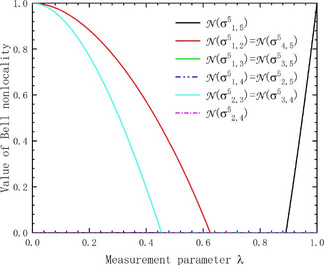
Figure 4. Variations of the value of Bell nonlocality with the measurement parameter λ for the states ${\sigma }_{1,5}^{5}$, ${\sigma }_{1,2}^{5}$, ${\sigma }_{4,5}^{5}$, ${\sigma }_{1,3}^{5}$, ${\sigma }_{3,5}^{5}$, ${\sigma }_{1,4}^{5}$, ${\sigma }_{2,5}^{5}$ ${\sigma }_{2,3}^{5}$, ${\sigma }_{3,4}^{5}$ and ${\sigma }_{2,4}^{5}$. |
4.2. EPR steering
Next, we discuss the quantification of EPR steering of all the post-measurement states in the network of figure 3. From equations (3 ) and (12 ), we get
$\begin{eqnarray*}\begin{array}{l}{ \mathcal S }({\sigma }_{1,5}^{5})=\max \left\{0,\displaystyle \frac{\sqrt{3}{\lambda }^{3}-1}{\sqrt{3}-1}\right\},\\ { \mathcal S }({\sigma }_{1,2}^{5})={ \mathcal S }({\sigma }_{4,5}^{5})=\max \left\{0,\displaystyle \frac{\sqrt{3}s(\lambda )-1}{\sqrt{3}-1}\right\},\end{array}\end{eqnarray*}$
$\begin{eqnarray*}\begin{array}{l}{ \mathcal S }({\sigma }_{1,3}^{5})={ \mathcal S }({\sigma }_{3,5}^{5})=\max \left\{0,\displaystyle \frac{\sqrt{3}\lambda s(\lambda )-1}{\sqrt{3}-1}\right\},\\ { \mathcal S }({\sigma }_{1,4}^{5})={ \mathcal S }({\sigma }_{2,5}^{5})=\max \left\{0,\displaystyle \frac{\sqrt{3}{\lambda }^{2}s(\lambda )-1}{\sqrt{3}-1}\right\},\end{array}\end{eqnarray*}$
$\begin{eqnarray*}\begin{array}{l}{ \mathcal S }({\sigma }_{2,3}^{5})={ \mathcal S }({\sigma }_{3,4}^{5})=\max \left\{0,\displaystyle \frac{\sqrt{3}s{\left(\lambda \right)}^{2}-1}{\sqrt{3}-1}\right\},\\ { \mathcal S }({\sigma }_{2,4}^{5})=\max \left\{0,\displaystyle \frac{\sqrt{3}\lambda s{\left(\lambda \right)}^{2}-1}{\sqrt{3}-1}\right\}.\end{array}\end{eqnarray*}$
Figure 5 gives the EPR steering of all the post-measurement states with the parameter λ. Although figure 5 is similar to figure 4, the EPR steerability of the post-measurement states is in a larger range. Concretely, ${\sigma }_{1,5}^{5}$ is EPR steerable for 0.84 < λ ≤ 1, and is Bell nonlocal for 0.89 < λ ≤ 1; ${\sigma }_{1,2}^{5}$ and ${\sigma }_{4,5}^{5}$ are EPR steerable for 0 ≤ λ < 0.75, and are Bell nonlocal for 0 ≤ λ < 0.62; ${\sigma }_{2,3}^{5}$ and ${\sigma }_{3,4}^{5}$ are EPR steerable for 0 ≤ λ < 0.56, and are Bell nonlocal for 0 ≤ λ < 0.45; and none of the other post-measurement states are EPR steerable.
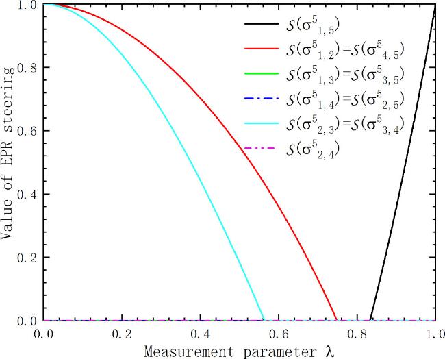
Figure 5. Variations of the value of EPR steering with the measurement parameter λ for the states ${\sigma }_{1,5}^{5}$, ${\sigma }_{1,2}^{5}$ and ${\sigma }_{4,5}^{5}$, ${\sigma }_{1,3}^{5}$ and ${\sigma }_{3,5}^{5}$, ${\sigma }_{1,4}^{5}$ and ${\sigma }_{2,5}^{5}$ ${\sigma }_{2,3}^{5}$ and ${\sigma }_{3,4}^{5}$, ${\sigma }_{2,4}^{5}$. |
4.3. Entanglement
Finally, we analyze the entanglement of all the post-measurement states in the network of figure 3. From direct calculations, we obtain the minimum eigenvalue of ${\left({\sigma }_{\mathrm{1,5}}^{5}\right)}^{{T}_{B}}$ is $\mu ({\left({\sigma }_{\mathrm{1,5}}^{5}\right)}^{{T}_{B}})\,=\tfrac{1-3{\lambda }^{3}}{4}$. Therefore, it follows from equation (4 ) that
$\begin{eqnarray*}{ \mathcal E }({\sigma }_{1,5}^{5})=2\max \left\{0,\displaystyle \frac{3{\lambda }^{3}-1}{4}\right\}.\end{eqnarray*}$
Similarly, both of the minimum eigenvalues of ${\left({\sigma }_{\mathrm{1,2}}^{5}\right)}^{{T}_{B}}$ and ${\left({\sigma }_{\mathrm{4,5}}^{5}\right)}^{{T}_{B}}$ are $\mu ({\left({\sigma }_{\mathrm{1,2}}^{5}\right)}^{{T}_{B}})=\mu ({\left({\sigma }_{\mathrm{4,5}}^{5}\right)}^{{T}_{B}})=\tfrac{1-3s(\lambda )}{4};$ the minimum eigenvalues of ${\left({\sigma }_{\mathrm{1,3}}^{5}\right)}^{{T}_{B}}$ and ${\left({\sigma }_{\mathrm{3,5}}^{5}\right)}^{{T}_{B}}$ are $\mu ({\left({\sigma }_{\mathrm{1,3}}^{5}\right)}^{{T}_{B}})\,=\mu ({\left({\sigma }_{\mathrm{3,5}}^{5}\right)}^{{T}_{B}})=\tfrac{1-3\lambda s(\lambda )}{4};$ the minimum eigenvalues of ${\left({\sigma }_{\mathrm{1,4}}^{5}\right)}^{{T}_{B}}$ and ${\left({\sigma }_{\mathrm{2,5}}^{5}\right)}^{{T}_{B}}$ are $\mu ({\left({\sigma }_{\mathrm{1,4}}^{5}\right)}^{{T}_{B}})=\mu ({\left({\sigma }_{\mathrm{2,5}}^{5}\right)}^{{T}_{B}})=\tfrac{1-3{\lambda }^{2}s(\lambda )}{4};$ the minimum eigenvalues of ${\left({\sigma }_{\mathrm{2,3}}^{5}\right)}^{{T}_{B}}$ and ${\left({\sigma }_{\mathrm{3,4}}^{5}\right)}^{{T}_{B}}$ are $\mu ({\left({\sigma }_{\mathrm{2,3}}^{5}\right)}^{{T}_{B}})\,=\mu ({\left({\sigma }_{\mathrm{3,4}}^{5}\right)}^{{T}_{B}})=\tfrac{1-3s{\left(\lambda \right)}^{2}}{4};$ and the minimum eigenvalue of ${\left({\sigma }_{\mathrm{2,4}}^{5}\right)}^{{T}_{B}}$ is $\mu ({\left({\sigma }_{\mathrm{2,4}}^{5}\right)}^{{T}_{B}})=\tfrac{1-3\lambda s{\left(\lambda \right)}^{2}}{4}$. It follows from equation (4 ) that
$\begin{eqnarray*}\begin{array}{l}{ \mathcal E }({\sigma }_{1,2}^{5})={ \mathcal E }({\sigma }_{4,5}^{5})=2\max \left\{0,\displaystyle \frac{3s(\lambda )-1}{4}\right\},\\ { \mathcal E }({\sigma }_{1,3}^{5})={ \mathcal E }({\sigma }_{3,5}^{5})=2\max \left\{0,\displaystyle \frac{3\lambda s(\lambda )-1}{4}\right\},\end{array}\end{eqnarray*}$
$\begin{eqnarray*}\begin{array}{l}{ \mathcal E }({\sigma }_{1,4}^{5})={ \mathcal E }({\sigma }_{2,5}^{5})=2\max \left\{0,\displaystyle \frac{3{\lambda }^{2}s(\lambda )-1}{4}\right\},\\ { \mathcal E }({\sigma }_{2,3}^{5})={ \mathcal E }({\sigma }_{3,4}^{5})=2\max \left\{0,\displaystyle \frac{3s{\left(\lambda \right)}^{2}-1}{4}\right\},\end{array}\end{eqnarray*}$
and $\begin{eqnarray*}{ \mathcal E }({\sigma }_{2,4}^{5})=2\max \left\{0,\displaystyle \frac{3\lambda s{\left(\lambda \right)}^{2}-1}{4}\right\}.\end{eqnarray*}$
In figure 6, we see that the variations of ${ \mathcal E }({\sigma }_{1,5}^{5})$, ${ \mathcal E }({\sigma }_{1,2}^{5})$, ${ \mathcal E }({\sigma }_{4,5}^{5})$, ${ \mathcal E }({\sigma }_{2,3}^{5})$ and ${ \mathcal E }({\sigma }_{3,4}^{5})$ are similar to those in figures 4 and 5, but the range of λ for entanglement of these post-measurement states is a little wider than the ranges of λ for Bell nonlocality and EPR steerability. When 0.7 < λ ≤ 1, ${\sigma }_{1,5}^{5}$ is entangled; when 0 ≤ λ < 0.91, ${\sigma }_{1,2}^{5}$ and ${\sigma }_{4,5}^{5}$ are entangled; and when 0 ≤ λ < 0.75, ${\sigma }_{2,3}^{5}$ and ${\sigma }_{3,4}^{5}$ are entangled. The big difference between figure 6 and figures 4 and 5 is that when 0.38 < λ < 0.89, ${\sigma }_{1,3}^{5}$ and ${\sigma }_{3,5}^{5}$ are entangled, while ${\sigma }_{1,3}^{5}$, ${\sigma }_{1,4}^{5}$, ${\sigma }_{2,5}^{5}$, ${\sigma }_{2,4}^{5}$, ${\sigma }_{3,4}^{5}$ and ${\sigma }_{3,5}^{5}$ are Bell local or EPR nonsteerable. In addition, there is a small range here that ${\sigma }_{1,5}^{5}$, ${\sigma }_{1,2}^{5}$, ${\sigma }_{4,5}^{5}$, ${\sigma }_{2,3}^{5}$, ${\sigma }_{3,4}^{5}$, ${\sigma }_{1,3}^{5}$ and ${\sigma }_{3,5}^{5}$ are all entangled when 0.7 ≤ λ ≤ 0.75.
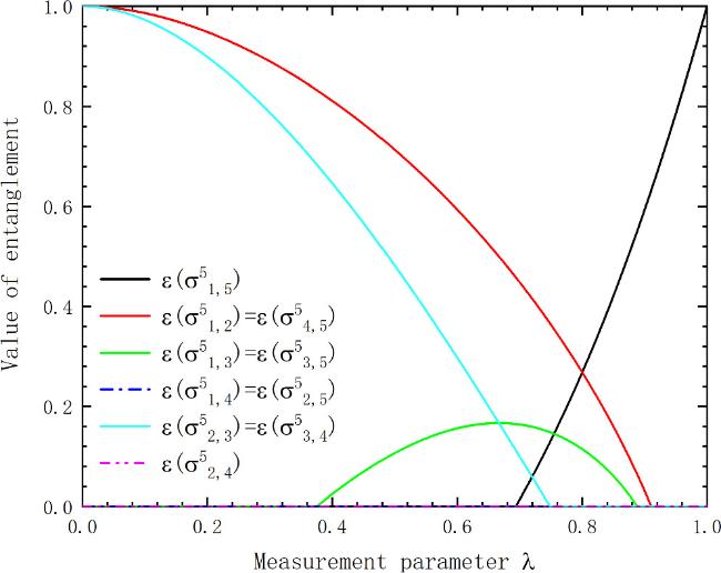
Figure 6. Variations of entanglement with the measurement parameter λ for the states ${\sigma }_{1,5}^{5}$, ${\sigma }_{1,2}^{5}$ and ${\sigma }_{4,5}^{5}$, ${\sigma }_{1,3}^{5}$ and ${\sigma }_{3,5}^{5}$, ${\sigma }_{1,4}^{5}$ and ${\sigma }_{2,5}^{5}$ ${\sigma }_{2,3}^{5}$ and ${\sigma }_{3,4}^{5}$, ${\sigma }_{2,4}^{5}$. |
4.4. The inclusion relation of three quantum correlations
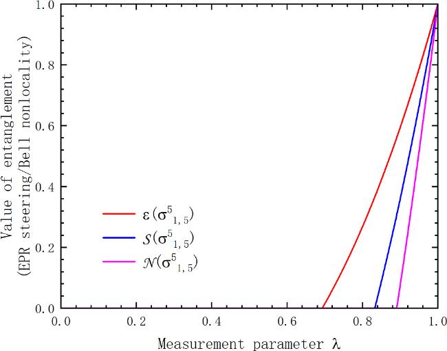
Finally, we analyze in detail the Bell nonlocality, EPR steering and entanglement of some post-measurement states. Take the post-measurement state ${\sigma }_{1,5}^{5}$ for example. In figure 7, we observe that when 0.7 < λ ≤ 1, ${\sigma }_{1,5}^{5}$ is entangled; only if 0.84 < λ ≤ 1, ${\sigma }_{1,5}^{5}$ is EPR steerable; and only if 0.89 < λ ≤ 1, ${\sigma }_{1,5}^{5}$ is Bell nonlocal. From this we can re-verify the inclusion relation of these three quantum correlations: the EPR steerable state is necessarily entangled, while the entanglement state is not necessarily EPR steerable; the Bell nonlocal state is necessarily EPR steerable, while the EPR steerable state is not necessarily Bell nonlocal.
Figure 7. Variations of the value of Bell nonlocality, EPR steering and entanglement with the measurement parameter λ for the state ${\sigma }_{1,5}^{5}$. |
5. Discussion
In the present paper, we consider an n-partite chain network with each of two neighboring observers sharing an arbitrary Bell state and all intermediate observers performing some POVMs with parameter λ, and we discuss the Bell nonlocality, EPR steering and entanglement of all post-measurement states. In particular, for n = 5, we plot the quantification functions of the three quantum correlations with respect to λ, and obtain the range of λ for the post-measurement states that are Bell nonlocal, EPR steerable or entangled. In addition, we find that some post-measurement states exist that do not have three quantum correlations. One may ask which quantum states are uncorrelated, why they are uncorrelated and whether they have other quantum correlations. This is a direction for our future research. Another natural question is how to characterize the general forms of all post-measurement states if the shared state between each two neighboring observers is any quantum state and all intermediate observers perform any POVM measurements.
Appendix
We divide the proof into four cases based on the values of p and q. Write ${\sigma }_{p,q}^{k}={\sigma }_{p,q}^{k}(\vec{{\boldsymbol{u}}};\vec{{\boldsymbol{v}}})$ ($3\leqslant k\leqslant n$) in the sequel.
Case 1. p = 1 and q = n.
In this case, equation (6 ) becomesA1 ) using mathematical induction.
$\begin{eqnarray}{\sigma }_{1,n}^{n}={\lambda }_{2}\cdots {\lambda }_{n-1}| {\psi }_{i}\rangle \langle {\psi }_{i}| +\displaystyle \frac{1-{\lambda }_{2}\cdots {\lambda }_{n-1}}{4}{{\mathbb{I}}}_{4},\end{eqnarray}$
where $\begin{eqnarray}i=\left\{\begin{array}{l}1\ \ \mathrm{if}\ {c}_{3}({\sigma }_{1,n}^{n})+{c}_{4}({\sigma }_{1,n}^{n})\ \mathrm{is}\ \mathrm{even}\ \mathrm{and}\ {c}_{2}({\sigma }_{1,n}^{n})+{c}_{4}({\sigma }_{1,n}^{n})\ \mathrm{is}\ \mathrm{even};\\ 2\ \ \mathrm{if}\ {c}_{3}({\sigma }_{1,n}^{n})+{c}_{4}({\sigma }_{1,n}^{n})\ \mathrm{is}\ \mathrm{even}\ \mathrm{and}\ {c}_{2}({\sigma }_{1,n}^{n})+{c}_{4}({\sigma }_{1,n}^{n})\ \mathrm{is}\ \mathrm{odd};\\ 3\ \ \mathrm{if}\ {c}_{3}({\sigma }_{1,n}^{n})+{c}_{4}({\sigma }_{1,n}^{n})\ \mathrm{is}\ \mathrm{odd}\ \mathrm{and}\ {c}_{2}({\sigma }_{1,n}^{n})+{c}_{4}({\sigma }_{1,n}^{n})\ \mathrm{is}\ \mathrm{even};\\ 4\ \ \mathrm{if}\ {c}_{3}({\sigma }_{1,n}^{n})+{c}_{4}({\sigma }_{1,n}^{n})\ \mathrm{is}\ \mathrm{odd}\ \mathrm{and}\ {c}_{2}({\sigma }_{1,n}^{n})+{c}_{4}({\sigma }_{1,n}^{n})\ \mathrm{is}\ \mathrm{odd}.\\ \end{array}\right.\end{eqnarray}$
We will prove equation (In fact, if n = 3, then equation (A1 ) holds in Remark 1.
Next, assume that equation (A1 ) holds for n = l, i.e. ${\sigma }_{1,l}^{l}={\lambda }_{2}\cdots {\lambda }_{l-1}| {\psi }_{i}\rangle \langle {\psi }_{i}| +\tfrac{1-{\lambda }_{2}\cdots {\lambda }_{l-1}}{4}{{\mathbb{I}}}_{4}$, where
$\begin{eqnarray*}i=\left\{\begin{array}{l}1\ \ \mathrm{if}\ {c}_{3}({\sigma }_{1,l}^{l})+{c}_{4}({\sigma }_{1,l}^{l})\ \mathrm{is}\ \mathrm{even}\ \mathrm{and}\ {c}_{2}({\sigma }_{1,l}^{l})+{c}_{4}({\sigma }_{1,l}^{l})\ \mathrm{is}\ \mathrm{even};\\ 2\ \ \mathrm{if}\ {c}_{3}({\sigma }_{1,l}^{l})+{c}_{4}({\sigma }_{1,l}^{l})\ \mathrm{is}\ \mathrm{even}\ \mathrm{and}\ {c}_{2}({\sigma }_{1,l}^{l})+{c}_{4}({\sigma }_{1,l}^{l})\ \mathrm{is}\ \mathrm{odd};\\ 3\ \ \mathrm{if}\ {c}_{3}({\sigma }_{1,l}^{l})+{c}_{4}({\sigma }_{1,l}^{l})\ \mathrm{is}\ \mathrm{odd}\ \mathrm{and}\ {c}_{2}({\sigma }_{1,l}^{l})+{c}_{4}({\sigma }_{1,l}^{l})\ \mathrm{is}\ \mathrm{even};\\ 4\ \ \mathrm{if}\ {c}_{3}({\sigma }_{1,l}^{l})+{c}_{4}({\sigma }_{1,l}^{l})\ \mathrm{is}\ \mathrm{odd}\ \mathrm{and}\ {c}_{2}({\sigma }_{1,l}^{l})+{c}_{4}({\sigma }_{1,l}^{l})\ \mathrm{is}\ \mathrm{odd}.\\ \end{array}\right.\end{eqnarray*}$
Without loss of generality, let i = 1. Then $\begin{eqnarray}{c}_{3}({\sigma }_{1,l}^{l})+{c}_{4}({\sigma }_{1,l}^{l})\ \ \mathrm{and}\ \ {c}_{2}({\sigma }_{1,l}^{l})+{c}_{4}({\sigma }_{1,l}^{l})\ \ \mathrm{are}\ \mathrm{even}\end{eqnarray}$
and ${\sigma }_{1,l}^{l}={\lambda }_{2}\cdots {\lambda }_{l-1}| {\psi }_{1}\rangle \langle {\psi }_{1}| +\tfrac{1-{\lambda }_{2}\cdots {\lambda }_{l-1}}{4}{{\mathbb{I}}}_{4}$.Now, assume that $n=l+1$, and we will check that equation (A1 ) holds. We first consider the case that ${\rho }_{l,l+1}=| {\psi }_{1}\rangle \langle {\psi }_{1}| $ and ${E}_{1}^{l}={\lambda }_{l}| {\psi }_{1}\rangle \langle {\psi }_{1}| +\tfrac{1-{\lambda }_{l}}{4}{{\mathbb{I}}}_{4}$. Then, from equation (A3 ), it is easy to see that both ${c}_{3}({\sigma }_{1,l+1}^{l+1})+{c}_{4}({\sigma }_{1,l+1}^{l+1})$ and ${c}_{2}({\sigma }_{1,l+1}^{l+1})+{c}_{4}({\sigma }_{1,l+1}^{l+1})$ are even; and
$\begin{eqnarray*}\begin{array}{l}{\sigma }_{1,l+1}^{l+1}=\displaystyle \frac{{\mathrm{Tr}}_{\mathrm{2,2},\cdots ,l,l}[({{\mathbb{P}}}_{2}^{l-1}\otimes \sqrt{{E}_{1}^{l}}\otimes {I}_{l+1})({\rho }_{\mathrm{1,2}}\otimes \cdots \otimes {\rho }_{l,l+1})({\left({{\mathbb{P}}}_{2}^{l-1}\right)}^{\dagger }\otimes {\sqrt{{E}_{1}^{l}}}^{\dagger }\otimes {I}_{l+1})]}{\mathrm{Tr}[({{\mathbb{P}}}_{2}^{l-1}\otimes \sqrt{{E}_{1}^{l}}\otimes {I}_{l+1})({\rho }_{\mathrm{1,2}}\otimes \cdots \otimes {\rho }_{l,l+1})({\left({{\mathbb{P}}}_{2}^{l-1}\right)}^{\dagger }\otimes {\sqrt{{E}_{1}^{l}}}^{\dagger }\otimes {I}_{l+1})]}\\ \quad =\displaystyle \frac{{\mathrm{Tr}}_{l,l}[({I}_{1}\otimes \sqrt{{E}_{1}^{l}}\otimes {I}_{l+1})(({\mathrm{Tr}}_{\mathrm{2,2},\cdots ,l-1,l-1}[({{\mathbb{P}}}_{2}^{l-1})({\rho }_{\mathrm{1,2}}\otimes \cdots \otimes {\rho }_{l-1,l})({\left({{\mathbb{P}}}_{2}^{l-1}\right)}^{\dagger })])\otimes {\rho }_{l,l\,+\,1})({I}_{1}\otimes {\sqrt{{E}_{1}^{l}}}^{\dagger }\otimes {I}_{l+1})]}{\mathrm{Tr}[({I}_{1}\otimes \sqrt{{E}_{1}^{l}}\otimes {I}_{l+1})(({\mathrm{Tr}}_{\mathrm{2,2},\cdots ,l-1,l-1}[({{\mathbb{P}}}_{2}^{l-1})({\rho }_{\mathrm{1,2}}\otimes \cdots \otimes {\rho }_{l-1,l})({\left({{\mathbb{P}}}_{2}^{l-1}\right)}^{\dagger })])\otimes {\rho }_{l,l+1})({I}_{1}\otimes {\sqrt{{E}_{1}^{l}}}^{\dagger }\otimes {I}_{l+1})]}\\ \quad =\displaystyle \frac{{\mathrm{Tr}}_{l,l}[({I}_{1}\otimes \sqrt{{E}_{1}^{l}}\otimes {I}_{l+1})\left(\tfrac{{\mathrm{Tr}}_{\mathrm{2,2},\cdots ,l-1,l-1}[({{\mathbb{P}}}_{2}^{l-1})({\rho }_{\mathrm{1,2}}\otimes \cdots \otimes {\rho }_{l-1,l})({\left({{\mathbb{P}}}_{2}^{l-1}\right)}^{\dagger })]}{\mathrm{Tr}[({{\mathbb{P}}}_{2}^{l-1})({\rho }_{\mathrm{1,2}}\otimes \cdots \otimes {\rho }_{l-1,l})({\left({{\mathbb{P}}}_{2}^{l-1}\right)}^{\dagger })]}\otimes {\rho }_{l,l\,+\,1}\right)({I}_{1}\otimes {\sqrt{{E}_{1}^{l}}}^{\dagger }\otimes {I}_{l+1})]}{\mathrm{Tr}[({I}_{1}\otimes \sqrt{{E}_{1}^{l}}\otimes {I}_{l+1})\left(\tfrac{{\mathrm{Tr}}_{\mathrm{2,2},\cdots ,l-1,l-1}[\left({{\mathbb{P}}}_{2}^{l-1}\right)\left({\rho }_{\mathrm{1,2}}\otimes \cdots \otimes {\rho }_{l-1,l}\right)\left({\left({{\mathbb{P}}}_{2}^{l-1}\right)}^{\dagger }\right)]}{\mathrm{Tr}[({{\mathbb{P}}}_{2}^{l-1})({\rho }_{\mathrm{1,2}}\otimes \cdots \otimes {\rho }_{l-1,l})({\left({{\mathbb{P}}}_{2}^{l-1}\right)}^{\dagger })]}\otimes {\rho }_{l,l+1}\right)({I}_{1}\otimes {\sqrt{{E}_{1}^{l}}}^{\dagger }\otimes {I}_{l+1})]}\\ \quad =\displaystyle \frac{{\mathrm{Tr}}_{l,l}[\left({I}_{1}\otimes \sqrt{{E}_{1}^{l}}\otimes {I}_{l+1}\right)\left({\sigma }_{1,l}^{l}\otimes {\rho }_{l,l+1}\right)\left({I}_{1}\otimes {\sqrt{{E}_{1}^{l}}}^{\dagger }\otimes {I}_{l+1}\right)]}{\mathrm{Tr}[({I}_{1}\otimes \sqrt{{E}_{1}^{l}}\otimes {I}_{l+1})({\sigma }_{1,l}^{l}\otimes {\rho }_{l,l+1})({I}_{1}\otimes {\sqrt{{E}_{1}^{l}}}^{\dagger }\otimes {I}_{l+1})]}.\end{array}\end{eqnarray*}$
Here, ${j}_{2},\cdots ,{j}_{l-1}\in \{1,2,3,4\}$ and ${{\mathbb{P}}}_{2}^{l-1}={I}_{1}{\otimes }_{t=2}^{l-1}\sqrt{{E}_{{j}_{t}}^{t}}$. As $\begin{eqnarray*}\begin{array}{l}\sqrt{{E}_{1}^{l}}={\sqrt{{E}_{1}^{l}}}^{\dagger }=\displaystyle \frac{\left(\sqrt{\tfrac{1+3{\lambda }_{l}}{4}}-\sqrt{\tfrac{1-{\lambda }_{l}}{4}}\right)}{2}\\ \quad \times (| 00\rangle \langle 00| +| 00\rangle \langle 11| +| 11\rangle \langle 00| +| 11\rangle \langle 11| )\\ \quad +\sqrt{\displaystyle \frac{1-{\lambda }_{l}}{4}}(| 00\rangle \langle 00| +| 01\rangle \langle 01| +| 10\rangle \langle 10| +| 11\rangle \langle 11| )\end{array}\end{eqnarray*}$
and $\begin{eqnarray*}\begin{array}{l}{\sigma }_{1,l}^{l}\otimes {\rho }_{l,l+1}=\displaystyle \frac{{\lambda }_{2}\cdots {\lambda }_{l-1}}{4}(| 0000\rangle \langle 0000| \\ \quad +| 0000\rangle \langle 0011| +| 0011\rangle \langle 0000| +| 0011\rangle \langle 0011| \\ \quad +| 0000\rangle \langle 1100| +| 0000\rangle \langle 1111| \\ \quad +| 0011\rangle \langle 1100| +| 0011\rangle \langle 1111| \\ \quad +| 1100\rangle \langle 0000| +| 1100\rangle \langle 0011| \\ \quad +| 1111\rangle \langle 0000| +| 1111\rangle \langle 0011| \\ \quad +| 1100\rangle \langle 1100| +| 1100\rangle \langle 1111| \\ \quad +| 1111\rangle \langle 1100| +| 1111\rangle \langle 1111| )\\ \quad +\displaystyle \frac{1-{\lambda }_{2}\cdots {\lambda }_{l-1}}{8}(| 0000\rangle \langle 0000| +| 0000\rangle \\ \quad \langle 0011| +| 0011\rangle \langle 0000| +| 0011\rangle \langle 0011| \\ \quad +| 0100\rangle \langle 0100| +| 0100\rangle \langle 0111| \\ \quad +| 0111\rangle \langle 0100| +| 0111\rangle \langle 0111| \\ \quad +| 1000\rangle \langle 1000| +| 1000\rangle \langle 1011| \\ \quad +| 1011\rangle \langle 1000| +| 1011\rangle \langle 1011| \\ \quad +| 1100\rangle \langle 1100| +| 1100\rangle \langle 1111| \\ \quad +| 1111\rangle \langle 1100| +| 1111\rangle \langle 1111| ),\end{array}\end{eqnarray*}$
a direct calculation gives $\begin{eqnarray*}\begin{array}{l}\mathrm{Tr}[({I}_{1}\otimes \sqrt{{E}_{1}^{l}}\otimes {I}_{l+1})({\sigma }_{1,l}^{l}\otimes {\rho }_{l,l+1})\\ \quad \times ({I}_{1}\otimes {\sqrt{{E}_{1}^{l}}}^{\dagger }\otimes {I}_{l+1})]=\displaystyle \frac{1}{4},\end{array}\end{eqnarray*}$
and $\begin{eqnarray*}\begin{array}{l}{\mathrm{Tr}}_{l,l}[({I}_{1}\otimes \sqrt{{E}_{1}^{l}}\otimes {I}_{l+1})({\sigma }_{1,l}^{l}\otimes {\rho }_{l,l+1})\\ \quad \times ({I}_{1}\otimes {\sqrt{{E}_{1}^{l}}}^{\dagger }\otimes {I}_{l+1})]=\displaystyle \frac{{\lambda }_{2}\cdots {\lambda }_{l}}{4}| {\psi }_{1}\rangle \langle {\psi }_{1}| \\ \quad +\displaystyle \frac{1-{\lambda }_{2}\cdots {\lambda }_{l}}{16}{{\mathbb{I}}}_{4}.\end{array}\end{eqnarray*}$
So $\begin{eqnarray*}{\sigma }_{1,l+1}^{l+1}={\lambda }_{2}\cdots {\lambda }_{l}| {\psi }_{1}\rangle \langle {\psi }_{1}| +\displaystyle \frac{1-{\lambda }_{2}\cdots {\lambda }_{l}}{4}{{\mathbb{I}}}_{4}.\end{eqnarray*}$
For other cases, using similar arguments to those of the above, one can show that equation (A1 ) still holds.
Case 2. $1=p\lt q\lt n$.
From Case 1, we know that
$\begin{eqnarray*}{\sigma }_{1,q}^{q}={\lambda }_{2}\cdots {\lambda }_{q-1}| {\psi }_{i}\rangle \langle {\psi }_{i}| +\displaystyle \frac{1-{\lambda }_{2}\cdots {\lambda }_{q-1}}{4}{{\mathbb{I}}}_{4},\end{eqnarray*}$
where $\begin{eqnarray*}i=\left\{\begin{array}{l}1\ \ \mathrm{if}\ {c}_{3}({\sigma }_{1,q}^{q})+{c}_{4}({\sigma }_{1,q}^{q})\ \mathrm{is}\ \mathrm{even}\ \mathrm{and}\ {c}_{2}({\sigma }_{1,q}^{q})+{c}_{4}({\sigma }_{1,q}^{q})\ \mathrm{is}\ \mathrm{even};\\ 2\ \ \mathrm{if}\ {c}_{3}({\sigma }_{1,q}^{q})+{c}_{4}({\sigma }_{1,q}^{q})\ \mathrm{is}\ \mathrm{even}\ \mathrm{and}\ {c}_{2}({\sigma }_{1,q}^{q})+{c}_{4}({\sigma }_{1,q}^{q})\ \mathrm{is}\ \mathrm{odd};\\ 3\ \ \mathrm{if}\ {c}_{3}({\sigma }_{1,q}^{q})+{c}_{4}({\sigma }_{1,q}^{q})\ \mathrm{is}\ \mathrm{odd}\ \mathrm{and}\ {c}_{2}({\sigma }_{1,q}^{q})+{c}_{4}({\sigma }_{1,q}^{q})\ \mathrm{is}\ \mathrm{even};\\ 4\ \ \mathrm{if}\ {c}_{3}({\sigma }_{1,q}^{q})+{c}_{4}({\sigma }_{1,q}^{q})\ \mathrm{is}\ \mathrm{odd}\ \mathrm{and}\ {c}_{2}({\sigma }_{1,q}^{q})+{c}_{4}({\sigma }_{1,q}^{q})\ \mathrm{is}\ \mathrm{odd}.\end{array}\right.\end{eqnarray*}$
So $\begin{eqnarray}\begin{array}{l}{\sigma }_{1,q}^{q+1}=\displaystyle \frac{{\mathrm{Tr}}_{\mathrm{1,2,2},\cdots ,q-1,q-1,q+1}[\left({I}_{1}{\otimes }_{t=2}^{q}\sqrt{{E}_{{j}_{t}}^{t}}\otimes {I}_{q+1}\right)\left({\rho }_{\mathrm{1,2}}\otimes \cdots \otimes {\rho }_{q,q+1}\right)\left({I}_{1}{\otimes }_{t=2}^{q}{\sqrt{{E}_{{j}_{t}}^{t}}}^{\dagger }\otimes {I}_{q+1}\right)]}{\mathrm{Tr}[({I}_{1}{\otimes }_{t=2}^{q}\sqrt{{E}_{{j}_{t}}^{t}}\otimes {I}_{q+1})({\rho }_{\mathrm{1,2}}\otimes \cdots \otimes {\rho }_{q,q+1})({I}_{1}{\otimes }_{t=2}^{q}{\sqrt{{E}_{{j}_{t}}^{t}}}^{\dagger }\otimes {I}_{q+1})]}\\ \quad =\displaystyle \frac{{\mathrm{Tr}}_{q,q+1}[({I}_{1}\otimes \sqrt{{E}_{{j}_{q}}^{q}}\otimes {I}_{q+1})({\sigma }_{1,q}^{q}\otimes {\rho }_{q,q+1})({I}_{1}\otimes {\sqrt{{E}_{{j}_{q}}^{q}}}^{\dagger }\otimes {I}_{q+1})]}{\mathrm{Tr}[({I}_{1}\otimes \sqrt{{E}_{{j}_{q}}^{q}}\otimes {I}_{q+1})({\sigma }_{1,q}^{q}\otimes {\rho }_{q,q+1})({I}_{1}\otimes {\sqrt{{E}_{{j}_{q}}^{q}}}^{\dagger }\otimes {I}_{q+1})]},\end{array}\end{eqnarray}$
where ${j}_{2},\cdots ,{j}_{q}\in \{1,2,3,4\}$. Similar to the proof from ${\sigma }_{1,l}^{l}$ to ${\sigma }_{1,l+1}^{l+1}$ in Case 1, one can get $\begin{eqnarray*}{\sigma }_{1,q}^{q+1}={\lambda }_{2}\cdots {\lambda }_{q-1}s({\lambda }_{q})| {\psi }_{i}\rangle \langle {\psi }_{i}| +\displaystyle \frac{1-{\lambda }_{2}\cdots {\lambda }_{q-1}s({\lambda }_{q})}{4}{{\mathbb{I}}}_{4},\end{eqnarray*}$
where $\begin{eqnarray*}i=\left\{\begin{array}{l}1\ \ \mathrm{if}\ {c}_{3}({\sigma }_{1,q}^{q+1})+{c}_{4}({\sigma }_{1,q}^{q+1})\ \mathrm{is}\ \mathrm{even}\ \mathrm{and}\ {c}_{2}({\sigma }_{1,q}^{q+1})+{c}_{4}({\sigma }_{1,q}^{q+1})\ \mathrm{is}\ \mathrm{even};\\ 2\ \ \mathrm{if}\ {c}_{3}({\sigma }_{1,q}^{q+1})+{c}_{4}({\sigma }_{1,q}^{q+1})\ \mathrm{is}\ \mathrm{even}\ \mathrm{and}\ {c}_{2}({\sigma }_{1,q}^{q+1})+{c}_{4}({\sigma }_{1,q}^{q+1})\ \mathrm{is}\ \mathrm{odd};\\ 3\ \ \mathrm{if}\ {c}_{3}({\sigma }_{1,q}^{q+1})+{c}_{4}({\sigma }_{1,q}^{q+1})\ \mathrm{is}\ \mathrm{odd}\ \mathrm{and}\ {c}_{2}({\sigma }_{1,q}^{q+1})+{c}_{4}({\sigma }_{1,q}^{q+1})\ \mathrm{is}\ \mathrm{even};\\ 4\ \ \mathrm{if}\ {c}_{3}({\sigma }_{1,q}^{q+1})+{c}_{4}({\sigma }_{1,q}^{q+1})\ \mathrm{is}\ \mathrm{odd}\ \mathrm{and}\ {c}_{2}({\sigma }_{1,q}^{q+1})+{c}_{4}({\sigma }_{1,q}^{q+1})\ \mathrm{is}\ \mathrm{odd}.\end{array}\right.\end{eqnarray*}$
Next, we claimA2 ), completing the proof of the case.
$\begin{eqnarray}{\sigma }_{1,q}^{q+k}={\sigma }_{1,q}^{q+1}\ \ \mathrm{for}\ \mathrm{any}\ \mathrm{integer}\ \ k\geqslant 2\ \ \mathrm{with}\ \ q+k\leqslant n,\end{eqnarray}$
and so $\begin{eqnarray*}{\sigma }_{1,q}^{n}={\lambda }_{2}\cdots {\lambda }_{q-1}s({\lambda }_{q})| {\psi }_{i}\rangle \langle {\psi }_{i}| +\displaystyle \frac{1-{\lambda }_{2}\cdots {\lambda }_{q-1}s({\lambda }_{q})}{4}{{\mathbb{I}}}_{4},\end{eqnarray*}$
where i takes the values in equation (To do this, take any orthonormal bases $\{{u}_{1},{u}_{2}\}$ of ${H}_{q,1}$ and $\{{v}_{1},{v}_{2}\}$ of ${H}_{q,2}$, and write ${U}_{{ij}}={u}_{i}\otimes {u}_{j}$ and ${V}_{{ij}}={v}_{i}\otimes {v}_{j}$. Then $\sqrt{{E}_{{j}_{q}}^{q}}$ can be written as
$\begin{eqnarray*}\begin{array}{l}\sqrt{{E}_{{j}_{q}}^{q}}=\displaystyle \sum _{i,j=1;k,l=1}{t}_{{ij},{kl}}{U}_{{ij}}\otimes {V}_{{kl}}\\ \quad =\displaystyle \sum _{i,j=1}{U}_{{ij}}\otimes \displaystyle \sum _{k,l=1}{t}_{{ij},{kl}}{V}_{{kl}}.\end{array}\end{eqnarray*}$
Let ${\mathbb{U}}={\sum }_{i,j=1}{U}_{{ij}}$, ${\mathbb{V}}={\sum }_{k,l=1}{t}_{{ij},{kl}}{V}_{{kl}}$, ${{\mathbb{P}}}_{2}^{q+k-1}={I}_{1}{\otimes }_{t=2}^{q+k-1}\sqrt{{E}_{{j}_{t}}^{t}}$, ${{\mathbb{P}}}_{2}^{q-1}={I}_{1}{\otimes }_{t=2}^{q-1}\sqrt{{E}_{{j}_{t}}^{t}},$ ${{\mathbb{P}}}_{q+1}^{q+k-1}={\otimes }_{t=q+1}^{q+k-1}\sqrt{{E}_{{j}_{t}}^{t}}\otimes {I}_{q+k}$ and ${{\mathbb{P}}}_{2}^{q}={I}_{1}{\otimes }_{t=2}^{q}\sqrt{{E}_{{j}_{t}}^{t}}$. Then $\begin{eqnarray*}\begin{array}{l}{\sigma }_{1,q}^{q+k}=\displaystyle \frac{{\mathrm{Tr}}_{\mathrm{2,2},\cdots ,q-1,q-1,q,q+1,q+1,\cdots ,q+k}[({{\mathbb{P}}}_{2}^{q+k-1}\otimes {I}_{q+k})({\rho }_{\mathrm{1,2}}\otimes \cdots \otimes {\rho }_{q+k-1,q+k})({\left({{\mathbb{P}}}_{2}^{q+k-1}\right)}^{\dagger }\otimes {I}_{q+k})]}{\mathrm{Tr}[({{\mathbb{P}}}_{2}^{q+k-1}\otimes {I}_{q+k})({\rho }_{\mathrm{1,2}}\otimes \cdots \otimes {\rho }_{q+k-1,q+k})({\left({{\mathbb{P}}}_{2}^{q+k-1}\right)}^{\dagger }\otimes {I}_{q+k})]}\\ \quad =\displaystyle \frac{{\mathrm{Tr}}_{\mathrm{2,2},\cdots ,q-1,q-1,q,q\,+\,1,q\,+\,1,\cdots ,q\,+\,k}[({{\mathbb{P}}}_{2}^{q-1}\otimes {\mathbb{U}}\otimes {\mathbb{V}}\otimes {{\mathbb{P}}}_{q+1}^{q+k-1})({\rho }_{\mathrm{1,2}}\otimes \cdots \otimes {\rho }_{q+k-1,q+k})({\left({{\mathbb{P}}}_{2}^{q-1}\right)}^{\dagger }\otimes {\mathbb{U}}\otimes {\mathbb{V}}\otimes {\left({{\mathbb{P}}}_{q+1}^{q+k-1}\right)}^{\dagger })]}{\mathrm{Tr}[({{\mathbb{P}}}_{2}^{q-1}\otimes {\mathbb{U}}\otimes {\mathbb{V}}\otimes {{\mathbb{P}}}_{q+1}^{q+k-1})({\rho }_{\mathrm{1,2}}\otimes \cdots \otimes {\rho }_{q+k-1,q+k})({\left({{\mathbb{P}}}_{2}^{q-1}\right)}^{\dagger }\otimes {\mathbb{U}}\otimes {\mathbb{V}}\otimes {\left({{\mathbb{P}}}_{q+1}^{q+k-1}\right)}^{\dagger })]}\\ \quad =\displaystyle \frac{{\mathrm{Tr}}_{\mathrm{2,2},\cdots ,q-1,q-1}[\left({{\mathbb{P}}}_{2}^{q-1}\otimes {\mathbb{U}}\right)\left({\rho }_{\mathrm{1,2}}\otimes \cdots \otimes {\rho }_{q-1,q}\right)\left({\left({{\mathbb{P}}}_{2}^{q-1}\right)}^{\dagger }\otimes {\mathbb{U}}\right)]}{{\mathrm{Tr}}_{\mathrm{1,2,2},\cdots ,q-1,q-1,q}[({P}_{2}^{q-1}\otimes {\mathbb{U}})({\rho }_{\mathrm{1,2}}\otimes \cdots \otimes {\rho }_{q-1,q})({\left({{\mathbb{P}}}_{2}^{q-1}\right)}^{\dagger }\otimes {\mathbb{U}})]}\\ \quad \cdot \displaystyle \frac{{\mathrm{Tr}}_{q,q\,+\,1,q\,+\,1,\cdots ,q\,+\,k}[({\mathbb{V}}\otimes {{\mathbb{P}}}_{q+1}^{q+k-1})({\rho }_{q,q+1}\otimes \cdots \otimes {\rho }_{q+k-1,q+k})({\mathbb{V}}\otimes {\left({{\mathbb{P}}}_{q+1}^{q+k-1}\right)}^{\dagger })]}{{\mathrm{Tr}}_{q,q\,+\,1,q\,+\,1,\cdots ,q\,+\,k}[({\mathbb{V}}\otimes {{\mathbb{P}}}_{q+1}^{q+k-1})({\rho }_{q,q+1}\otimes \cdots \otimes {\rho }_{q+k-1,q+k})({\mathbb{V}}\otimes {\left({{\mathbb{P}}}_{q+1}^{q+k-1}\right)}^{\dagger })]}\\ \quad =\displaystyle \frac{{\mathrm{Tr}}_{\mathrm{2,2},\cdots ,q-1,q-1}[\left({{\mathbb{P}}}_{2}^{q-1}\otimes {\mathbb{U}}\right)\left({\rho }_{\mathrm{1,2}}\otimes \cdots \otimes {\rho }_{q-1,q}\right)\left({\left({{\mathbb{P}}}_{2}^{q-1}\right)}^{\dagger }\otimes {\mathbb{U}}\right)]}{{\mathrm{Tr}}_{\mathrm{1,2,2},\cdots ,q-1,q-1,q}[({{\mathbb{P}}}_{2}^{q-1}\otimes {\mathbb{U}})({\rho }_{\mathrm{1,2}}\otimes \cdots \otimes {\rho }_{q-1,q})({\left({{\mathbb{P}}}_{2}^{q-1}\right)}^{\dagger }\otimes {\mathbb{U}})]},\end{array}\end{eqnarray*}$
and $\begin{eqnarray*}\begin{array}{l}{\sigma }_{1,q}^{q+1}=\displaystyle \frac{{\mathrm{Tr}}_{\mathrm{2,2},\cdots ,q-1,q-1,q,q+1}[({{\mathbb{P}}}_{2}^{q}\otimes {I}_{q+1})({\rho }_{\mathrm{1,2}}\otimes \cdots \otimes {\rho }_{q-1,q}\otimes {\rho }_{q,q+1})({\left({{\mathbb{P}}}_{2}^{q}\right)}^{\dagger }\otimes {I}_{q+1})]}{\mathrm{Tr}[({{\mathbb{P}}}_{2}^{q}\otimes {I}_{q+1})({\rho }_{\mathrm{1,2}}\otimes \cdots \otimes {\rho }_{q-1,q}\otimes {\rho }_{q,q+1})({\left({{\mathbb{P}}}_{2}^{q}\right)}^{\dagger }\otimes {I}_{q+1})]}\\ \quad =\displaystyle \frac{{\mathrm{Tr}}_{\mathrm{2,2},\cdots ,q-1,q-1,q,q\,+\,1}[({{\mathbb{P}}}_{2}^{q-1}\otimes {\mathbb{U}}\otimes {\mathbb{V}}\otimes {I}_{q+1})({\rho }_{\mathrm{1,2}}\otimes \cdots \otimes {\rho }_{q-1,q}\otimes {\rho }_{q,q+1})({\left({{\mathbb{P}}}_{2}^{q-1}\right)}^{\dagger }\otimes {\mathbb{U}}\otimes {\mathbb{V}}\otimes {I}_{q+1})]}{\mathrm{Tr}[({{\mathbb{P}}}_{2}^{q-1}\otimes {\mathbb{U}}\otimes {\mathbb{V}}\otimes {I}_{q+1})({\rho }_{\mathrm{1,2}}\otimes \cdots \otimes {\rho }_{q-1,q}\otimes {\rho }_{q,q+1})({\left({{\mathbb{P}}}_{2}^{q-1}\right)}^{\dagger }\otimes {\mathbb{U}}\otimes {\mathbb{V}}\otimes {I}_{q+1})]}\\ \quad =\displaystyle \frac{{\mathrm{Tr}}_{\mathrm{2,2},\cdots ,q-1,q-1}\left[\left({{\mathbb{P}}}_{2}^{q-1}\otimes {\mathbb{U}}\right)\left({\rho }_{\mathrm{1,2}}\otimes \cdots \otimes {\rho }_{q-1,q}\right)\left({\left({{\mathbb{P}}}_{2}^{q-1}\right)}^{\dagger }\otimes {\mathbb{U}}\right)\right]\cdot {\mathrm{Tr}}_{q,q\,+\,1}[\left({\mathbb{V}}\otimes {I}_{q+1}\right){\rho }_{q,q+1}\left({\mathbb{V}}\otimes {I}_{q+1}\right)]}{{\mathrm{Tr}}_{\mathrm{1,2,2},\cdots ,q-1,q-1,q}[({{\mathbb{P}}}_{2}^{q-1}\otimes {\mathbb{U}})({\rho }_{\mathrm{1,2}}\otimes \cdots \otimes {\rho }_{q-1,q})({\left({{\mathbb{P}}}_{2}^{q-1}\right)}^{\dagger }\otimes {\mathbb{U}})]\cdot {\mathrm{Tr}}_{q,q\,+\,1}[({\mathbb{V}}\otimes {I}_{q+1}){\rho }_{q,q+1}({\mathbb{V}}\otimes {I}_{q+1})]}\\ \quad =\displaystyle \frac{{\mathrm{Tr}}_{\mathrm{2,2},\cdots ,q-1,q-1}[\left({{\mathbb{P}}}_{2}^{q-1}\otimes {\mathbb{U}}\right)\left({\rho }_{\mathrm{1,2}}\otimes \cdots \otimes {\rho }_{q-1,q}\right)\left({\left({{\mathbb{P}}}_{2}^{q-1}\right)}^{\dagger }\otimes {\mathbb{U}}\right)]}{{\mathrm{Tr}}_{\mathrm{1,2,2},\cdots ,q-1,q-1,q}[({{\mathbb{P}}}_{2}^{q-1}\otimes {\mathbb{U}})({\rho }_{\mathrm{1,2}}\otimes \cdots \otimes {\rho }_{q-1,q})({\left({{\mathbb{P}}}_{2}^{q-1}\right)}^{\dagger }\otimes {\mathbb{U}})]},\end{array}\end{eqnarray*}$
which implies ${\sigma }_{1,q}^{q+k}={\sigma }_{1,q}^{q+1}$.Case 3. $1\lt p\lt q=n$.
The proof is similar to that of Case 2 and we omit it here.
Case 4. $1\lt p\lt q\lt n$.
From Case 3, we haveA4 ) and (A5 ), one can show thatA2 ).
$\begin{eqnarray*}\begin{array}{l}{\sigma }_{p,q}^{q}=s({\lambda }_{p}){\lambda }_{p+1}\cdots {\lambda }_{q-1}| {\psi }_{i}\rangle \langle {\psi }_{i}| \\ \,+\displaystyle \frac{1-s\left({\lambda }_{p}\right){\lambda }_{p+1}\cdots {\lambda }_{q-1}}{4}{\mathbb{I}},\end{array}\end{eqnarray*}$
where $\begin{eqnarray*}i=\left\{\begin{array}{l}1\ \ \mathrm{if}\ {c}_{3}({\sigma }_{p,q}^{q})+{c}_{4}({\sigma }_{p,q}^{q})\ \mathrm{is}\ \mathrm{even}\ \mathrm{and}\ {c}_{2}({\sigma }_{p,q}^{q})+{c}_{4}({\sigma }_{p,q}^{q})\ \mathrm{is}\ \mathrm{even};\\ 2\ \ \mathrm{if}\ {c}_{3}({\sigma }_{p,q}^{q})+{c}_{4}({\sigma }_{p,q}^{q})\ \mathrm{is}\ \mathrm{even}\ \mathrm{and}\ {c}_{2}({\sigma }_{p,q}^{q})+{c}_{4}({\sigma }_{p,q}^{q})\ \mathrm{is}\ \mathrm{odd};\\ 3\ \ \mathrm{if}\ {c}_{3}({\sigma }_{p,q}^{q})+{c}_{4}({\sigma }_{p,q}^{q})\ \mathrm{is}\ \mathrm{odd}\ \mathrm{and}\ {c}_{2}({\sigma }_{p,q}^{q})+{c}_{4}({\sigma }_{p,q}^{q})\ \mathrm{is}\ \mathrm{even};\\ 4\ \ \mathrm{if}\ {c}_{3}({\sigma }_{p,q}^{q})+{c}_{4}({\sigma }_{p,q}^{q})\ \mathrm{is}\ \mathrm{odd}\ \mathrm{and}\ {c}_{2}({\sigma }_{p,q}^{q})+{c}_{4}({\sigma }_{p,q}^{q})\ \mathrm{is}\ \mathrm{odd}.\end{array}\right.\end{eqnarray*}$
Now, from similar arguments to those of equations ( $\begin{eqnarray*}{\sigma }_{p,q}^{q+1}=s({\lambda }_{p}){\lambda }_{p+1}\cdots {\lambda }_{q-1}s({\lambda }_{q})| {\psi }_{i}\rangle \langle {\psi }_{i}| +\displaystyle \frac{1-s\left({\lambda }_{p}\right){\lambda }_{p+1}\cdots {\lambda }_{q-1}s({\lambda }_{q})}{4}{{\mathbb{I}}}_{4},\end{eqnarray*}$
and $\begin{eqnarray*}\begin{array}{l}{\sigma }_{p,q}^{n}={\sigma }_{p,q}^{q+1}=s({\lambda }_{p}){\lambda }_{p+1}\cdots {\lambda }_{q-1}s({\lambda }_{q})| {\psi }_{i}\rangle \langle {\psi }_{i}| \\ \quad +\displaystyle \frac{1-s\left({\lambda }_{p}\right){\lambda }_{p+1}\cdots {\lambda }_{q-1}s({\lambda }_{q})}{4}{{\mathbb{I}}}_{4},\end{array}\end{eqnarray*}$
where the values of i are taken by equation (