


1. Introduction
2. A brief review on the Bardeen–Kiselev BH with the cosmological constant
3. Gravitational and electromagnetic perturbations
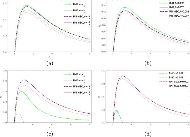
Figure 1. (a) The effective potential V(r) for the Bardeen–Kiselev BH with the cosmological constant and the RN-dSQ for M = 1, c = 0.01 q = 0.1, l = 2 and λ = 0.002 in gravitational perturbations; (b) the effective potential V(r) for the Bardeen–Kiselev BH with the cosmological constant and the RN-dSQ for M = 1, c = 0.01 q = 0.2, l = 2 and w = −2/3 in gravitational perturbations; (c) the effective potential V(r) for the Bardeen–Kiselev BH with the cosmological constant and the RN-dSQ for M = 1, c = 0.01 q = 0.1, l = 2 and λ = 0.002 in electromagnetic perturbations; (d) the effective potential V(r) for the Bardeen–Kiselev BH with the cosmological constant and the RN-dSQ for M = 1, c = 0.01 q = 0.1, l = 2 and w = −2/3 in electromagnetic perturbations. |
4. The QNMs of the Bardeen–Kiselev BH with the cosmological constant for gravitational and electromagnetic perturbations
| 1. | 1. Pure ingoing waves at the event horizon ${\rm{\Psi }}(r)\sim {{\rm{e}}}^{-{\rm{i}}\omega {r}_{* }}$, r* → − ∞ (r → r+), |
| 2. | 2. Pure outgoing waves at the spatial infinity ${\rm{\Psi }}(r)\sim {{\rm{e}}}^{{\rm{i}}\omega {r}_{* }}$, r* → ∞ (r → rc). |
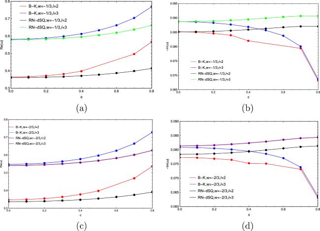
Figure 2. (a) Variation of Re ω with the magnetic charge q for the state parameter w = −1/3; (b) Variation of -Im ω with the magnetic charge q for the state parameter w = −1/3; (c) Variation of Re ω with the magnetic charge q for the state parameter w = −2/3; (d) Variation of -Im ω with the magnetic charge q for the state parameter w = −2/3. In both cases, we take M = 1, c = 0.01 and λ = 0.001. |
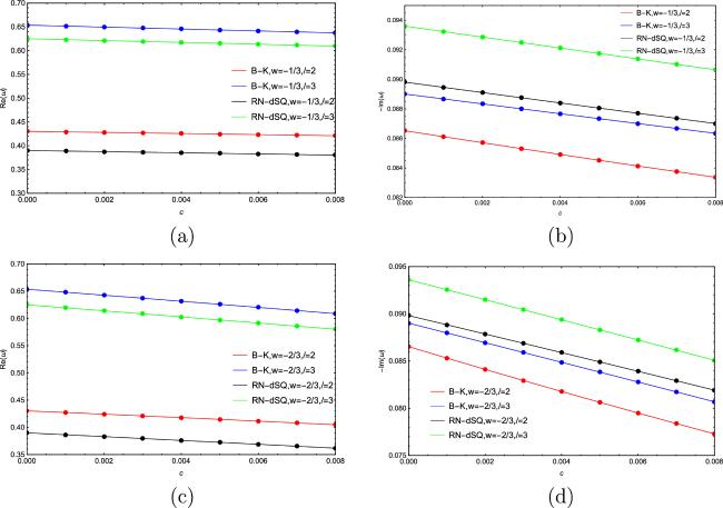
Figure 3. (a) Variation of Re ω with the normalization factor c for the state parameter w = −1/3; (b) Variation of -Im ω with the normalization factor c for the state parameter w = −1/3; (c) Variation of Re ω with the normalization factor c for the state parameter w = −2/3; (d) Variation of -Im ω with the normalization factor c for the state parameter w = −2/3. In both cases, we take M = 1, q = 0.5 and λ = 0.001. |
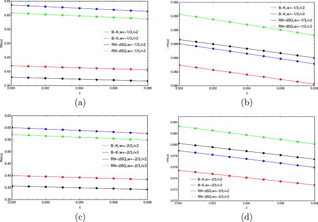
Figure 4. (a) Variation of Re ω with the cosmological constant λ for the state parameter w = −1/3; (b) Variation of -Im ω with the cosmological constant λ for the state parameter w = −1/3; (c) Variation of Re ω with the cosmological constant λ for the state parameter w = −2/3; (d) Variation of -Im ω with the cosmological constant λ for the state parameter w = −2/3. In both cases, we take M = 1, q = 0.5 and c = 0.01. |
Table 1. QNM frequencies of electromagnetic field perturbation for the Bardeen–Kiselev BH with the cosmological constant and the RN-dSQ. |
| M = 1, c = 0.01, λ = 0.001, w = −1/3 | ||||
|---|---|---|---|---|
| ℓ = 2 | ℓ = 3 | |||
| | ||||
| RN-dSQ | Bardeen–Kiselev | RN-dSQ | Bardeen–Kiselev | |
| | ||||
| q = 0.1 | 0.442 872-0.0908932 i | 0.367 24-0.119367 i | 0.635 522-0.0914572 i | 0.535 244-0.121049 i |
| q = 0.2 | 0.445 194-0.0910523 i | 0.495 555-0.112316 i | 0.638 784-0.0916127 i | 0.693 571-0.110998 i |
| q = 0.3 | 0.449 182-0.0913118 i | 0.539 53-0.104102 i | 0.644 385-0.0918663 i | 0.744 857-0.10253 i |
| q = 0.4 | 0.455 032-0.0916603 i | 0.557 533-0.0977495 i | 0.652 595-0.092206 i | 0.764 12-0.0965164 i |
| q = 0.5 | 0.463 062-0.0920738 i | 0.564 534-0.0929304 i | 0.663 858-0.0926075 i | 0.770 024-0.0921494 i |
| q = 0.6 | 0.473 784-0.0925008 i | 0.565 716-0.089275 i | 0.678 878-0.0930191 i | 0.771 675-0.0888982 i |
| | ||||
| M = 1, c = 0.01, λ = 0.001, w = −2/3 | ||||
| | ||||
| ℓ = 2 | ℓ = 3 | |||
| | ||||
| RN-dSQ | Bardeen–Kiselev | RN-dSQ | Bardeen–Kiselev | |
| | ||||
| q = 0.1 | 0.414 383-0.0831505 i | 0.198 681-0.152195 i | 0.594 251-0.0836431 i | 0.306 161-0.14864 i |
| q = 0.2 | 0.416 746-0.0833475 i | 0.369 186-0.129174 i | 0.597 58-0.0838376 i | 0.532 669-0.126129 i |
| q = 0.3 | 0.420 804-0.0836725 i | 0.437 717-0.118541 i | 0.603 296-0.0841582 i | 0.619 425-0.115049 i |
| q = 0.4 | 0.426 758-0.0841178 i | 0.471 818-0.110363 i | 0.611 676-0.084597 i | 0.660 201-0.10686 i |
| q = 0.5 | 0.434 935-0.0846656 i | 0.489 898-0.103874 i | 0.623 176-0.0851359 i | 0.680 26-0.100461 i |
| q = 0.6 | 0.445 858-0.0852751 i | 0.498 972-0.0987989 i | 0.638521-0.0857336 i | 0.688 793-0.0954421 i |
| q = 0.7 | 0.460 387-0.0858485 i | 0.502 352-0.0949737 i | 0.658901-0.0862925 i | 0.689 691-0.091777 i |
Table 2. QNM frequencies of electromagnetic field perturbation for the Bardeen–Kiselev BH with the cosmological constant and the RN-dSQ. |
| M = 1, q = 0.5, λ = 0.001, w = −1/3 | ||||
|---|---|---|---|---|
| ℓ = 2 | ℓ = 3 | |||
| | ||||
| RN-dSQ | Bardeen–Kiselev | RN-dSQ | Bardeen–Kiselev | |
| | ||||
| c = 0 | 0.477 653-0.0958952 i | 0.606 26-0.0854858 i | 0.684 955-0.0964615 i | 0.821 065-0.0871122 i |
| c = 0.001 | 0.476 187-0.0955096 i | 0.602 076-0.086518 i | 0.682 835-0.0960726 i | 0.815 86-0.0878153 i |
| c = 0.002 | 0.474 722-0.0951248 i | 0.597 886-0.0874856 i | 0.680717-0.0956845 i | 0.810 674-0.0884689 i |
| c = 0.003 | 0.473 259-0.0947407 i | 0.593 691-0.0883888 i | 0.678 601-0.0952971 i | 0.805 508-0.0890751 i |
| c = 0.004 | 0.471 798-0.0943574 i | 0.589 495-0.0892268 i | 0.676 488-0.0949106 i | 0.800 365-0.0896358 i |
| c = 0.005 | 0.470338-0.0939749 i | 0.585 301-0.0899992 i | 0.674 377-0.0945248 i | 0.795 244-0.0901527 i |
| c = 0.006 | 0.468 88-0.0935932 i | 0.581 113-0.0907068 i | 0.672 268-0.0941398 i | 0.790 147-0.0906279 i |
| c = 0.007 | 0.467 423-0.0932122 i | 0.576 938-0.0913509 i | 0.670 162-0.0937555 i | 0.785 076-0.0910633 i |
| c = 0.008 | 0.465 968-0.0928319 i | 0.572 78-0.0919342 i | 0.668 058-0.0933721 i | 0.780 031-0.0914606 i |
| | ||||
| M = 1, q = 0.5, λ = 0.001, w = −2/3 | ||||
| | ||||
| ℓ = 2 | ℓ = 3 | |||
| | ||||
| RN-dSQ | Bardeen–Kiselev | RN-dSQ | Bardeen–Kiselev | |
| | ||||
| c = 0 | 0.477 653-0.0958952 i | 0.606 26-0.0854858 i | 0.684 955-0.0964615 i | 0.821 065-0.0871122 i |
| c = 0.001 | 0.473 505-0.0947854 i | 0.595 604-0.0916735 i | 0.678 952-0.095342 i | 0.806 694-0.0909355 i |
| c = 0.002 | 0.469 331-0.0936729 i | 0.582 242-0.0972697 i | 0.672 913-0.0942198 i | 0.791 951-0.0941978 i |
| c = 0.003 | 0.465 131-0.0925576 i | 0.568 667-0.100549 i | 0.666 837-0.0930948i | 0.777 026-0.0966223 i |
| c = 0.004 | 0.460 904-0.0914394i | 0.556 067-0.102324 i | 0.660 722-0.091967 i | 0.762 317-0.0982896 i |
| c = 0.005 | 0.456 649-0.0903182i | 0.544 186-0.103322 i | 0.654 568-0.0908362 i | 0.747 943-0.0993956 i |
| c = 0.006 | 0.452 366-0.089194i | 0.532 764-0.103887 i | 0.648 375-0.0897024 i | 0.733 896-0.100096 i |
| c = 0.007 | 0.448 054-0.0880668 i | 0.521 673-0.104168 i | 0.642 14-0.0885656 i | 0.720 137-0.100496 i |
| c = 0.008 | 0.443 712-0.0869363 i | 0.510 851-0.104236 i | 0.635 862-0.0874256 i | 0.706 63-0.100662 i |
Table 3. QNM frequencies of electromagnetic field perturbation for the Bardeen–Kiselev BH with the cosmological constant and the RN-dSQ. |
| M = 1, q = 0.5, c = 0.01, w = −1/3 | ||||
|---|---|---|---|---|
| ℓ = 2 | ℓ = 3 | |||
| | ||||
| RN-dSQ | Bardeen–Kiselev | RN-dSQ | Bardeen–Kiselev | |
| | ||||
| λ = 0 | 0.465 071-0.0924752 i | 0.567 498-0.0933613 i | 0.666 761-0.0930134 i | 0.773 717-0.0925742 i |
| λ = 0.001 | 0.463 062-0.0920738 i | 0.564 534-0.0929304 i | 0.663 858-0.0926075 i | 0.770 024-0.0921494 i |
| λ = 0.002 | 0.461 044-0.0916706 i | 0.561 566-0.0924977 i | 0.660 941-0.0921997 i | 0.766 32-0.0917227 i |
| λ = 0.003 | 0.459 016-0.0912657 i | 0.558 593-0.0920629 i | 0.658 011-0.0917902 i | 0.762 605-0.0912941 i |
| λ = 0.004 | 0.456 979-0.0908589 i | 0.555 615-0.0916263 i | 0.655 067-0.0913788 i | 0.758 877-0.0908635 i |
| λ = 0.005 | 0.454 931-0.0904504 i | 0.552 631-0.0911876 i | 0.652 11-0.0909656 i | 0.755 138-0.090431 i |
| λ = 0.006 | 0.452 875-0.09004 i | 0.549 642-0.0907469 i | 0.649 139-0.0905504 i | 0.751 386-0.0899965 i |
| λ = 0.007 | 0.450808-0.0896277 i | 0.546 647-0.0903042 i | 0.646 154-0.0901334 i | 0.747 622-0.08956 i |
| λ = 0.008 | 0.448 731-0.0892135 i | 0.543 646-0.0898594 i | 0.643 155-0.0897144 i | 0.743 845-0.0891215 i |
| | ||||
| M = 1, q = 0.5, c = 0.01, w = −2/3 | ||||
| | ||||
| ℓ = 2 | ℓ = 3 | |||
| | ||||
| RN-dSQ | Bardeen–Kiselev | RN-dSQ | Bardeen–Kiselev | |
| | ||||
| λ = 0 | 0.437 079-0.085085 i | 0.492 648-0.104614 i | 0.626 273-0.0855598 i | 0.683 868-0.101142 i |
| λ = 0.001 | 0.434 935-0.0846656 i | 0.489 898-0.103874 i | 0.623 176-0.0851359 i | 0.680 26-0.100461 i |
| λ = 0.002 | 0.432 779-0.0842442 i | 0.487 139-0.103133 i | 0.620 064-0.0847098 i | 0.676 636-0.0997798 i |
| λ = 0.003 | 0.430 611-0.0838206 i | 0.484 371-0.102392 i | 0.616 935-0.0842816 i | 0.672 998-0.0990974 i |
| λ = 0.004 | 0.428 432-0.0833949 i | 0.481 594-0.10165 i | 0.613 79-0.0838512 i | 0.669 344-0.0984141 i |
| λ = 0.005 | 0.426 241-0.082967 i | 0.478 808-0.100907 i | 0.610 628-0.0834186 i | 0.665 674-0.0977298 i |
| λ = 0.006 | 0.424 039-0.0825368 i | 0.476 012-0.100164 i | 0.607 449-0.0829837 i | 0.661 989-0.0970446 i |
| λ = 0.007 | 0.421 824-0.0821044 i | 0.473 206-0.0994197 i | 0.604 254-0.0825465 i | 0.658 287-0.0963583 i |
| λ = 0.008 | 0.419 596-0.0816698 i | 0.470 391-0.0986748 i | 0.601 04-0.082107 i | 0.654 569-0.095671 i |
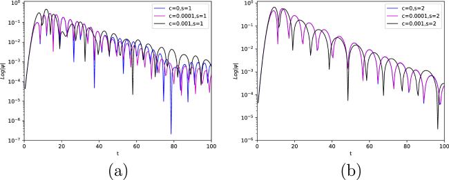
Figure 5. (a) The dynamical evolution of the nonlinear electrodynamics field in the background of the Bardeen–Kiselev BH spacetime (S = 1, ℓ = 3); (b) The dynamical evolution of gravitational perturbation in the background of the Bardeen–Kiselev BH spacetime (S = 2, ℓ = 2). In both cases, we take M = 1, q = 0.3, w = −2/3 and λ = 0.0003. |
5. Greybody factors and absorption coefficients
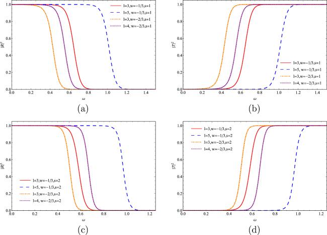
Figure 6. (a) The ∣R∣2 versus ω for electromagnetic perturbations; (b) ∣T∣2 vs ω for electromagnetic perturbations; (c) ∣R∣2 vs ω for gravitational perturbations; (d) ∣T∣2 vs ω for gravitational perturbations. In both cases, we take M = 1, q = 0.25, λ = 0.0025, c = 0.02, and electromagnetic perturbations (s = 1) and gravitational perturbations (s = 2). |
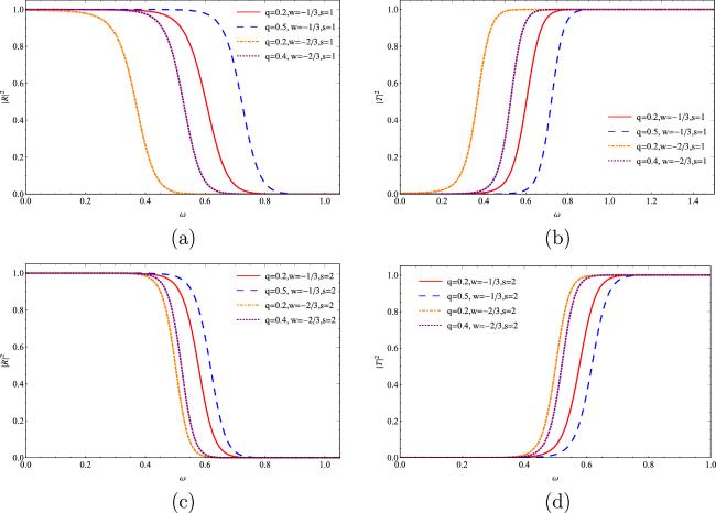
Figure 7. (a) The ∣R∣2 versus ω for electromagnetic perturbations; (b) ∣T∣2 vs ω for electromagnetic perturbations; (c) ∣R∣2 vs ω for gravitational perturbations; (d) ∣T∣2 vs ω for gravitational perturbations. In both cases, we take M = 1, ℓ = 3, λ = 0.0025, c = 0.02, and electromagnetic perturbations (s = 1) and gravitational perturbations (s = 2). |
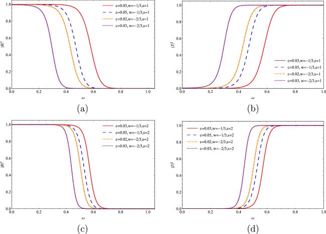
Figure 8. (a) The ∣R∣2 versus ω for electromagnetic perturbations; (b) ∣T∣2 vs ω for electromagnetic perturbations; (c) ∣R∣2 vs ω for gravitational perturbations; (d) ∣T∣2 vs ω for gravitational perturbations. In both cases, we take M = 1, ℓ = 3, λ = 0.0025, q = 0.25, and electromagnetic perturbations (s = 1) and gravitational perturbations (s = 2). |
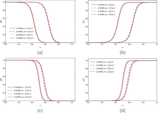
Figure 9. (a) The ∣R∣2 vs ω for electromagnetic perturbations; (b) ∣T∣2 vs ω for electromagnetic perturbations; (c) ∣R∣2 vs ω for gravitational perturbations; (d) ∣T∣2 vs ω for gravitational perturbations. In both cases, we take M = 1, ℓ = 3, q = 0.25, c = 0.02, and electromagnetic perturbations (s = 1) and gravitational perturbations (s = 2). |
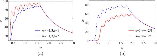
Figure 10. (a) The total absorption cross section (σ) vs ω for w = −1/3, M = 1, q = 0.25, λ = 0.0025 and c = 0.02; (b) The total absorption cross section (σ) vs ω for w = −2/3, q = 0.5, M = 1, c = 0.001 and λ = 0.0004. |
6. Conclusion
| 1. | 1. The value of the greybody bound is zero when the frequency is minimal, and the value of the greybody bound turns out to be 1 when the frequency is large enough, which implies that the wave is basically totally reflected when the frequency is small. Meanwhile, in view of the tunneling effect, a partial wave could pass through the potential barrier when the frequency increases, or the wave will not be reflected when the frequency reaches a certain level. |
| 2. | 2. Under electromagnetic and gravitational perturbations, for a fixed frequency, the responses of the greybody factor for different spacetime parameters are similar. |
| 3. | 3. Due to the presence of Kiselev quintessence, the transmission coefficient will increase. |