


1. Introduction
The problems of dark matter (DM) and dark energy revealed by astronomical observations posed major challenges to fundamental physics [1, 2]. There are two main approaches to understanding DM. In the first approach, one believes that DM is indeed some matter content in the Universe that has not yet been understood [3]. In the second approach, one speculates that DM is a sign that general relativity (GR) has to be modified at an astronomical scale. One should not ignore the fact that the problem of DM arises from the application of GR to the scale of the galaxy. In our current understanding of DM, it has the following characteristics. First, it neither radiates nor absorbs or reflects electromagnetic waves. Second, it only has gravitational interaction with baryonic matters. The above two characteristics look quite strange if DM is understood as real matter. In addition, up to now, it has not been possible to confirm the existence of DM in particle physics directly. Therefore, it is reasonable to consider the possibility that GR is no longer valid at the astronomical scale, and DM is nothing but spacetime geometry, which is strongly implied by the second characteristic of DM. From this perspective, modified gravitational theories, such as modified Newtonian dynamics [4], power-law f(R) theory [5], square-torsion theory [6], etc, are being employed to account for DM. We are not going to study the issue of DM from a phenomenological viewpoint. Rather, our purpose is to construct a fundamental theory of gravity with more degrees of freedom than those of GR from a geometrical viewpoint. As will be shown, so-called DM can naturally arise from the gravitational degrees of freedom in this theory.
On the one hand, the basic idea in GR is that so-called gravity is the geometry of spacetime, namely the effect of spacetime curvature. On the other hand, the localization of the Poincaré symmetry would naturally introduce both curvature and torsion as the fields strength of the gauge potentials [7]. Therefore, to combine the ideas of GR and gauge field theory, it is natural to construct a fundamental theory of gravity with both curvature and torsion. In this paper, the field equations of gravitational theory with torsion (GWT) will be proposed based on physically reasonable considerations. A spherically symmetric static vacuum solution of this theory will be studied. It turns out that certain DM can naturally arise from the gravitational degrees of freedom in this case. Throughout the paper, the geometric unit system [8] will be employed unless otherwise specified.
2. Gravitational theory with torsion
2.1. Basic principles
To generalize GR to GWT, we insist on the principles of general covariance and correspondence. The former requires that only dynamical variables can impact on the physical quantities in the expression of a physical law. The latter implies that the new GWT should return to GR when the spacetime torsion vanishes and hence all the experiments supporting GR would also support GWT.
It is well known that spacetime in GR has the structure of Riemannian geometry, where gravity is completely described by the curvature of spacetime. From a mathematical viewpoint, so-called Riemann–Cartan geometry is the minimal generalization of Riemannian geometry to include torsion [9, 10]. Thus, it is natural to consider Riemann–Cartan geometry as the spacetime geometry of GWT. Then a spacetime is a triple (M, gab, ∇c), where M denotes a 4-dimensional manifold, gab is a Lorentzian metric on M, and the covariant derivative operator ∇c is compatible with gab but not torsion-free. Hence, the torsion tensor ${T}_{\,\,{ab}}^{c}$ is included in the spacetime structure. For the convenience of expression, we will also use the unique torsion-free covariant derivative operator ${\tilde{{\rm{\nabla }}}}_{c}$ compatible with gab in some expressions. We assume that the world-line of a free particle is a time-like or null geodesic in (M, gab, ∇c) determined by the connection ∇c. The desired field equations of GWT will be proposed in the following subsections.
2.2. The implication of geodesic deviation
We consider only total-antisymmetric torsion in constructing our GWT. The reason emanates from the following observation on the definition of a separation vector for a geodesic deviation equation with torsion. Suppose that U is an open domain in (M, gab, ∇c) and there is a congruence of geodesics {γ(τ)} in U with proper time τ as the affine parameter. The tangent vectors ${Z}^{a}\equiv {\left(\tfrac{\partial }{\partial \tau }\right)}^{a}$ of the geodesics contribute a time-like vector field on U. Let μ0(s) be a smooth transverse curve, which is non-self-intersecting and the tangent vector ${w}^{a}\equiv {\left(\tfrac{\partial }{\partial s}\right)}^{a}$ at any point on μ0(s) is not tangent to the geodesic passing through that point, such that the geodesics can be labeled by γs(τ). By the actions of the one-parameter diffeomorphism group of the vector field Za, one can obtain a congruence of curves μτ(s), so that μτ(s) and γ(τ) form a 2-dimensional submanifold ${ \mathcal S }$ with coordinates τ and s. Then, on a reference observer's world-line, we have
$\begin{eqnarray}{Z}^{b}{{\rm{\nabla }}}_{b}({w}^{a}{Z}_{a})={Z}^{a}{Z}^{b}{T}_{({ab})c}{w}^{c},\end{eqnarray}$
where the torsion tensor ${T}_{\,\,{ab}}^{c}$ is defined by $({{\rm{\nabla }}}_{a}{{\rm{\nabla }}}_{b}-{{\rm{\nabla }}}_{b}{{\rm{\nabla }}}_{a})f=-{T}_{\,\,{ab}}^{c}{{\rm{\nabla }}}_{c}f$ with f being any smooth scalar field on M. Therefore, for a general torsion, the separation vector wa cannot remain as a spatial vector orthogonal to Za along the reference observer's world-line. The necessary and sufficient condition to employ wa as the spatial separation vector is Zb∇b(waZa) = 0. This requirement is equivalent to $\begin{eqnarray}{Z}^{a}{Z}^{b}{T}_{({ab})c}{w}^{c}=0,\quad \forall \,{Z}^{a}.\end{eqnarray}$
From this perspective, it is natural to consider the torsion satisfying Tabc = T[ab]c. Since the torsion itself satisfies Tabc = Ta[bc], the above requirement leads to Tabc = T[abc]. It should be noted that a geodesic in Riemann–Cartan space with totally antisymmetric torsion coincides with that in Riemann space, which is determined by the metric.Based on the above assumption of totally antisymmetric torsion, we now infer the field equation for GWT. In the proper coordinate system {xμ} of the reference observer in geodesic congruence, one can define the 3-velocity and 3-acceleration of a nearby geodesic as ${u}^{b}:= {Z}^{a}{\partial }_{a}{w}^{b}={Z}^{a}{{\rm{\nabla }}}_{a}{w}^{b}-\tfrac{1}{2}{T}_{\,\,{ac}}^{b}{Z}^{a}{w}^{c}$, and ${a}^{c}:= {Z}^{a}{\partial }_{a}{u}^{c}={Z}^{a}{{\rm{\nabla }}}_{a}{u}^{c}-\tfrac{1}{2}{T}_{\,\,{ab}}^{c}{Z}^{a}{u}^{b}$, where ∂a denotes the coordinate derivative. Then in (M, gab, ∇c), we obtain the following geodesic deviation equation3 ) and (4 ) implies the following correspondence:6 ) is to assume the following equation:7 ) and (8 ), we infer the following field equation:9 ) gives7 ) can be derived from equations (9 ) and (10 ).
$\begin{eqnarray}\begin{array}{rcl}{a}^{c} & = & -{{R}_{{abd}}}^{c}{Z}^{a}{w}^{b}{Z}^{d}+\displaystyle \frac{1}{2}{Z}^{a}{w}^{b}{Z}^{d}{{\rm{\nabla }}}_{d}{T}_{\,\,{ab}}^{c}\\ & & +\displaystyle \frac{1}{4}{T}_{\,\,{ae}}^{c}{T}_{\,\,{db}}^{e}{Z}^{a}{Z}^{d}{w}^{b}.\end{array}\end{eqnarray}$
It is well known that the tidal acceleration in Newtonian gravity can be expressed as $\begin{eqnarray}{a}^{c}=-{w}^{b}{\partial }_{b}{\partial }^{c}\phi ,\end{eqnarray}$
where φ is the gravitational potential. The comparison between equations ( $\begin{eqnarray}{{R}_{{abd}}}^{c}{Z}^{a}{Z}^{d}-\displaystyle \frac{1}{2}{Z}^{a}{Z}^{d}{{\rm{\nabla }}}_{d}{T}_{\,\,{ab}}^{c}-\displaystyle \frac{1}{4}{T}_{\,\,{ae}}^{c}{T}_{\,\,{db}}^{e}{Z}^{a}{Z}^{d}\,\longleftrightarrow \,{\partial }_{b}{\partial }^{c}\phi ,\end{eqnarray}$
and hence $\begin{eqnarray}\begin{array}{l}{R}_{{ab}}{Z}^{a}{Z}^{b}+\displaystyle \frac{1}{4}{{T}^{{cd}}}_{a}{T}_{{bcd}}{Z}^{a}{Z}^{b}\,\longleftrightarrow \,{\partial }_{b}{\partial }^{b}\phi =4\pi \rho \\ \quad =\,4\pi {S}_{{ab}}{Z}^{a}{Z}^{b},\end{array}\end{eqnarray}$
where Sab represents the energy-momentum tensor of the matter field, which also contains the contribution of DM and dark energy in the context of GR. On one hand, a direct realisation of the correspondence equation ( $\begin{eqnarray}{R}_{{ab}}{Z}^{a}{Z}^{b}+\displaystyle \frac{1}{4}{{T}^{{cd}}}_{a}{T}_{{bcd}}{Z}^{a}{Z}^{b}=4\pi {S}_{{ab}}{Z}^{a}{Z}^{b}.\end{eqnarray}$
On the other hand, the total energy-momentum is supposed to satisfy the constraint of the conservation law ${\tilde{{\rm{\nabla }}}}^{a}{S}_{{ab}}=0$, where ${\tilde{{\rm{\nabla }}}}_{a}$ denotes the torsion-free covariant derivative determined by the metric. Note that the Bianchi identity with torsion reads ${{\rm{\nabla }}}_{[a}{{R}_{{bc}]d}}^{e}={T}_{\,\,[{ab}}^{f}{{R}_{c]{fd}}}^{e}$. Given the premise of totally antisymmetric torsion, it can be reduced to $\begin{eqnarray}{\tilde{{\rm{\nabla }}}}^{a}\left({G}_{{ab}}+\eta {g}_{{ab}}+\frac{1}{4}{{T}^{{cd}}}_{a}{T}_{{bcd}}\right)=0,\end{eqnarray}$
where ${G}_{{ab}}\equiv {R}_{{ab}}-\tfrac{1}{2}{{Rg}}_{{ab}}$ and $\eta \equiv -\tfrac{1}{8}{T}_{{cab}}{T}^{{cab}}$. Based on equations ( $\begin{eqnarray}{R}_{{ab}}-\displaystyle \frac{1}{2}{{Rg}}_{{ab}}+\eta {g}_{{ab}}+\displaystyle \frac{1}{4}{{T}^{{cd}}}_{a}{T}_{{bcd}}=8\pi {S}_{{ab}}.\end{eqnarray}$
It is easy to check that equation ( $\begin{eqnarray}R=2\eta -8\pi S,\end{eqnarray}$
where S ≡ gabSab. Thus, in the Newtonian approximation, one has S ≈ –ρ, equation (Let ${\tilde{R}}_{{ab}}$ be the Ricci tensor determined by the metric or ${\tilde{{\rm{\nabla }}}}_{a}$. Then, for a totally antisymmetric torsion, one has ${R}_{{ab}}={\tilde{R}}_{{ab}}+\tfrac{1}{2}{\tilde{{\rm{\nabla }}}}_{c}{T}_{\,\,{ab}}^{c}-\tfrac{1}{4}{{T}^{{cd}}}_{a}{T}_{{bcd}}$ and $R=\tilde{R}-\tfrac{1}{4}{T}_{{cab}}{T}^{{cab}}$. By substituting them into equation (9 ), we obtain11 ) implies that the energy-momentum tensor Sab which we employed is not symmetric with respect to its indices. Therefore, the properties of both the geometry and matter fields in our theory have been extended beyond the scope of GR.
$\begin{eqnarray}{\tilde{G}}_{{ab}}+\displaystyle \frac{1}{2}{\tilde{{\rm{\nabla }}}}_{c}{T}_{\,\,{ab}}^{c}=8\pi {S}_{{ab}},\end{eqnarray}$
where ${\tilde{G}}_{{ab}}$ represents the Einstein tensor determined by the metric. Equation (2.3. The degree freedom of gravity and the energy-momentum of matter
Let us consider whether equation (11 ) could be a suitable field equation for GWT. The metric tensor gab has 10 independent degrees of freedom, while the totally antisymmetric torsion Tcab, as a 3-form, has 4 independent degrees of freedom. Thus, the spacetime geometry contains 14 independent degrees of freedom. However, the energy-momentum Sab is the most general (0, 2)-type tensor and has 16 independent components. Therefore, equation (11 ) is over-constrained in the most general case. To make equation (11 ) mathematically solvable, two new scalar field degrees of freedom of gravity have to be added. A core idea of this paper is that so-called DM and dark energy come from the gravitational degrees of freedom. Therefore, we assume that Sab can be divided into two parts,
$\begin{eqnarray}{S}_{{ab}}={\breve{{\rm{\Sigma }}}}_{{ab}}-\displaystyle \frac{1}{8\pi }{X}_{{ab}},\end{eqnarray}$
where Xab ≡ Xab[gab, Tcab, Λ, Φ] is a local function of gab, Tcab, Λ and Φ, and may play the roles of DM and dark energy, and ${\breve{{\rm{\Sigma }}}}_{{ab}}$ represents the energy-momentum tensor of a real matter field. Taking account of the fact that dark energy behaves like a cosmological constant, for simplicity we assume that Xab is a linear combination of the terms Λgab, ${{T}^{{cd}}}_{a}{T}_{{bcd}}$ and $({\tilde{{\rm{\nabla }}}}_{c}{\rm{\Phi }}){T}_{\,\,{ab}}^{c}$ with the following ‘chain coupling': $\begin{eqnarray*}{\rm{\Lambda }}\mathop{\longleftrightarrow }\limits^{{\rm{\Lambda }}{g}_{{ab}}}{g}_{{ab}}\mathop{\longleftrightarrow }\limits^{{{T}^{{cd}}}_{a}{T}_{{bcd}}}{T}_{{cab}}\mathop{\longleftrightarrow }\limits^{({\tilde{{\rm{\nabla }}}}_{c}{\rm{\Phi }}){T}_{\,\,{ab}}^{c}}{\rm{\Phi }},\end{eqnarray*}$
i.e. $\begin{eqnarray}{X}_{{ab}}={\rm{\Lambda }}{g}_{{ab}}+{T}_{\,\,\,\,a}^{{cd}}{T}_{{bcd}}+({\tilde{{\rm{\nabla }}}}_{c}{\rm{\Phi }}){T}_{\,\,{ab}}^{c}.\end{eqnarray}$
Next, we consider the energy-momentum tensor ${\breve{{\rm{\Sigma }}}}_{{ab}}$ of the real matter field. In GWT, it is reasonable to assume that the real matter field $\Psi$ should be coupled to both the metric and the torsion. Thus ${\breve{{\rm{\Sigma }}}}_{{ab}}$ is a local function of $\Psi$, gab and ${T}_{\,\,{ab}}^{c}$. By generalizing the Belinfante energy-momentum tensor ${E}_{{ab}}^{{\mathscr{B}}}$ in GR [11], we define ${\breve{{\rm{\Sigma }}}}_{{ab}}$ as
$\begin{eqnarray}{\breve{{\rm{\Sigma }}}}^{{ab}}:= {{\rm{\Sigma }}}^{{ab}}-{\tilde{{\rm{\nabla }}}}_{c}({\tau }^{{cab}}-{\tau }^{{bca}}+{\tau }^{{abc}}),\end{eqnarray}$
where $\begin{eqnarray*}{{\rm{\Sigma }}}^{{ab}}:= -\displaystyle \frac{\partial { \mathcal L }}{\partial {\tilde{{\rm{\nabla }}}}_{a}{\rm{\Psi }}}{\tilde{{\rm{\nabla }}}}^{b}{\rm{\Psi }}+{g}^{{ab}}{ \mathcal L },\quad {\tau }^{{cab}}:= -\displaystyle \frac{\partial { \mathcal L }}{\partial {\tilde{{\rm{\nabla }}}}_{c}{\rm{\Psi }}}{\hat{{\rm{\Psi }}}}^{[{ab}]}.\end{eqnarray*}$
Here, ${ \mathcal L }\equiv { \mathcal L }({\rm{\Psi }},{{\rm{\nabla }}}_{a}{\rm{\Psi }},{g}_{{ab}})$ is the Lagrangian density of the real matter field in GWT, and ${\hat{{\rm{\Psi }}}}_{\,b}^{a}$ is the simple notation for ${\hat{{\rm{\Psi }}}}_{\,\,\,\,\,\,\,\,{d}_{1}\cdots {d}_{l}\,\,b}^{{c}_{1}\cdots {c}_{k}\,\,\,\,\,\,\,\,a}={\sum }_{i=1}^{k}{{\rm{\Psi }}}_{\qquad \,\,\,\,\,\,\,\,{d}_{1}\cdots {d}_{l}}^{{c}_{1}\cdots a\cdots {c}_{k}}{\delta }_{\,\,b}^{{c}_{i}}-{\sum }_{j=1}^{l}{{\rm{\Psi }}}_{\,\,\,\,\,\,\,\,{d}_{1}\cdots b\cdots {d}_{l}}^{{c}_{1}\cdots {c}_{k}}{\delta }_{\,\,{d}_{j}}^{a}$. It is obvious from the definition of ${\breve{{\rm{\Sigma }}}}^{{ab}}$ that it reduces to ${E}_{{ab}}^{{\mathscr{B}}}$ for a vanishing torsion.We assume that the Lagrangian of the matter field can be written as a sum of the torsion-free part and torsion part, i.e. ${ \mathcal L }=\tilde{{ \mathcal L }}+\bar{{ \mathcal L }}$, so is the energy-momentum,
$\begin{eqnarray}{\breve{{\rm{\Sigma }}}}^{{ab}}={\tilde{E}}^{{ab}}+{\bar{E}}^{{ab}},\end{eqnarray}$
where $\begin{eqnarray*}{\tilde{E}}^{{ab}}:= {\tilde{{\rm{\Sigma }}}}^{{ab}}-{\tilde{{\rm{\nabla }}}}_{c}({\tilde{\tau }}^{{cab}}-{\tilde{\tau }}^{{bca}}+{\tilde{\tau }}^{{abc}}),\end{eqnarray*}$
with $\begin{eqnarray*}{\tilde{{\rm{\Sigma }}}}^{{ab}}:= -\displaystyle \frac{\partial \tilde{{ \mathcal L }}}{\partial {\tilde{{\rm{\nabla }}}}_{a}{\rm{\Psi }}}{\tilde{{\rm{\nabla }}}}^{b}{\rm{\Psi }}+{g}^{{ab}}\tilde{{ \mathcal L }},\quad {\tilde{\tau }}^{{cab}}:= -\displaystyle \frac{\partial \tilde{{ \mathcal L }}}{\partial {\tilde{{\rm{\nabla }}}}_{c}{\rm{\Psi }}}{\hat{{\rm{\Psi }}}}^{[{ab}]},\end{eqnarray*}$
and $\begin{eqnarray*}{\bar{E}}^{{ab}}:= {\bar{{\rm{\Sigma }}}}^{{ab}}-{\tilde{{\rm{\nabla }}}}_{c}({\bar{\tau }}^{{cab}}-{\bar{\tau }}^{{bca}}+{\bar{\tau }}^{{abc}}),\end{eqnarray*}$
with $\begin{eqnarray*}{\bar{{\rm{\Sigma }}}}^{{ab}}:= -\displaystyle \frac{\partial \bar{{ \mathcal L }}}{\partial {\tilde{{\rm{\nabla }}}}_{a}{\rm{\Psi }}}{\tilde{{\rm{\nabla }}}}^{b}{\rm{\Psi }}+{g}^{{ab}}\bar{{ \mathcal L }},\quad {\bar{\tau }}^{{cab}}:= -\displaystyle \frac{\partial \bar{{ \mathcal L }}}{\partial {\tilde{{\rm{\nabla }}}}_{c}{\rm{\Psi }}}{\hat{{\rm{\Psi }}}}^{[{ab}]}.\end{eqnarray*}$
Let ${\tilde{E}}_{({ab})}$ and ${\tilde{E}}_{[{ab}]}$ represent the symmetric and antisymmetric parts of ${\tilde{E}}_{{ab}}$, respectively, defined by ${\tilde{E}}_{({ab})}:= \tfrac{1}{2}({\tilde{E}}_{{ab}}+{\tilde{E}}_{{ba}})$ and ${\tilde{E}}_{[{ab}]}:= \tfrac{1}{2}({\tilde{E}}_{{ab}}-{\tilde{E}}_{{ba}})$. Then one has $\begin{eqnarray}\begin{array}{rcl}{\breve{{\rm{\Sigma }}}}_{{ab}} & = & {\breve{{\rm{\Sigma }}}}_{({ab})}+{\breve{{\rm{\Sigma }}}}_{[{ab}]}\\ & = & {\tilde{E}}_{({ab})}+{\bar{E}}_{({ab})}+{\tilde{E}}_{[{ab}]}+{\bar{E}}_{[{ab}]}.\end{array}\end{eqnarray}$
2.4. The field equations for GWT and related issues
By substituting equations (12 ), (13 ) and (16 ) into equation (11 ) and dividing the result into its symmetric and antisymmetric parts, we obtain the following two field equations:17 ) and (18 ), we get18 ) and (20 ) vanish, and equations (17 ) and (19 ) reduce to22 ) shows that Λ is a constant. Therefore, equation (21 ) can be rewritten as ${\tilde{G}}_{{ab}}+\tilde{{\rm{\Lambda }}}{g}_{{ab}}=8\pi {E}_{{ab}}^{{\mathscr{B}}}$, which is exactly the Einstein field equation (with or without a cosmological constant). Therefore, the scalar field Λ in GWT can be regarded as a dynamical generalization of the non-dynamical cosmological constant $\tilde{{\rm{\Lambda }}}$ in GR.
$\begin{eqnarray}{\tilde{G}}_{{ab}}+{\rm{\Lambda }}{g}_{{ab}}+{{T}^{{cd}}}_{a}{T}_{{bcd}}=8\pi \left({\tilde{E}}_{({ab})}+{\bar{E}}_{({ab})}\right),\end{eqnarray}$
$\begin{eqnarray}\displaystyle \frac{1}{2}{\tilde{{\rm{\nabla }}}}_{c}{T}_{\,\,{ab}}^{c}+({\tilde{{\rm{\nabla }}}}_{c}{\rm{\Phi }}){T}_{\,\,{ab}}^{c}=8\pi \left({\tilde{E}}_{[{ab}]}+{\bar{E}}_{[{ab}]}\right).\end{eqnarray}$
By applying the torsion-free covariant derivative operator ${\tilde{{\rm{\nabla }}}}^{a}$ to equations ( $\begin{eqnarray}{\tilde{{\rm{\nabla }}}}_{b}{\rm{\Lambda }}+{\tilde{{\rm{\nabla }}}}^{a}({{T}^{{cd}}}_{a}{T}_{{bcd}})=8\pi {\tilde{{\rm{\nabla }}}}^{a}\left({\tilde{E}}_{({ab})}+{\bar{E}}_{({ab})}\right),\end{eqnarray}$
$\begin{eqnarray}{\tilde{{\rm{\nabla }}}}^{a}[({\tilde{{\rm{\nabla }}}}_{c}{\rm{\Phi }}){T}_{\,\,{ab}}^{c}]=8\pi {\tilde{{\rm{\nabla }}}}^{a}\left({\tilde{E}}_{[{ab}]}+{\bar{E}}_{[{ab}]}\right),\end{eqnarray}$
respectively. In the case of ${T}_{\,\,{ab}}^{c}=0$, equations ( $\begin{eqnarray}{\tilde{G}}_{{ab}}+{\rm{\Lambda }}{g}_{{ab}}=8\pi {E}_{{ab}}^{{\mathscr{B}}},\end{eqnarray}$
$\begin{eqnarray}{\tilde{{\rm{\nabla }}}}_{b}{\rm{\Lambda }}=8\pi {\tilde{{\rm{\nabla }}}}^{a}{E}_{{ab}}^{{\mathscr{B}}}=0,\end{eqnarray}$
respectively. Equation (In the vacuum case ($\Psi$ = 0), equation (17 ) can be rewritten as23 ) can be regarded as the Einstein equation in GR with certain effective ‘matter' whose energy-momentum tensor is described by Pab. Let us consider the properties of Pab. Let Ua be the normalized 4-velocity of an observer, with its spatial projection ${h}_{\,\,\,b}^{a}\equiv {\delta }_{\,\,b}^{a}+{U}^{a}{U}_{b}$. Let ${{\mathfrak{t}}}_{a}\equiv {\left({}^{{\boldsymbol{* }}}T\right)}_{a}$ be the Hodge dual of the 3-form Tcab. We define Ω ≡ TcabTcab, $\vartheta \equiv {U}_{a}{{\mathfrak{t}}}^{a}$ and ${\bar{{\mathfrak{t}}}}^{a}\equiv {{h}^{a}}_{b}{{\mathfrak{t}}}^{b}$. Then, Pab can be expressed as
$\begin{eqnarray}{\tilde{G}}_{{ab}}=8\pi {P}_{{ab}},\end{eqnarray}$
where ${P}_{{ab}}\equiv -\left(\tfrac{1}{8\pi }{{T}^{{cd}}}_{a}{T}_{{bcd}}+\tfrac{{\rm{\Lambda }}}{8\pi }{g}_{{ab}}\right)$ comes from the gravitational degrees of freedom. Thus, equation ( $\begin{eqnarray}{P}_{{ab}}=\bar{\rho }{U}_{a}{U}_{b}+\bar{p}{h}_{{ab}}+{U}_{(a}{\bar{q}}_{b)}+{\bar{\zeta }}_{{ab}},\end{eqnarray}$
where $\bar{\rho }\equiv \tfrac{1}{8\pi }(\tfrac{1}{3}{\rm{\Omega }}+{\rm{\Lambda }}-2{\vartheta }^{2})$, $\bar{p}\equiv -\tfrac{1}{8\pi }(\tfrac{1}{3}{\rm{\Omega }}+{\rm{\Lambda }})$, ${\bar{q}}_{a}\,\equiv \tfrac{\vartheta }{2\pi }{\bar{{\mathfrak{t}}}}_{a}$, and ${\bar{\zeta }}_{{ab}}\equiv -\tfrac{1}{4\pi }{\bar{{\mathfrak{t}}}}_{a}{\bar{{\mathfrak{t}}}}_{b}$. By thinking of Pab as the energy-momentum tensor of a fluid, $\bar{\rho }$, $\bar{p}$, ${\bar{q}}_{a}$ and ${\bar{\zeta }}_{{ab}}$ denote its mass density, pressure, heat flow and stress respectively, though the so-called matter described by Pab originates from the gravity in GWT. Thus, it is possible that the effective matter can play the role of DM or dark energy.3. Spherically symmetric static vacuum solution of GWT
In the GWT constructed in the previous section, in addition to the spacetime metric gab, extra fields Λ, Φ and ${T}_{\,\,{ab}}^{c}$ are introduced to describe the gravitational degrees of freedom. Therefore, a killing vector field ξa should satisfy that the Lie derivatives of all the gravitational fields in GWT vanish. In GR, there are the following four killing vector fields to characterize the static spherical symmetric metric,17 ) and (18 ), the vacuum field equations of GWT read26 ) yields the following system of differential equations,27 ) provides the differential equation
$\begin{eqnarray*}\begin{array}{rcl}{\xi }_{0}^{\,a} & = & {\left(\displaystyle \frac{\partial }{\partial t}\right)}^{a},\quad {\xi }_{2}^{\,a}=\sin \varphi {\left(\displaystyle \frac{\partial }{\partial \theta }\right)}^{a}+\cot \theta \cos \varphi {\left(\displaystyle \frac{\partial }{\partial \varphi }\right)}^{a},\\ {\xi }_{1}^{\,a} & = & {\left(\displaystyle \frac{\partial }{\partial \varphi }\right)}^{a},\,\,{\xi }_{3}^{\,a}=\cos \varphi {\left(\displaystyle \frac{\partial }{\partial \theta }\right)}^{a}-\cot \theta \sin \varphi {\left(\displaystyle \frac{\partial }{\partial \varphi }\right)}^{a},\end{array}\end{eqnarray*}$
in the Schwarzschild coordinate system {t, r, θ, φ}. For the symmetric solutions of GWT with the above killing vectors, the static spherically symmetric line element is expressed as $\begin{eqnarray*}{\rm{d}}{s}^{2}=-{{\rm{e}}}^{2A(r)}{\rm{d}}{t}^{2}+{{\rm{e}}}^{2B(r)}{\rm{d}}{r}^{2}+{r}^{2}({\rm{d}}{\theta }^{2}+{\sin }^{2}\theta {\rm{d}}{\varphi }^{2}),\end{eqnarray*}$
where A(r) and B(r) are undetermined functions. The scalar fields Λ, Φ and totally antisymmetric torsion ${T}_{\,\,{ab}}^{c}$ take the forms Λ = Λ(r), Φ = Φ(r) and $\begin{eqnarray}{{\mathfrak{t}}}^{a}=\displaystyle \frac{{\mathsf{d}}(r)}{{\boldsymbol{c}}}{\left(\displaystyle \frac{\partial }{\partial t}\right)}^{a}-C(r){\left(\displaystyle \frac{\partial }{\partial r}\right)}^{a},\end{eqnarray}$
respectively, where c is the speed of light in vacuum, C(r) and d(r) are two undetermined functions whose dimensions read $[{\mathsf{d}}(r)]={\left[L\right]}^{-1}=[C(r)]$, with [L] denoting the length dimension. Hereafter, we employ the international system of units instead of the geometric system for convenience. From equations ( $\begin{eqnarray}{\tilde{G}}_{{ab}}+{\rm{\Lambda }}{g}_{{ab}}+{{T}^{{cd}}}_{a}{T}_{{bcd}}=0,\end{eqnarray}$
$\begin{eqnarray}\displaystyle \frac{1}{2}{\tilde{{\rm{\nabla }}}}_{c}{T}_{\,\,{ab}}^{c}+({\tilde{{\rm{\nabla }}}}_{c}{\rm{\Phi }}){T}_{\,\,{ab}}^{c}=0.\end{eqnarray}$
In the static spherically symmetric case, equation ( $\begin{eqnarray}{CD}=0,\end{eqnarray}$
$\begin{eqnarray}\begin{array}{l}-{A}^{{\prime\prime} }+{A}^{{\prime} }{B}^{{\prime} }-{A}^{{\prime} 2}-\displaystyle \frac{2{A}^{{\prime} }}{r}-({{\rm{e}}}^{2A}{D}^{2}\\ \quad -\,{{\rm{e}}}^{2B}{C}^{2}+{\rm{\Lambda }}){{\rm{e}}}^{2B}-2{D}^{2}{{\rm{e}}}^{2(A+B)}=0,\end{array}\end{eqnarray}$
$\begin{eqnarray}\begin{array}{l}-\,{A}^{{\prime\prime} }+{A}^{{\prime} }{B}^{{\prime} }-{A}^{{\prime} 2}+\displaystyle \frac{2{B}^{{\prime} }}{r}-({{\rm{e}}}^{2A}{D}^{2}\\ \quad -\,{{\rm{e}}}^{2B}{C}^{2}+{\rm{\Lambda }}){{\rm{e}}}^{2B}+2{C}^{2}{{\rm{e}}}^{4B}=0,\end{array}\end{eqnarray}$
$\begin{eqnarray}\begin{array}{l}-\,\frac{1}{{{\rm{e}}}^{2B}}\left[1+r({A}^{{\prime} }-{B}^{{\prime} })\right]+1\\ \quad -\,({{\rm{e}}}^{2A}{D}^{2}-{{\rm{e}}}^{2B}{C}^{2}+{\rm{\Lambda }}){r}^{2}=0,\end{array}\end{eqnarray}$
where the notation $\,^{\prime} \,$ denotes the derivative with respect to r. Simultaneously, equation ( $\begin{eqnarray}\displaystyle \frac{1}{2}{D}^{{\prime} }+D({A}^{{\prime} }+{{\rm{\Phi }}}^{{\prime} })=0,\end{eqnarray}$
where $D(r)\equiv \tfrac{{\mathsf{d}}(r)}{{\boldsymbol{c}}}$.Notice that equation (28 ) has three possible solutions: (C = 0, D = 0), (C ≠ 0, D = 0) and (C = 0, D ≠ 0). Note that nontrivial torsion appears in the latter two cases. In the third case where the torsion vector ${{\mathfrak{t}}}^{a}$ has only a time component, equation (24 ) simplifies to ${P}_{{ab}}=\bar{\rho }{U}_{a}{U}_{b}+\bar{p}{h}_{{ab}}$, and hence the effective matter looks like a ‘perfect fluid'. This is the case which we will study in detail. For simplicity, we consider the special case that ${{\mathfrak{t}}}^{a}$ is a constant vector and ${{\rm{\Phi }}}^{{\prime} }=-{A}^{{\prime} }$. Then equation (32 ) yields $D=\tfrac{{\mathsf{d}}}{{\boldsymbol{c}}}$, where d is an undetermined dimensional constant. Hence, by equations (29 ), (30 ) and (31 ), we obtain34 ) and (33 ) to obtain34 ), (35 ) and (36 ), we can derive the differential equation which f satisfies as35 ) that
$\begin{eqnarray}-{A}^{{\prime\prime} }+{A}^{{\prime} }{B}^{{\prime} }-{A}^{{\prime} 2}-\displaystyle \frac{2{A}^{{\prime} }}{r}-\displaystyle \frac{3{{\mathsf{d}}}^{2}}{{{\boldsymbol{c}}}^{2}}{{\rm{e}}}^{2(A+B)}-{\rm{\Lambda }}{{\rm{e}}}^{2B}=0,\end{eqnarray}$
$\begin{eqnarray}-{A}^{{\prime\prime} }+{A}^{{\prime} }{B}^{{\prime} }-{A}^{{\prime} 2}+\displaystyle \frac{2{B}^{{\prime} }}{r}-\displaystyle \frac{{{\mathsf{d}}}^{2}}{{{\boldsymbol{c}}}^{2}}{{\rm{e}}}^{2(A+B)}-{\rm{\Lambda }}{{\rm{e}}}^{2B}=0,\end{eqnarray}$
$\begin{eqnarray}\displaystyle \frac{{{\rm{e}}}^{2B}-1}{{r}^{2}}-\displaystyle \frac{{A}^{{\prime} }-{B}^{{\prime} }}{r}-\displaystyle \frac{{{\mathsf{d}}}^{2}}{{{\boldsymbol{c}}}^{2}}{{\rm{e}}}^{2(A+B)}-{\rm{\Lambda }}{{\rm{e}}}^{2B}=0.\end{eqnarray}$
Letting f ≡ e2A and g ≡ e2B, we can integrate the difference between equations ( $\begin{eqnarray}{fg}=\displaystyle \frac{{{\boldsymbol{c}}}^{2}}{{{\mathsf{d}}}^{2}}\displaystyle \frac{1}{{r}^{2}+{\beta }^{2}},\end{eqnarray}$
where β is an integral constant with a length dimension. From equations ( $\begin{eqnarray}\begin{array}{l}\displaystyle \frac{{{\rm{d}}}^{2}f}{{\rm{d}}{r}^{2}}+\displaystyle \frac{r}{{r}^{2}+{\beta }^{2}}\displaystyle \frac{{\rm{d}}f}{{\rm{d}}r}+\left(\displaystyle \frac{2}{{r}^{2}+{\beta }^{2}}-\displaystyle \frac{2}{{r}^{2}}\right)\,f\\ =-\displaystyle \frac{2{{\boldsymbol{c}}}^{2}}{{{\mathsf{d}}}^{2}}\displaystyle \frac{1}{{r}^{2}}\displaystyle \frac{1}{{r}^{2}+{\beta }^{2}}.\end{array}\end{eqnarray}$
Additionally, it can be deduced from equation ( $\begin{eqnarray}{\rm{\Lambda }}=\displaystyle \frac{1}{{r}^{2}}\left(1-\displaystyle \frac{1}{g}\right)-\displaystyle \frac{1}{r}\left(\displaystyle \frac{{f}^{{\prime} }}{2f}-\displaystyle \frac{{g}^{{\prime} }}{2g}\right)\displaystyle \frac{1}{g}-\displaystyle \frac{{{\mathsf{d}}}^{2}}{{{\boldsymbol{c}}}^{2}}f.\end{eqnarray}$
By careful observation of equation (37 ), we notice that its solution would contain a transcendental function of the coordinate r. Hence, we multiply equation (37 ) by $\tfrac{1}{{{\mathsf{d}}}^{2}}$ and define the dimensionless variable x ≡ ∣d∣ · r. Then, equation (37 ) becomes39 ) reads
$\begin{eqnarray}\begin{array}{l}\displaystyle \frac{{{\rm{d}}}^{2}f}{{\rm{d}}{x}^{2}}+\displaystyle \frac{x}{{x}^{2}+{\left({\mathsf{d}}\beta \right)}^{2}}\displaystyle \frac{{\rm{d}}f}{{\rm{d}}x}+\left[\displaystyle \frac{2}{{x}^{2}+{\left({\mathsf{d}}\beta \right)}^{2}}-\displaystyle \frac{2}{{x}^{2}}\right]\,f\\ =-2{{\boldsymbol{c}}}^{2}\displaystyle \frac{1}{{x}^{2}}\displaystyle \frac{1}{{x}^{2}+{\left({\mathsf{d}}\beta \right)}^{2}}.\end{array}\end{eqnarray}$
The general solution of equation ( $\begin{eqnarray}\begin{array}{l}f\equiv f(x)=f(| {\mathsf{d}}| r)=\displaystyle \frac{{{\boldsymbol{c}}}^{2}}{{\left({\mathsf{d}}\beta \right)}^{2}}+\alpha \displaystyle \frac{\sqrt{{x}^{2}+{\left({\mathsf{d}}\beta \right)}^{2}}}{x}\\ \quad +\gamma \left\{\displaystyle \frac{\sqrt{{x}^{2}+{\left({\mathsf{d}}\beta \right)}^{2}}}{x}\mathrm{ln}\left[x+\sqrt{{x}^{2}+\,{\left({\mathsf{d}}\beta \right)}^{2}}\right]-1\right\},\end{array}\end{eqnarray}$
where α and γ are integral constants whose dimensions read $[\alpha ]={\left[L\right]}^{2}{\left[T\right]}^{-2}=[\gamma ]$, where [T] represents the time dimension.By setting the integration constant $\beta =\tfrac{1}{{\mathsf{d}}}$ in equation (40 ), we obtain41 ) for small x. In this case, one has $\tfrac{\sqrt{{x}^{2}+1}}{x}\,\approx \tfrac{1}{x}=\tfrac{1}{| {\mathsf{d}}| r}$ and $\tfrac{\sqrt{{x}^{2}+1}}{x}\mathrm{arsinh}\,x-1\approx \tfrac{\mathrm{ln}(x+1)}{x}-1\approx 0$. By setting the integration constant α = –2GM∣d∣, where G is the gravitational constant and M is a quantity with mass dimension, equation (41 ) yields $f\approx \left(1-\tfrac{2{GM}}{{{\boldsymbol{c}}}^{2}r}\right){{\boldsymbol{c}}}^{2}$, and, further, equation (36 ) implies $g\approx {\left(1-\tfrac{2{GM}}{{{\boldsymbol{c}}}^{2}r}\right)}^{-1}$. Hence, the approximation of the solution corresponds to the Schwarzschild solution in GR. It should be noted that this setting of α coincides with its dimension as $[-2{GM}| {\mathsf{d}}| ]={\left[L\right]}^{2}{\left[T\right]}^{-2}$. To see whether the solution of equations (36 ) and (41 ) can be used to explain a galactic rotation curve, we note that the rotational velocity of a test body can be expressed as ${v}^{2}(r)=r\tfrac{\partial \phi }{\partial r}$, where $\phi \equiv -\tfrac{{{\boldsymbol{c}}}^{2}}{2}\left(1+\tfrac{1}{{{\boldsymbol{c}}}^{2}}{g}_{00}\right)$ represents the gravitational potential expressed by the metric component. Hence, equation (41 ) implies
$\begin{eqnarray}f(x)={{\boldsymbol{c}}}^{2}+\alpha \displaystyle \frac{\sqrt{{x}^{2}+1}}{x}+\gamma \left(\displaystyle \frac{\sqrt{{x}^{2}+1}}{x}\mathrm{arsinh}\,x-1\right).\end{eqnarray}$
Note that in the limit of vanishing torsion, the GWT should return to GR. To check this, we consider the behavior of solution ( $\begin{eqnarray}{v}^{2}(r)=-\displaystyle \frac{\alpha }{2}\displaystyle \frac{1}{x\sqrt{{x}^{2}+1}}-\displaystyle \frac{\gamma }{2}\left(\displaystyle \frac{\mathrm{arsinh}\,x}{x\sqrt{{x}^{2}+1}}-1\right).\end{eqnarray}$
Therefore the asymptotic velocity vc satisfies $\begin{eqnarray}{v}_{c}^{2}\equiv \mathop{\mathrm{lim}}\limits_{x\to +\infty }{v}^{2}(r)=\displaystyle \frac{\gamma }{2},\end{eqnarray}$
which coincides with the asymptotic behavior of a galactic rotation curve [12]. According to the baryonic Tully–Fisher relation, which is a widely verified empirical relationship between the mass of a spiral galaxy and its asymptotic rotation velocity [13], $\begin{eqnarray}M=\kappa {v}_{c}^{4},\end{eqnarray}$
where $\kappa \approx 35{h}_{75}^{-2}{M}_{\odot }{\mathrm{km}}^{-4}\cdot {{\rm{s}}}^{4}$, M⊙ and h75 are the solar mass and the dimensionless Hubble constant respectively, the integral constant can be fixed as $\gamma =2\sqrt{\tfrac{M}{\kappa }}$.By substituting α = − 2GM∣d∣, $\gamma =2\sqrt{\tfrac{M}{\kappa }}$ and x ≡ ∣d∣ · r into equations (42 ) and (41 ) respectively, we obtain36 ) and (46 ), we get46 ) and (47 ) into (38 ), we can obtain46 ) implies
$\begin{eqnarray}\begin{array}{l}{v}^{2}(r)=\displaystyle \frac{{GM}}{r}\displaystyle \frac{1}{\sqrt{{{\mathsf{d}}}^{2}\cdot {r}^{2}+1}}-\sqrt{\displaystyle \frac{M}{\kappa }}\\ \quad \times \,\left[\displaystyle \frac{\mathrm{arsinh}(| {\mathsf{d}}| \cdot r)}{| {\mathsf{d}}| \cdot r\sqrt{{{\mathsf{d}}}^{2}\cdot {r}^{2}+1}}-1\right],\end{array}\end{eqnarray}$
and $\begin{eqnarray}\begin{array}{l}-{g}_{00}\equiv f(r)=\left\{1-\displaystyle \frac{2{GM}}{{{\boldsymbol{c}}}^{2}r}\sqrt{{{\mathsf{d}}}^{2}\cdot {r}^{2}+1}+\displaystyle \frac{2}{{{\boldsymbol{c}}}^{2}}\sqrt{\displaystyle \frac{M}{\kappa }}\right.\\ \quad \left.\times \,\left[\displaystyle \frac{\sqrt{{{\mathsf{d}}}^{2}\cdot {r}^{2}+1}}{| {\mathsf{d}}| \cdot r}\mathrm{arsinh}(| {\mathsf{d}}| \cdot r)-1\right]\right\}{{\boldsymbol{c}}}^{2}.\end{array}\end{eqnarray}$
By combining equations ( $\begin{eqnarray}\begin{array}{l}{g}_{11}\equiv g(r)=\displaystyle \frac{1}{{{\mathsf{d}}}^{2}\cdot {r}^{2}+1}\left\{1-\displaystyle \frac{2{GM}}{{{\boldsymbol{c}}}^{2}r}\sqrt{{{\mathsf{d}}}^{2}\cdot {r}^{2}+1}+\displaystyle \frac{2}{{{\boldsymbol{c}}}^{2}}\right.\\ \quad {\left.\times \,\sqrt{\displaystyle \frac{M}{\kappa }}\left[\displaystyle \frac{\sqrt{{{\mathsf{d}}}^{2}\cdot {r}^{2}+1}}{| {\mathsf{d}}| \cdot r}\mathrm{arsinh}(| {\mathsf{d}}| \cdot r)-1\right]\right\}}^{-1}.\end{array}\end{eqnarray}$
By substituting equations ( $\begin{eqnarray}\begin{array}{l}{\rm{\Lambda }}(r)=-2\sqrt{\displaystyle \frac{M}{\kappa }}\displaystyle \frac{{{\mathsf{d}}}^{2}}{{{\boldsymbol{c}}}^{2}}-3{{\mathsf{d}}}^{2}\left\{1-\displaystyle \frac{2{GM}}{{{\boldsymbol{c}}}^{2}r}\right.\\ \quad \times \,\sqrt{{{\mathsf{d}}}^{2}\cdot {r}^{2}+1}+\displaystyle \frac{2}{{{\boldsymbol{c}}}^{2}}\sqrt{\displaystyle \frac{M}{\kappa }}\left[\displaystyle \frac{\sqrt{{{\mathsf{d}}}^{2}\cdot {r}^{2}+1}}{| {\mathsf{d}}| \cdot r}\mathrm{arsinh}(| {\mathsf{d}}| \cdot r)\right.\\ \left.\left.-1\right]\right\}.\end{array}\end{eqnarray}$
Furthermore, equation ( $\begin{eqnarray}\begin{array}{l}{\rm{\Phi }}(r)=-\displaystyle \frac{1}{2}\mathrm{ln}\left\{1-\displaystyle \frac{2{GM}}{{{\boldsymbol{c}}}^{2}r}\sqrt{{{\mathsf{d}}}^{2}\cdot {r}^{2}+1}+\displaystyle \frac{2}{{{\boldsymbol{c}}}^{2}}\sqrt{\displaystyle \frac{M}{\kappa }}\right.\\ \quad \left.\times \,\left[\displaystyle \frac{\sqrt{{{\mathsf{d}}}^{2}\cdot {r}^{2}+1}}{| {\mathsf{d}}| \cdot r}\mathrm{arsinh}(| {\mathsf{d}}| \cdot r)-1\right]\right\}+\chi ,\end{array}\end{eqnarray}$
where χ is a dimensionless integration constant.Thus, a spherically symmetric static vacuum solution of GWT, which may coincide with a galactic rotation curve, has been obtained.
4. Galactic rotation curve of the milky way
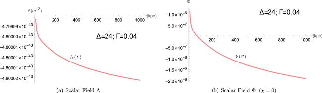
As an example, we now show that the spherically symmetric static vacuum solution of GWT obtained in the last section can be used to fit the experimental data of the rotation curve outside the Milky Way's stellar disk. Let the total mass M⊚ of all real matters within the edge of the Milky Way's stellar disk, the dimensional parameter d and the distance r be M⊚ = Δ × 1010M⊙, ∣d∣ = Γ × 10−20 m−1 and r = ϒ × 0.326 × 10²⁰ m respectively, where Δ, Γ and ϒ are undetermined dimensionless positive real parameters. By taking $\sqrt{\tfrac{{M}_{ \circledcirc }}{\kappa }}\approx \sqrt{{\rm{\Delta }}}\times 1.652\times {10}^{10}\,{{\rm{m}}}^{2}\cdot {{\rm{s}}}^{-2}$ [14], the rotation curve outside the Milky Way's stellar disk can be formulated through equation (45 ) as50 ) and (51 ) for GWT and GR respectively to fit the experimental data of the rotation velocity of stars whose distance r from the center of the Milky Way is greater than 13kpc, as shown in figure 1. It is clear that the rotation curve given by GWT can match the experimental data very well while that of GR cannot. The behavior of the scalar fields Λ(r) and Φ(r) determined by equations (48 ) and (49 ) respectively is plotted in figure 2 by setting M⊚ = 2.4 × 10¹¹M⊙ and ∣d∣ = 4 × 10⁻²² m−1.
$\begin{eqnarray}v({\rm{\Upsilon }})=100\sqrt{\displaystyle \frac{1.327}{0.326}\displaystyle \frac{{\rm{\Delta }}}{{\rm{\Upsilon }}}\displaystyle \frac{1}{\sqrt{{\left(0.326{\rm{\Gamma }}\right)}^{2}{{\rm{\Upsilon }}}^{2}+1}}-1.652\sqrt{{\rm{\Delta }}}\left[\displaystyle \frac{\mathrm{arsinh}(0.326{\rm{\Gamma }}{\rm{\Upsilon }})}{0.326{\rm{\Gamma }}{\rm{\Upsilon }}\sqrt{{\left(0.326{\rm{\Gamma }}\right)}^{2}{{\rm{\Upsilon }}}^{2}+1}}-1\right]}\quad \mathrm{km}\cdot {{\rm{s}}}^{-1}.\end{eqnarray}$
For comparison, the rotation curve given by GR with the same mass parameter reads [8, 14] $\begin{eqnarray}\tilde{v}({\rm{\Upsilon }})=100\sqrt{\displaystyle \frac{1.327}{0.326}\displaystyle \frac{{\rm{\Delta }}}{{\rm{\Upsilon }}}}\quad \mathrm{km}\cdot {{\rm{s}}}^{-1}.\end{eqnarray}$
Since the edge of the Milky Way's stellar disk is located at R⊚ = 13.9 ± 0.5 kpc [15], we use equations (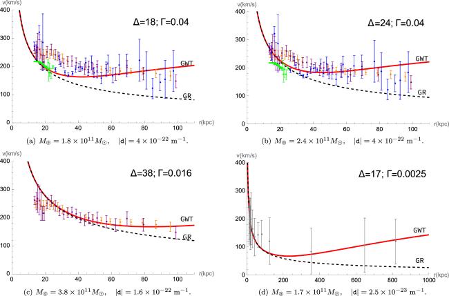
Figure 1. The rotation curves of GWT and GR in comparison with the observational data: The different experimental data with error bars of different colors are selected from references [16–19] and [20] respectively. The red solid line represents the theoretical curve of GWT, while the black dashed line represents the theoretical curve of GR. The parameters M⊚ and ∣d∣ take different values in figures 1 (a), (b), (c) and (d) respectively. |
Figure 2. The behaviors of the scalar fields Λ, (a), and Φ, (b), with respect to scale r. |
5. Conclusion and discussion
In this paper, a new GWT has been proposed based on Riemann–Cartan geometry. The geodesic deviation equation in Riemann–Cartan geometry is employed to infer the field equations and the property of torsion. The energy-momentum tensor of the matter fields in this geometry is also proposed. In comparison with GR, the GWT has more gravitational degrees of freedom characterized by torsion and two additional scalar fields, so that it is possible to explain the so-called DM and dark energy by gravitational effects.
To check this possibility, a spherically symmetric static vacuum solution of the GWT is obtained. It turns out that the solution does admit the asymptotic behavior of a galactic rotation curve. In particular, by suitably choosing the undetermined parameters, the solution can fit very well the experimental data of the rotation velocity of stars outside the Milky Way's stellar disk, while that of GR cannot. Hence, from the perspective of GWT, the galactic DM effect on the rotation curve is due to the additional gravitational degrees of freedom, including spacetime torsion. Therefore, the GWT proposed in this paper provides the example illustration that the so-called DM may just be a gravitational effect. Thus, one should consider going beyond GR at galactic or cosmological scales.
It should be noted that, unlike other alternative theories which explain the DM problem [4, 5], GWT inherits the basic idea of GR that gravity is the geometry of spacetime. Since the torsion field is coupled to the matter field, it is involved in the dynamical equation of the matter field. Therefore, in principle, one can distinguish GWT from other alternative theories by examining the characteristics of the dynamical evolution of the matter field, such as the formation of galactic nuclei and the internal structure of stars.
A few open issues for this new theory are listed below. First, a more realistic axisymmetric solution of the theory is desirable to confirm the resolution of the DM problem. Second, the scalar field Λ does not behave like a positive cosmological constant in the spherically symmetric static vacuum solution of the GWT obtained in section 3 . This reflects the fact that the solution is not suitable for a cosmological case. Hence, it is desirable to study the cosmological solution of GWT to check the issue of dark energy. Third, although the solution of GWT can explain the galactic rotation curve, to accept it as a tenable gravitational theory, one still needs to test the theory by other observations, such as gravitational waves, black hole images, and CMB, etc. Fourth, although the degrees of freedom on both sides of the field equations (17 ) and (18 ) coincide, a more careful analysis of the well-posedness of these equations is also important. We leave the above issues for further study.