


1. Introduction
Endofullerenes represent specialized structures within fullerene molecules, typically characterized by a spherical arrangement formed by carbon atoms, harboring different atoms or molecules within their interior. These structures often consist of atoms or molecules placed inside the fullerene shell, typically with an inner filling. Endofullerenes acquire unique properties due to the materials encapsulated within them [1, 2]. The inner filling significantly alters or enhances the electronic, magnetic, and chemical properties of endofullerenes. These properties enable diverse applications of endofullerenes, such as in nanotechnology, drug delivery, catalysis, and materials science [3–6]. These structures, by manipulating properties at the molecular level, could potentially play a significant role in various industrial fields in the future. Endofullerenes are complex exotic molecular structures that can be synthesized in different geometries, symbolized in terminology as X@Cn [7]. The synthesis of endofullerenes is typically achieved using two main methods: endohedral metallofullerenes, or endohedral complementary amines. However, our focus in the present work leans more towards endofullerenes containing hydrogen atoms. The synthesis of hydrogen-containing endofullerenes generally involves the interaction of hydrogen plasma with carbon structures. This process typically occurs under high temperature and pressure conditions. One method involves the reaction of carbon structures (usually graphite or carbon nanotubes) with hydrogen plasma, occurring within an environment where hydrogen gas is used to create a high-energy plasma. Carbon structures allow hydrogen atoms to interact within this plasma, enabling the incorporation of hydrogen into the carbon structures [8]. In this process, mechanisms such as the diffusion or absorption of hydrogen into carbon structures can play a role. This process facilitates the synthesis of hydrogen-containing endofullerenes by incorporating hydrogen into the carbon structures. The resulting structures can possess various properties, depending on the position and distribution of hydrogen within the endofullerene. Such hydrogen-containing endofullerenes have the potential to be used in various applications as hydrogen storage technologies and energy storage systems [9]. The properties and potential applications of endofullerenes stimulate in-depth investigations in this area and inspire new experimental/theoretical studies. Endofullerenes come in various types with different numbers of carbon atoms, exhibiting diverse geometric properties, such as their sizes and superficial features. By considering these differences, the Cn model is proposed in the present work to analyze characteristics such as the width, depth, thickness, and smoothing of endofullerenes. Theoretical studies on endofullerenes have predominantly focused on research areas such as the ionization potential, delocalizations, quantum information, photoionization, orbital distortion, and magnetic, optical, and thermal properties for the X@Cn complex [10–16].
Plasma is a state typically composed of ionized gases found at high temperatures and energy levels. However, it can also be easily generated under atmospheric conditions. In this case, electrons stripped from the outer shells of atoms create ions and free electrons, allowing positively and negatively charged particles to move freely. Plasma is best characterized by ionized gases and is typically formed in conditions of high temperature, high pressure, or high electric fields. It can be produced not only in natural settings, such as the Sun and stars, but also in laboratories and industries. The high-energy level determines the many characteristics of plasmas. Due to these properties, plasmas find applications in various areas, such as lasers, semiconductor manufacturing, materials processing, space research, nuclear fusion, and a wide array of atomic and molecular interactions [17]. Plasmas play a significant role in applications within atomic and molecular physics. Processes such as electron collisions with atoms, and absorption and emission of photons form the basis of plasma physics. These processes can also vary under the influence of magnetic fields, highlighting the complex nature of plasmas that need to be studied and controlled [18, 19]. In this manner, the interactions of plasmas at the atomic and molecular levels, processes such as energy transfer and conversion, constitute a significant research area in modern physics and technology. Studies in this area have the potential to lead to groundbreaking innovations in various fields, such as the production of new materials, space exploration, and energy generation [20]. The plasma environment provides optimal conditions for exciting an atom or molecule. However, within this excitation process, processes such as oscillator strengths, phase shifts, localizations of energy levels, and photoionization can be managed through the plasma shielding function. In this context, the H@Cn molecule is considered embedded within the plasma to experience a strong shielding effect in a quantum plasma. When modeling quantum plasma interactions, our work considers a more general exponential cosine screened Coulomb (MGECSC) potential. For more details about this potential, please refer to [21–23]. Plasma-encased endofullerene systems are a significant research subject for two reasons. Firstly, the plasma environment is highly functional in synthesizing or modifying endofullerenes. The high temperature and energy levels within plasma allow carbon structures to react in various ways. Under these conditions, carbon structures can form different molecular configurations under the influence of plasma. Alternatively, free atoms or molecules within the plasma can penetrate the interior of carbon structures and reside within endofullerenes. The formation of such endofullerenes is being investigated in fields such as materials science, nanotechnology, and plasma chemistry, exploring their potential applications. The second reason is that plasmas' shielding properties can be utilized to control certain spectral, electronic, optical, and spectroscopic characteristics of endofullerenes. The energy levels, oscillator strengths, mean excitation energy, photoionization dynamics, and static dipole polarizability of a hydrogen atom enclosed in an endohedral cage under the influence of a weak plasma interaction have been examined using a finite difference approach [24]. In the present work, the Cn model for endohedral confinement has been considered within the framework of the Woods–Saxon potential, taking into account the well depth V0, inner radius R0, thickness D, and smoothing parameter γ. This research distinctly elucidates the interaction between plasma and an endohedral molecule, suggesting that plasma plays an effective role in the physical properties of the aforementioned endohedral molecule. According to the overall findings of the study, there is strong competition between the effects of plasma interaction and the static endohedral cavity, thereby altering the electronic characteristics of the system. Motivated by the functionality provided by the plasma shielding effect, a similar study has been conducted in nonideal classical plasma [25], explaining the effects of a nonideal classical plasma environment on the photoionization dynamics of hydrogen-containing endofullerene molecules. In this study as well, significant features of both components of the plasma–endofullerene system have been identified.
The change in the aforementioned physical properties of the plasma–endofullerene system has been sufficiently motivating in the study of quantities such as the persistent current (PC) and induced magnetic field (IMF). In atoms, molecular systems, and artificially low-dimensional structures such as quantum dots, electric currents arising from atomic orbits and the associated induced magnetic fields are fundamentally linked to the movement of electrons. Electrons revolving around the atom's nucleus carry momentum due to their speed within their orbits, constituting moving charges that generate a current. Electrons orbiting in a loop correspondingly produce a magnetic field associated with that current, following Ampere's law of circulating currents around a moving charge. These orbital currents create magnetic fields at the atomic level, influencing the magnetic properties of atoms and molecules. Particularly, these effects may involve directing or altering magnetic moments, forming the basis for many magnetic materials and devices. The magnetic effects of orbital currents find applications in various fields, ranging from medical imaging devices, such as magnetic resonance imaging, to magnetic memories and sensors. The PC at the atomic level and the resultant IMF play a significant role in various aspects of modern technology, emphasizing the crucial importance of precise control over them [26–29]. Various physical factors may be involved in the formation and control of the PC and IMF in atomic systems. In this context, twisted lights have recently garnered attention because they involve the interaction between the orbital angular momentum and the spatial modes of the electromagnetic field. What makes twisted lights intriguing is their ability to alter significant steady currents, even in situations where there are no externally applied magnetic fields [30–32]. Such beams provide a significant advantage in that the dynamics of the laser–matter interaction do not depend on traditional selection rules, and the PC and IMF can then be generated simply by changing the orbital angular momentum index of the beam. It should be pointed out that an optical vortex has a significant effect on the charge current and magnetism in fullerene [31]. The Rashba spin–orbit interaction is a significant factor in the generation and modification of the PC and IMF due to the spin-twisting itinerant motion of electrons. It stabilizes the alternating motion of electrons by fixing their spins [32]. Another significant factor affecting the PC and IMF is the use of laser pulses. In this manner, time-delayed light pulses on nanoscopic and mesoscopic ring structures [33] and picosecond-shaped laser pulses on valley currents and magnetization in graphene rings [34, 35] establish a functional mechanism. Taking into account electron spin, the effectiveness of short intense circularly polarized π laser pulses on the PC and IMF of hydrogen atoms and certain ions has been thoroughly explained [36]. Several factors can have a significant impact on the PC and IMF in atomic systems. Exploring these factors not only guides experimental researchers, but also motivates theoretical studies to test new models and mechanisms. In this context, some effects, such as noncentral interactions, laser pulses, external magnetic fields, external electric fields, and spherical confinement, offer significant outcomes [37–40]. The common outcome of most of these studies is to elucidate how the PC and IMF can be modified by external influences. These explanations benefit the development of new opto-magnetic devices and magneto-optic materials, allowing the manipulation of many physical quantities that are sensitive to magnetic fields at the subatomic level. Endofullerenes can exhibit different magnetic properties, depending on the filling material inside them. This can be controlled by selecting the interior fillings or through external influences (such as external magnetic fields). Moreover, it can lay the groundwork for magnetic storage systems and spintronic applications. Endofullerenes could serve as potential building blocks for nanoscale electronic devices. These systems enable the control of nano-sized currents and magnetic fields. Research in these fields can be seen as significant steps toward understanding and controlling magnetic specifications of endofullerenes, and translating them into applications. This could lead to significant discoveries and advancements in materials science, nanotechnology, and magnetism fields. Considering the advantages of plasma in the synthesis of endofullerenes, as mentioned earlier, and the spectral properties that are modifiable by plasma's screening effects, the analysis of PC and IMF in plasma-encased endofullerene molecules is highly motivating.
The spins of electrons result in magnetic moments, influencing the formation of the PC and IMF in atomic systems. Spin is associated with the PC, and spin-carrying currents can have an impact on magnetic moments. Such currents play a significant role in the design of spintronic devices and magnetic storage systems [41]. On the other hand, the PC creates spin-circulation effects. This is when electrons rotate around their spin, parallel or antiparallel to charge currents. Spin–orbit coupling affects the electronic properties of the material and the behavior of carriers. Furthermore, in certain topological materials, there are connections between the spins and orbital motions of electrons [42]. For these reasons, the spin effects of charge currents are regarded as a significant area of research and application in fields such as materials science, magnetism, and spintronics. Therefore, this study will provide a relativistic examination by considering the spin effects within the Dirac formalism. The expectation from this study is to elucidate the effects of relativistic impacts and spin orientations on the PC and IMF covering plasma effects, endofullerene encapsulation, and spherical confinement. In doing so, experienced models and theoretical procedures will be utilized to parametrize these effects.
The study is organized as follows: in section 2 , the model and theoretical formalism are presented. Section 3 elucidates the obtained results. Section 4 is dedicated to a brief summary and conclusion of the work.
2. Theoretical model and procedure
For atomic systems exhibiting spherical symmetric interactions, the time-independent Dirac Hamiltonian in atomic units reads as8 ) is solved by employing the Runge–Kutta–Fehlberg method. For details, please refer to [52].
$\begin{eqnarray}{H}_{{\rm{D}}}=c{\boldsymbol{\alpha }}.{\boldsymbol{p}}+(\beta -I){c}^{2}+V(r),\end{eqnarray}$
where V(r) is the spherical symmetric potential, α and β are four-component matrices in standard Dirac–Pauli notation, I is a 4 × 4 unity matrix, and c is the light speed. Finding the eigenvalues and eigenvectors of the Dirac Hamiltonian to investigate relativistic effects is quite challenging due to its mathematical complexity. Additionally, the Dirac equation can be analytically solved for only a few potentials. To determine the eigenvalues and eigenvectors of the Dirac Hamiltonian with central potential, one must perform separation of the variables in the relevant Dirac equation, and this is where the real difficulty begins. The series of operations, considering the angular momentum ($\hat{J}$) and parity operator ($\hat{P}$) that commute with the Hamiltonian with respect to the center of the coordinate system, results in coupled differential equations for radial wave functions [43]. However, considering the separability of the Dirac equation, highly functional and well-established formalisms have been developed for obtaining two decoupled second-order differential equations in the analysis of the Dirac equation, such as the SUSY approach [44], and coupling the relativistic equation into large and small components by squaring the Dirac Hamiltonian [45, 46]. Within the modification of spin and angular variables, for an atomic system with the potential interaction V(r), the Dirac second-order equation in atomic units reads as follows [47–51] $\begin{eqnarray}\left[{\rm{\Upsilon }}{I}^{{\prime} }+\displaystyle \frac{1}{{r}^{2}}{\rm{\Delta }}\right]\left(\begin{array}{c}{G}_{\kappa }\\ {F}_{\kappa }\end{array}\right)=0,\end{eqnarray}$
with $\begin{eqnarray}{\rm{\Upsilon }}=-\displaystyle \frac{{{\rm{d}}}^{2}}{{\rm{d}}{r}^{2}}+\displaystyle \frac{{\kappa }^{2}}{{r}^{2}}+2(V(r)-E)-\displaystyle \frac{1}{{c}^{2}}{\left(V(r)-E\right)}^{2},\end{eqnarray}$
$\begin{eqnarray}{\rm{\Delta }}=\left(\begin{array}{cc}-\kappa & -\displaystyle \frac{{r}^{2}}{c}\displaystyle \frac{{\rm{d}}V(r)}{{\rm{d}}r}\\ \displaystyle \frac{{r}^{2}}{c}\displaystyle \frac{{\rm{d}}V(r)}{{\rm{d}}r} & \kappa \end{array}\right),\end{eqnarray}$
while E is the electron energy as the difference between the total and rest energy, and Gκ, Fκ are, respectively, the large and small component radial functions, ${I}^{{\prime} }$ is the 2 × 2 unit matrix. The relativistic momentum quantum number κ states are $\kappa =\mp (j+\tfrac{1}{2})$ and $j={\ell }\mp \tfrac{1}{2}$ in consideration of the orbital and total angular momentum quantum number ℓ and j, in which the mathematical formalism here works as κ = − ℓ for $j={\ell }-\tfrac{1}{2}$ and κ = ℓ + 1 for $j={\ell }+\tfrac{1}{2}$. The following nonunitary transformation matrix and r − independent when considering r2dV(r)/dr = η ≡ constant, is identified when considering Δ matrix elements $\begin{eqnarray}M=s\left(\begin{array}{cc}1 & -\displaystyle \frac{1}{c}\displaystyle \frac{\eta }{\kappa +{\rm{\Lambda }}}\\ -\displaystyle \frac{1}{c}\displaystyle \frac{\eta }{\kappa +{\rm{\Lambda }}} & 1\end{array}\right),\end{eqnarray}$
with s, which is a constant, and $\begin{eqnarray}{\rm{\Lambda }}=\kappa \sqrt{1-\displaystyle \frac{1}{{\kappa }^{2}{c}^{2}}{\left({r}^{2}\displaystyle \frac{{\rm{d}}V(r)}{{\rm{d}}r}\right)}^{2}}.\end{eqnarray}$
The relevant equations can be decoupled, by employing M and Λ, as well as the relation M−1ΔM $\begin{eqnarray}{M}^{-1}{\rm{\Delta }}M=\left(\begin{array}{cc}-{\rm{\Lambda }} & 0\\ 0 & {\rm{\Lambda }}\end{array}\right),\end{eqnarray}$
which, in turn, provides the following coupling form of the second-order Dirac equation $\begin{eqnarray}\left[{\rm{\Upsilon }}\pm \displaystyle \frac{{\rm{\Lambda }}}{{r}^{2}}\right]{F}_{\pm }(r)=0,\end{eqnarray}$
where F±(r) are scalar amplitudes. Equation (In a quantum plasma environment, an encapsulated H atom within a Cn fullerene is surrounded by a spherical encompassement with R0 radius. When a relativistic hydrogen atom is compressed to a spherical region with R0 radius under a pressure P, significant changes are observed in the atom's spectral energies. Therefore, studying the cases where the bound-state energy levels of the hydrogen atom change under such ultrarelativistic conditions is suitable for the ultrarelativistic condition and is important in understanding these situations. The pressure P referred to the case of when considering plasma-encased H@Cn under the spherical confinement1 ) is written as follows:
$\begin{eqnarray}P={\left(4\pi {R}_{0}^{3}\right)}^{-1}({E}_{0}-\langle V\rangle ),\end{eqnarray}$
where E0 is the ground state energy, and ⟨V⟩ is the estimated value of the potential energy. In this case, the spherical confinement potential reads $\begin{eqnarray}\begin{array}{l}{V}_{{\rm{c}}}(r)=\left\{\begin{array}{cc}0, & \mathrm{if}\,r\lt {R}_{0}\\ \infty , & \mathrm{if}\,r\geqslant {R}_{0}\end{array}\right..\end{array}\end{eqnarray}$
The Woods–Saxon potential model, which is one of the suitable models for static trapping hydrogen atoms within a fullerene that is compatible with experimental data, is considered [53]. Then, the static endohedral entrapping potential model is given by [54] $\begin{eqnarray}{V}_{\mathrm{EC}}(r)=\displaystyle \frac{{V}_{0}}{1+\exp (-\tfrac{r-({R}_{{\rm{c}}}+D)}{{\rm{\Gamma }}})}-\displaystyle \frac{{V}_{0}}{1+\exp (-\tfrac{r-{R}_{{\rm{c}}}}{{\rm{\Gamma }}})},\end{eqnarray}$
where V0 is the confinement strength, D is the spherical shell thickness, Rc is the inner radius of the endohedral cage, and Γ is the smoothing parameter. The strong screening effect of quantum plasma, complicated correlations in the plasma environment, and various perturbations can be most comprehensively modeled using the MGECSC potential [21, 23, 55]. This model is presented as follows: $\begin{eqnarray}{V}_{\mathrm{MGECSC}}(r)=-\displaystyle \frac{{{Ze}}^{2}}{4\pi {\varepsilon }_{0}r}(1+{br})\exp (-r/\lambda )\cos ({ar}/\lambda ),\end{eqnarray}$
where Z = 1 for the hydrogen atom, and a, b, and λ are the plasma shielding parameters. In such a scenario, by considering the combined effects of the spherical encompassement, quantum plasma, and endohedral trapping, the total interaction potential in equation ( $\begin{eqnarray}V(r)={V}_{\mathrm{MGECSC}}(r)+{V}_{\mathrm{EC}}(r)+{V}_{{\rm{c}}}(r).\end{eqnarray}$
Under these conditions, within the context of spherical symmetry motivation, the eigenvalue equation that needs to be solved is HD$\Psi$nκm(r, θ, φ) = E$\Psi$nκm(r, θ, φ), where $\Psi$nκm(r, θ, φ) is written, by considering large and small component radial functions, as $\begin{eqnarray}{{\rm{\Psi }}}_{n\kappa m}(r,\theta ,\varphi )=\left[\begin{array}{cc}{G}_{n\kappa }(r) & {\chi }_{\kappa m}(\theta ,\varphi )\\ {{\rm{i}}{F}}_{n\kappa }(r) & {\chi }_{-\kappa m}(\theta ,\varphi )\end{array}\right],\end{eqnarray}$
where χκm(θ, φ) is the spin angular function, expressed as $\begin{eqnarray}{\chi }_{\kappa m}(\theta ,\varphi )=\displaystyle \sum _{\sigma =\pm \tfrac{1}{2}}\lt {\ell }m-\sigma \displaystyle \frac{1}{2}\sigma | {\ell }\displaystyle \frac{1}{2}{jm}\gt {Y}_{{\ell }}^{m-\sigma }(\theta ,\varphi ){\phi }^{\sigma },\end{eqnarray}$
where $\lt {\ell }m-\sigma \tfrac{1}{2}\sigma | {\ell }\tfrac{1}{2}{jm}\gt $ are the Clebsch–Gordan coefficients, ${Y}_{{\ell }}^{m-\sigma }(\theta ,\varphi )$ are the spherical harmonics, and φσ is the spin functions as $\begin{eqnarray}{\phi }^{\tfrac{1}{2}}=\left(\begin{array}{c}1\\ 0\end{array}\right),{\phi }^{-\tfrac{1}{2}}=\left(\begin{array}{c}0\\ 1\end{array}\right),\end{eqnarray}$
and n, m are the principle quantum number and the projection of the angular quantum number j, on the z − axis, respectively.When considering the $\Psi$nκm(r, θ, φ) state, the probability current density is described as
$\begin{eqnarray}{\vec{J}}_{n\kappa m}(r,\theta ,\varphi )=\displaystyle \frac{{\rm{i}}{\hslash }}{2{m}_{e}}\left[{{\rm{\Psi }}}_{n\kappa m}{\boldsymbol{\nabla }}{{\rm{\Psi }}}_{n\kappa m}^{\star }-{{\rm{\Psi }}}_{n\kappa m}^{\star }{\boldsymbol{\nabla }}{{\rm{\Psi }}}_{n\kappa m}\right].\end{eqnarray}$
With e being the electron charge, the orbital charge currents and induced magnetic field are depicted in the following form $\begin{eqnarray}{I}_{n\kappa m}=-e{\int }_{0}^{\pi }{\int }_{0}^{{R}_{0}}r\vec{{J}_{n\kappa m}}(r,\theta ,\phi ){\rm{d}}r{\rm{d}}\theta {\rm{d}}\phi \vec{\phi },\quad \quad ({\rm{m}}\ne 0),\end{eqnarray}$
$\begin{eqnarray}{\vec{B}}_{n\kappa m}(\vec{r})=-\displaystyle \frac{{\mu }_{0}e}{4\pi }\int \displaystyle \frac{\vec{{J}_{n\kappa m}}(\vec{r})\times (\vec{r}-\vec{{r}^{{\prime} }})}{| \vec{r}-\vec{{r}^{{\prime} }}{| }^{3}}{{\rm{d}}}^{3}{r}^{{\prime} },\end{eqnarray}$
where μ0 is the vacuum permeability. For details, please refer to [56–58].3. Results and discussion
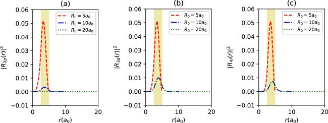
In this study, we analyze the charge-current generations (PC: I(mA)) and IMF (B(T)) of spherical confined quantum plasma-encased H@Cn within the framework of relativistic formalism. This analysis involves the effects of eight parameters: plasma shielding parameters (λ, b, and a), endofullerene static encompassement parameters (V0, D, Rc, and Γ), and the spherical confinement radius (R0). Additionally, the impact of spin orientations is examined. The methodology employed in the study has been tested by comparing its results with those of other studies under certain limits. In plasma environments modeled by the MGECSC potential for cases in the absence of endohedral encapsulation (V0 = 0) and without spherical confinement (R0 → 0), the relativistic bound-state energies of the embedded hydrogen atom has been compared with the results produced by the direct perturbation method [59]. A perfect agreement between the relativistic bound-state energies in all relevant tables in [59] for Z = 1 and our results has been observed. Additionally, when considering the b = 0 and b = a = 0 limits in the MGECSC potential, a very good agreement has been found between our relativistic results for the ECSC and SC potentials and the nonrelativistic results produced by the Ritz method [60] and the 1/N method [61]. These observed numerical agreements are important and motivating for testing the employed methodology. Figure 1 presents the interaction potential profiles given in equation (13 ). Except for the profile in panel-h, all synchronized wave functions in the other profiles are oriented towards spin up. As depicted in figure 1(a), the variation of λ in the range of 0−150a0 has a more pronounced effect in the weak regime of λ. An increase in λ in this weak regime makes the interaction potential more attractive. Table 1 shows the variation of the energy values of some quantum states synchronized with the parameter set of figure 1(a) as a function of λ. The attractiveness caused by λ in the interaction potential is also reflected in the localization of bound-state energies. As expected, an increase in λ in weak regimes significantly reduces the localization of bound states, followed by a subsequent stability in later increments of λ (See table 1). The dynamics of bound-state localizations are the primary factors influencing the PC (I) and IMF (B). Figure 2 depicts the variation of the PC and IMF as a function of λ. As seen in figure 2, an increase in λ within the range of 0−30a0 initially leads to a noticeable decrease in the PC and IMF, followed by a subsequent stabilization. Figure 3 is synchronized with figure 2 and shows the radial density probabilities (RDP) of 2p, 3d, and 4f states for three different values of λ. Due to the intensified interaction potential as λ increases, the RDP of bound states decreases, leading to a decrease in I and B (see figure 3). The most pronounced response to the λ change is observed in the 2p state, resulting in the most dynamic effects in the I−B characteristics within the 2p state.
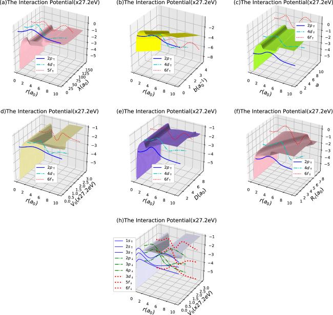
Figure 1. The interaction potential as the plasma plus endofullerene cage confinement and the relevant localized 2p − , 4d − , 6f − wave functions for: (a) b = 1/a0, a = 1, V0 = 20 eV, D = 3.5a0, Rc = 2.5a0, Γ = 0.1a0, and R0 = 10a0 as a function of r and λ; (b) λ = 80a0, a = 1, V0 = 20 eV, D = 3.5a0, Rc = 2.5a0, Γ = 0.1a0, and R0 = 10a0 as a function of r and b; (c) λ = 80a0, b = 1/a0, V0 = 20 eV, D = 3.5a0, Rc = 2.5a0, Γ = 0.1a0, and R0 = 10a0 as a function of r and a; (d) λ = 80a0, b = 1/a0, a = 1, D = 3.5a0, Rc = 2.5a0, Γ = 0.1a0, and R0 = 10a0 as a function of r and V0; (e) λ = 80a0, b = 1/a0, a = 1, V0 = 20 eV, Rc = 2.5a0, Γ = 0.1a0, and R0 = 10a0 as a function of r and D; (f) λ = 80a0, b = 1/a0, a = 1, V0 = 20 eV, D = 3.5a0, Γ = 0.1a0, and R0 = 10a0 as a function of r and Rc; (g) λ = 80a0, b = 1/a0, a = 1, V0 = 20 eV, D = 3.5a0, Rc = 2.5a0, and R0 = 10a0 as a function of r and Γ; (h) λ = 80a0, b = 1/a0, a = 1, D = 3.5a0, Rc = 2.5a0, and R0 = 10a0 as a function of r and V0, with some of the relevant s−, p−, d−, and f− wave functions with spin down. |
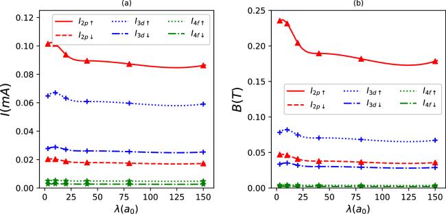
Figure 2. Persistent currents (a) and induced magnetic fields (b) as a function of λ for some quantum states in synchronization with the parameter set in figure 1(a). |
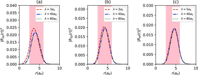
Figure 3. The radial density probabilities of 2p (a), 3d (b) and 4f states (c) with spin up for different λ values in synchronization with the parameter set in figure 2, as a function of r. The colored regions are the endohedral cage locations. |
Table 1. Energy values for the λ-change variations of some quantum states in synchronization with the parameter set in figure 1(a). |
| λ(a0) | ||||||
|---|---|---|---|---|---|---|
| Energy (eV) | 3 | 10 | 20 | 30 | 50 | 100 |
| −E1s | 23.369 184 | 38.704 208 | 43.723 837 | 45.616 53 | 47.205 723 | 48.437 189 |
| −E2p↑ | 16.129 887 | 34.313 389 | 40.400 069 | 42.591 642 | 44.394 841 | 45.771 928 |
| −E2p↓ | 16.131 188 | 34.314 721 | 40.401 542 | 42.593 187 | 44.396 454 | 45.773 599 |
| −E3d↑ | 11.740 014 | 29.964 451 | 36.399 876 | 38.722 676 | 40.633 287 | 42.091 242 |
| −E3d↓ | 11.741 007 | 29.965 421 | 36.400 953 | 38.723 804 | 40.634 461 | 42.092 453 |
| −E4f↑ | 6.663 161 | 24.726 202 | 31.475 002 | 33.922 509 | 35.937 320 | 37.474 900 |
| −E4f↓ | 6.664 184 | 24.727 182 | 31.476 073 | 33.923 620 | 35.938 475 | 37.476 074 |
| −E5g↑ | 18.855 542 | 25.889 311 | 28.455 147 | 30.570 619 | 32.186 171 | |
| −E5g↓ | 18.856 632 | 25.890 469 | 28.456 333 | 30.571 829 | 32.187 398 | |
Figure 1(b) depicts the interaction potential profile as a function of the plasma shielding parameter b and radial variable r. As observed, an increase in b enhances the attractiveness of the interaction potential, stabilizing the system concerning bound states. Table 2 illustrates the energy values of certain quantum states for the variation of b within 0 − 2.5/a0, when considering spin orientations. An increase in b leads to a more attractive interaction potential, resulting in a noticeable decrease in the localization of bound states. However, while the increase in the b parameter produces significant outcomes on energy levels, its effect on the PC and IMF is weak (See figure 4). Apart from the 2p level, the influence of b on the PC and IMF is quite uncertain in other states. Nevertheless, there is a remarkable effect of spin orientation on the values of I and B. Even though b has a strong impact on localizations, its weak effect on the I−B characteristics is somewhat unusual. However, as seen in figure 5(a), an increase in b mildly enhances the RDP of 2p, consequently leading to a slight increase in the PC and IMF for the 2p level. Similar elucidations hold true for the 3d and 4f states as well.
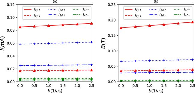
Figure 4. Persistent currents (a) and induced magnetic fields (b) as a function of b for some quantum states in synchronization with the parameter set in figure 1(b). |
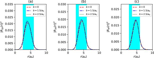
Figure 5. The radial density probabilities of 2p (a), 3d (b) and 4f states (c) with spin up for different b values in synchronization with the parameter set in figure 4, as a function of r. The colored regions are the endohedral cage locations. |
Table 2. Energy values for the b-change of some quantum states in synchronization with the parameter set in figure 1(b). |
| $b({a}_{0}^{-1})$ | ||||||
|---|---|---|---|---|---|---|
| Energy (eV) | 0 | 0.5 | 1 | 1.5 | 2 | 2.5 |
| −E1s | 22.135 896 | 35.126 214 | 48.126 379 | 61.136 746 | 74.157 680 | 87.189 554 |
| −E2p↑ | 19.603 685 | 32.512 469 | 45.425 905 | 58.343 962 | 71.266 607 | 84.193 810 |
| −E2p↓ | 19.605 418 | 32.514 162 | 45.427 561 | 58.345 581 | 71.268 193 | 84.195 362 |
| −E3d↑ | 16.003 262 | 28.862 127 | 41.725 028 | 54.591 926 | 67.462 782 | 80.337 562 |
| −E3d↓ | 16.004 513 | 28.863 354 | 41.726 230 | 54.593 104 | 67.463 937 | 80.338 695 |
| −E4f↑ | 11.466 867 | 24.275 925 | 37.088 719 | 49.905 199 | 62.725 317 | 75.549 028 |
| −E4f↓ | 11.468 070 | 24.277 109 | 37.089 886 | 49.906 348 | 62.726 448 | 75.550 143 |
| −E5g↑ | 6.257 403 | 19.016 984 | 31.780 344 | 44.547 389 | 57.318 036 | 70.092 208 |
| −E5g↓ | 6.258 648 | 19.018 218 | 31.781 567 | 44.548 601 | 57.319 236 | 70.093 397 |
Figure 1(c) explains the effects of the plasma parameter a on the interaction potential. In this quantum system encompassed within a spherical region of radius R0, there are no observable oscillations due to the a parameter, resulting in a weak repulsion. This weak repulsion leads to a decrease in the strength of the interaction potential, causing an inclination towards increased localization of bound states (See table 3). The weak impact of a on energy levels is reflected in the PC and IMF, as depicted in figure 6. An increase in a, most notably in the 2p state, causes a slight increase in the PC and IMF in other quantum states as well. This is because the RDP of 2p, 3d, and 4f states mildly increases as a increases (see figure 7). While the spin orientation does not alter the general character of I and B, there is a notable difference between up and down states, consistent with other findings. Figure 1(d) elucidates the variation in the interaction potential as a result that the depth of the endohedral cage increases. It is evident that as V0 increases, the encompassing effect of the interaction potential also rises. Consequently, a decrease in the energy levels of all bound states is expected, which is distinctly confirmed in table 4. The outcomes derived from the 2p level in the I−B characteristics differ from those originating from 3d and 4f. As the strength of the endohedral capsulation increases, there is a tendency for I2p and B2p to decrease while the others tend to increase, except for a slight initial increase (see figure 8). A more detailed analysis is needed to understand the reason behind this pattern. In figure 9, the RDP for 2p, 3d, and 4f are shown for cases without endohedral capsulation and for V0 = 20 eV and V0 = 80 eV. With regard to the 2p state, the electron's RDP not only moves away from the orbital center (r = 0) but also increases in a more stable manner. While $\vec{J}$ is the primary factor for persistent currents, it alone is not sufficient. As the electron localizes farther from the orbital center, the PC decreases. In this regard, for the 2p state, it could be said that the influence of the electron moving away from the orbital center on the I−B characteristics is more dominant compared to the increase in the RDP. For I3d and B3d, as the strength of the endohedral cage increases, the electron moves closer to the orbital center and the RDP increases. This leads to a significant increase in both the PC and IMF. This increase results in the same outcome for 4f as well. However, for quantum levels such as 4f, which are farther from the orbital center, the change in the PC and IMF is not clearly visible due to the scale of the graph in figure 8.
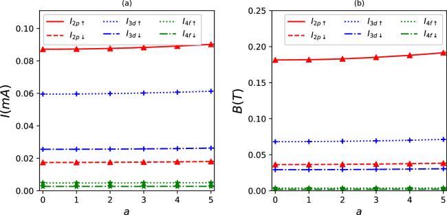
Figure 6. Persistent currents (a) and induced magnetic fields (b) as a function of a for some quantum states in synchronization with the parameter set in figure 1(c). |
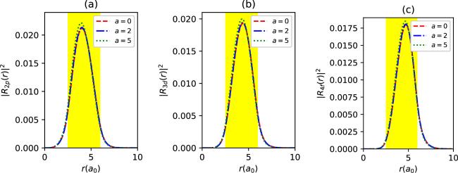
Figure 7. The radial density probabilities of 2p (a), 3d (b) and 4f states (c) with spin up for different a values in synchronization with the parameter set in figure 6, as a function of r. The colored regions are the endohedral cage locations. |
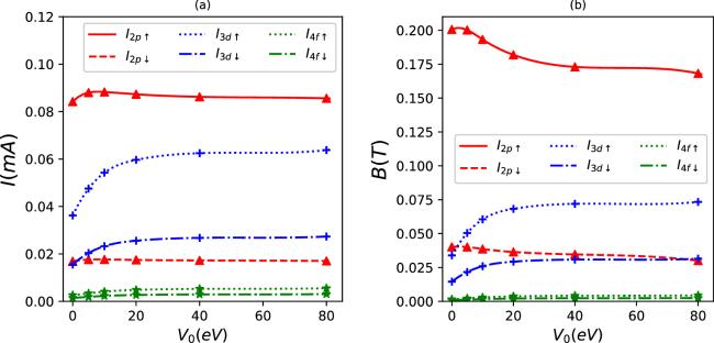
Figure 8. Persistent currents (a) and induced magnetic fields (b) as a function of V0 for some quantum states in synchronization with the parameter set in figure 1(d). |
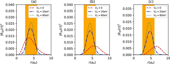
Figure 9. The radial density probabilities of 2p (a), 3d (b) and 4f states (c) with spin up for different V0 values in synchronization with the parameter set in figure 8, as a function of r. The colored regions are the endohedral cage locations. |
Table 3. Energy values for the a-change of some quantum states in synchronization with the parameter set in figure 1(c). |
| a | ||||||
|---|---|---|---|---|---|---|
| Energy (eV) | 0 | 1 | 2 | 3 | 4 | 5 |
| −E1s | 48.162 304 9 | 48.126 379 | 48.019 211 | 47.842 604 | 47.599 517 | 47.293 989 |
| −E2p↑ | 45.469 877 | 45.425 905 | 45.294 458 | 45.076 916 | 44.775 521 | 44.393 286 |
| −E2p↓ | 45.471 536 | 45.427 561 | 45.296 102 | 45.078 542 | 44.777 123 | 44.394 858 |
| −E3d↑ | 41.774 405 | 41.725 028 | 41.577 395 | 41.332 970 | 40.994 129 | 40.564 061 |
| −E3d↓ | 41.775 609 | 41.726 230 | 41.578 589 | 41.334 152 | 40.995 293 | 40.565 205 |
| −E4f↑ | 37.143 814 | 37.088 719 | 36.923 983 | 36.651 231 | 36.273 084 | 35.793 054 |
| −E4f↓ | 37.144 983 | 37.089 886 | 36.925 144 | 36.652 382 | 36.274 222 | 35.794 176 |
| −E5g↑ | 31.841 425 | 31.780 344 | 31.597 747 | 31.295 528 | 30.876 724 | 30.345 358 |
| −E5g↓ | 31.842 649 | 31.781 567 | 31.598 966 | 31.296 741 | 30.877 929 | 30.346 552 |
Table 4. Energy values for the V0-change of some quantum states in synchronization with the parameter set in figure 1(d). |
| V0(eV) | ||||||
|---|---|---|---|---|---|---|
| Energy (eV) | 0 | 5 | 10 | 20 | 30 | 40 |
| −E1s | 39.988 977 | 40.738 897 | 42.077 558 | 48.126 379 | 56.787 282 | 66.069 451 |
| −E2p↑ | 28.700 219 | 32.469 805 | 36.592 022 | 45.425 905 | 54.672 085 | 64.130 105 |
| −E2p↓ | 28.700 297 | 32.469 996 | 36.592 550 | 45.427 561 | 54.675 328 | 64.135 591 |
| −E3d↑ | 25.137 047 | 28.615 772 | 32.748 726 | 41.725 028 | 51.077 797 | 60.604 703 |
| −E3d↓ | 25.137 069 | 28.615 940 | 32.749 172 | 41.726 230 | 51.079 928 | 60.607 893 |
| −E4f↑ | 22.291 786 | 24.868 145 | 28.480 711 | 37.088 719 | 46.336 573 | 55.825 394 |
| −E4f↓ | 22.291 799 | 24.868 300 | 28.481 158 | 37.089 886 | 46.338 548 | 55.828 241 |
| −E5g↑ | 19.415 901 | 21.146 414 | 23.954 580 | 31.780 344 | 40.733 353 | 50.075 335 |
| −E5g↓ | 19.415 911 | 21.146 541 | 23.955 015 | 31.781 567 | 40.735 403 | 50.078 240 |
Figure 1(e) illustrates the confinement effect of the interaction potential as a function of the endohedral enclosure width (D) and the radial variable (r). The increase in D yields significant outcomes on quantum levels. The impact of the endohedral capsulation width on the localizations of quantum levels is demonstrated in table 5. It is observed that as the endohedral cage width increases, energy levels decrease, leading the system towards greater stability. Figure 10 illustrates the PC and IMF responses originating from the 2p, 3d, and 4f levels for spin up and spin down orientations concerning the increase in the endohedral fullerene width D. As observed, there is a significant decrease in the I−B characteristics due to the increase in the endohedral fullerene width D. Figure 11 shows the RDP of 2p, 3d, and 4f as a function of r for increasing values of the endohedral fullerene width D. An increase in the endohedral fullerene width results in the electron localizing over a wider area, which is expected to cause a decrease in the RDP. Additionally, the electron moves radially away from the center, supporting the decrease in the PC and IMF due to the diminishing RDP, ultimately leading to the prominent I−B characteristics observed in figure 10.
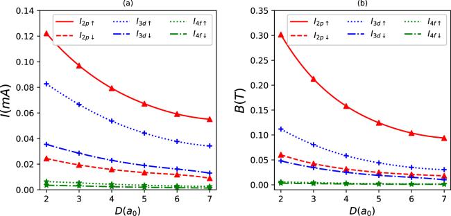
Figure 10. Persistent currents (a) and induced magnetic fields (b) as a function of D for some quantum states in synchronization with the parameter set in figure 1(e). |
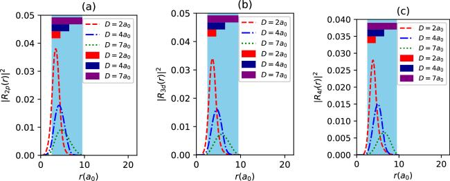
Figure 11. The radial density probabilities of 2p (a), 3d (b) and 4f states (c) with spin up for different D values in synchronization with the parameter set in figure 10, as a function of r. The colored regions are the endohedral cage locations. |
Table 5. Energy values for the D-change of some quantum states in synchronization with the parameter set in figure 1(e). |
| D(a0) | ||||||
|---|---|---|---|---|---|---|
| Energy (eV) | 2.5 | 3 | 3.5 | 4 | 5 | 6 |
| −E1s | 46.921 265 | 47.627 100 | 48.126 379 | 48.474 227 | 48.877 592 | 49.059 312 |
| −E2p↑ | 43.371 295 | 44.577 101 | 45.425 905 | 46.027 627 | 46.763 044 | 47.132 761 |
| −E2p↓ | 43.373 663 | 44.579 078 | 45.427 561 | 46.029 019 | 46.764 042 | 47.133 480 |
| −E3d↑ | 38.786 692 | 40.478 537 | 41.725 028 | 42.653 036 | 43.878 439 | 44.574 271 |
| −E3d↓ | 38.788 304 | 40.479 927 | 41.726 230 | 42.654 078 | 43.879 225 | 44.574 829 |
| −E4f↑ | 32.999 393 | 35.305 532 | 37.088 719 | 38.475 516 | 40.419 585 | 41.617 762 |
| −E4f↓ | 33.000 807 | 35.306 821 | 37.089 886 | 38.476 571 | 40.420 444 | 41.618 414 |
| −E5g↑ | 26.419 586 | 29.370 098 | 31.780 344 | 33.724 784 | 36.562 074 | 38.392 075 |
| −E5g↓ | 26.420 898 | 29.371 389 | 31.781 567 | 33.725 928 | 36.563 055 | 38.392 846 |
Figure 1(f) depicts the variation in the interaction potential as function of the inner radius of the endohedral cage (Rc) and the radial variable (r). Table 6 presents the energy values of certain quantum levels, including spin up and spin down orientations. The change in Rc forms a repulsive potential characteristic for the 1s and 2p energy levels, an attractive characteristic for 4f and 5g, and an initially attractive (Rc ≃ 3a0) and then repulsive characteristic for 3d. Figure 12 illustrates the behavior of the PC and IMF as a function of Rc. Although an increase in Rc creates an unstable response in the localization of certain energy levels, it causes a stable impact on the PC and IMF. The increase in the inner radius of the endohedral cage significantly decreases the PC and IMF (see figure 12). Figure 13 explains the behavior of the RDP of 2p, 3d, and 4f as a function of the radial variable (r) for different locations of the endohedral cage along the radial axis or, specifically, for an increasing inner radius. As observed, as the inner radius increases, both the electron's RDP decreases and it moves away from the radial center. These two outcomes, having a diminishing effect on the PC and IMF, complement each other, ultimately resulting in a notably decreasing I−B characteristic. Figure 1(g) explains the response due to the smoothing effect of the endohedral fullerene capsulation. As observed, as the smoothing increases, the interaction potential gains a repulsive characteristic, leading to a stable trend in terms of the localization of bound states. Table 7 illustrates the changes in the energy levels of quantum states due to smoothing. It is observed that as Γ increases, the endohedral fullerene capsulation exhibits a more unstable confining tendency, consequently resulting in a decrease in bound-state energies. However, this decrease is not very pronounced but rather follows a monotonic form. This monotonicity is also reflected in the PC and IMF characteristics (see figure 14). In a more repulsive potential, the probabilities of bound-state localizations are weaker. As depicted in figure 15, as Γ increases, the RDPs of 2p, 3d, and 4f show a slight decrease, which equally affects the PC and IMF characteristics (see figure 15). Table 8 presents the energies of certain quantum levels, depending on the increase in the spherical confinement effect (R0). As observed, the effective range of the spherical confinement concerning the energy levels of bound states is approximately 0−9a0. As R0 increases, the quantum levels decrease. However, outside this effective range, there is almost no change in energy levels. Figure 16 demonstrates the changes in the PC and IMF as a function of the spherical confinement effect. It is evident that as the spherical confinement range decreases, the electron's RDP decreases significantly. This decrease results in very clear reductions in the PC and IMF within the effective range of R0 (see figure 17).
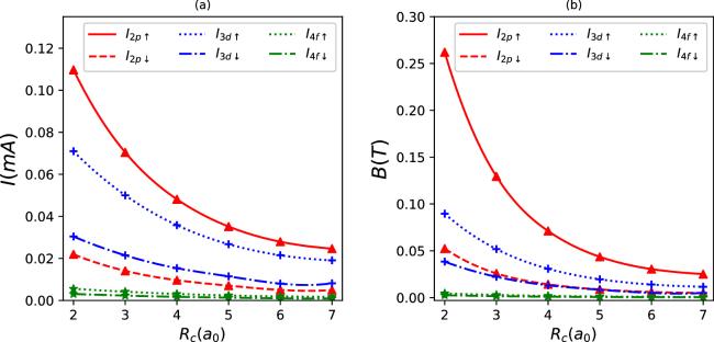
Figure 12. Persistent currents (a) and induced magnetic fields (b) as a function of Rc for some quantum states in synchronization with the parameter set in figure 1(f). |
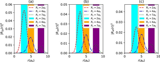
Figure 13. The radial density probabilities of 2p (a), 3d (b) and 4f states (c) with spin up for different Rc values in synchronization with the parameter set in figure 12, as a function of r. The colored regions are the endohedral cage locations. |
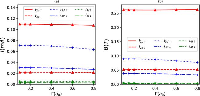
Figure 14. Persistent currents (a) and induced magnetic fields (b) as a function of Γ for some quantum states in synchronization with the parameter set in figure 1g. |
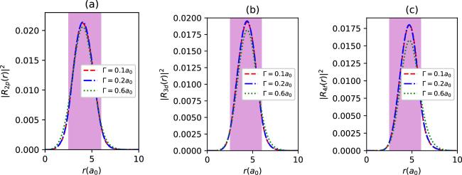
Figure 15. The radial density probabilities of 2p (a), 3d (b) and 4f states (c) with spin up for different Γ values in synchronization with the parameter set in figure 14, as a function of r. The colored regions are the endohedral cage locations. |
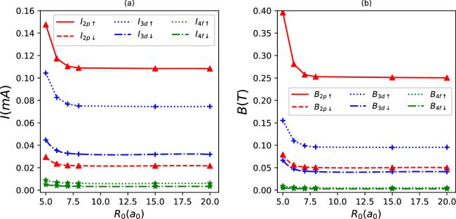
Figure 16. Persistent currents (a) and induced magnetic fields (b) as a function of R0 for some quantum states, when λ = 80a0, b = 1/a0, a = 1, V0 = 20 eV, D = 2.5a0, Rc = 2.5a0, and Γ = 0.1a0. |
Figure 17. The radial density probabilities of 2p (a), 3d (b) and 4f states (c) with spin up for different Γ values, when λ = 80a0, b = 1/a0, a = 1, V0 = 20 eV, D = 2.5a0, Rc = 2.5a0, and Γ = 0.1a0, as a function of r. The colored regions are the endohedral cage locations. |
Table 6. Energy values for the Rc-change of some quantum states in synchronization with the parameter set in figure 1(f). |
| Rc(a0) | ||||||
|---|---|---|---|---|---|---|
| Energy (eV) | 2.5 | 3 | 3.5 | 4 | 4.5 | 5 |
| −E1s | 48.126 379 | 46.838 977 | 45.838 567 | 45.033 708 | 44.355 463 | 43.738 906 |
| −E2p↑ | 45.425 905 | 44.919 674 | 44.420 278 | 43.944 126 | 43.487 505 | 43.024 168 |
| −E2p↓ | 45.427 561 | 44.921 733 | 44.422 819 | 43.947 226 | 43.491 244 | 43.028 630 |
| −E3d↑ | 41.725 028 | 41.996 429 | 42.073 720 | 42.026 291 | 41.891 154 | 41.670 046 |
| −E3d↓ | 41.726 230 | 41.997 772 | 42.075 257 | 42.028 064 | 41.893 186 | 41.672 316 |
| −E4f↑ | 37.088 719 | 38.146 105 | 38.867 048 | 39.335 035 | 39.608 013 | 39.706 681 |
| −E4f↓ | 37.089 886 | 38.147 304 | 38.868 326 | 39.336 431 | 39.609 549 | 39.708 341 |
| −E5g↑ | 31.780 344 | 33.581 400 | 34.955 272 | 35.978 111 | 36.711 330 | 37.183 243 |
| −E5g↓ | 31.781 567 | 33.582 605 | 34.956 491 | 35.979 376 | 36.712 661 | 37.184 626 |
Table 7. Energy values for the Γ-change of some quantum states in synchronization with the parameter set in figure 1(g). |
| Γ(a0) | ||||||
|---|---|---|---|---|---|---|
| Energy (eV) | 0.1 | 0.2 | 0.3 | 0.4 | 0.5 | 0.6 |
| −E1s | 48.126 379 | 47.881 460 | 47.547 542 | 47.182 011 | 46.841 177 | 46.566 542 |
| −E2p↑ | 45.425 905 | 45.108 175 | 44.630 063 | 44.033 354 | 43.365 404 | 42.670 114 |
| −E2p↓ | 45.427 561 | 45.109 029 | 44.630 672 | 44.033 843 | 43.365 810 | 42.670 450 |
| −E3d↑ | 41.725 028 | 41.406 715 | 40.919 619 | 40.304 372 | 39.610 619 | 38.885 777 |
| −E3d↓ | 41.726 230 | 41.407 357 | 40.920 084 | 40.304 751 | 39.610 940 | 38.886 051 |
| −E4f↑ | 37.088 719 | 36.777 899 | 36.309 170 | 35.724 994 | 35.075 309 | 34.406 898 |
| −E4f↓ | 37.089 886 | 36.778 524 | 36.309 622 | 35.725 361 | 35.075 619 | 34.407 164 |
| −E5g↑ | 31.780 344 | 31.478 579 | 31.046 868 | 30.532 894 | 29.983 593 | 29.439 173 |
| −E5g↓ | 31.781 567 | 31.479 231 | 31.047 334 | 30.533 267 | 29.983 905 | 29.439 438 |
Table 8. Energy values for the R0-change of some quantum states when λ = 80a0, b = 1/a0, a = 1, V0 = 20 eV, D = 3.5a0, Rc = 2.5a0, and Γ = 0.1a0. |
| R0(a0) | ||||||
|---|---|---|---|---|---|---|
| Energy (eV) | 3 | 5 | 9 | 11 | 15 | 20 |
| −E1s | 38.324 953 | 45.126 285 | 48.125 575 | 48.126 444 | 48.126 450 | 48.126 450 |
| −E2p↑ | 14.405 374 | 39.832 223 | 45.423 953 | 45.426 087 | 45.426 105 | 45.426 105 |
| −E2p↓ | 14.406 259 | 39.833 028 | 45.425 606 | 45.427 743 | 45.427 761 | 45.427 761 |
| −E3d↑ | − | 33.705 014 | 41.720 405 | 41.725 555 | 41.725 620 | 41.725 620 |
| −E3d↓ | − | 33.705 372 | 41.721 605 | 41.726 757 | 41.726 823 | 41.726 823 |
| −E4f↑ | − | 25.768 276 | 37.076 815 | 37.090 487 | 37.090 787 | 37.090 787 |
| −E4f↓ | − | 25.768 464 | 37.077 979 | 37.091 654 | 37.091 954 | 37.091 954 |
| −E5g↑ | − | 16.168 733 | 31.748 698 | 31.786 902 | 31.788 620 | 31.788 623 |
| −E5g↓ | − | 16.168 836 | 31.749 918 | 31.788 125 | 31.789 842 | 31.789 845 |
Table 9 illustrates the effect of the increase in the magnetic quantum number (m) on the PC and IMF. As observed, this effect arising from spherical harmonics is weak because the interaction potential does not have angular dependence. An increase in the magnetic quantum number (m) leads to angular probability densities localizing more towards the xy-plane rather than the z-axis. Consequently, an increase in angular probability and, therefore, an increase in the PC and IMF could be expected. However, the current integration might not provide a stable response to the increase in m due to angular normalization coefficients and Clebsch–Gordan coefficients. Therefore, the results originating from some numerical cases might predominate in the increment of the angular probability when considering the PC and IMF. In summary, the study delves into the intricate interplay among different parameters affecting the PCs and IMFs of quantum plasma-encased endohedral fullerenes. The results show a nuanced dependence on these parameters, with certain regimes leading to enhanced or reduced PCs and magnetic fields. The interplay of plasma screening, endofullerene encapsulation, spherical confinement, and other factors adds a layer of complexity to the behavior of these quantum systems. The detailed analysis and presentation of results provide insights into the underlying physics and potential applications of such systems in quantum information processing and other fields.
Table 9. The magnetic quantum number (m) effect on the PC and IMF, when λ = 80a0, b = 1/a0, a = 1, V0 = 20 eV, D = 3.5a0, Rc = 2.5a0, Γ = 0.1a0, and R0 = 10a0. |
| ∣nℓmℓms⟩ | I(mA) | B(T) |
|---|---|---|
| ∣111 + 1/2⟩ | 0.087 317 | 0.181 876 |
| ∣111 − 1/2⟩ | 0.017 464 | 0.036 404 |
| ∣122 + 1/2⟩ | 0.019 171 | 0.043 876 |
| ∣122 − 1/2⟩ | 0.002 130 | 0.004 875 |
| ∣121 + 1/2⟩ | 0.059 643 | 0.068 252 |
| ∣121 − 1/2⟩ | 0.025 561 | 0.029 254 |
| ∣133 + 1/2⟩ | 0.000 115 | 0.000 263 |
| ∣133 − 1/2⟩ | 0.000 008 | 0.000 020 |
| ∣132 + 1/2⟩ | 0.005 802 | 0.008 795 |
| ∣132 − 1/2⟩ | 0.001 582 | 0.002 398 |
| ∣131 + 1/2⟩ | 0.004 809 | 0.003 645 |
| ∣131 − 1/2⟩ | 0.002 671 | 0.002 024 |
4. Concluding remarks
As expected, while spin orientations create a very subtle difference in bound-state energies, there is a noticeable difference between the PC and IMF of spin up and down configurations when considering every parameter change. The values of I−B for spin up configurations are consistently larger. The difference between the spin up and down states is most significant for the PC and IMF of quantum levels closer to the hydrogen nucleus, diminishing as one moves away from the nucleus towards outer levels. The impact of the λ parameter is more pronounced on both the energies and I−B in weaker regimes, approximately around λ ≃ 0−40a0. While the b screening parameter significantly affects bound-state energies, its effect on the PC and IMF is unexpectedly weak. Meanwhile, the a screening parameter has a weak effect on both the energies and the I−B characteristics. In terms of plasma functionality, the most effective and functional parameter for the PC and IMF is λ. This is advantageous from an experimental perspective as well because λ is a parameter that is dependent on plasma temperature T and plasma density n, allowing alterations in I−B characteristics with changes in n and T. An increase in the depth of endohedral fullerene encapsulation (V0) affects the PC and IMF of 2p and 3d−4f levels in different ways. In this context, it has become evident in the analysis of V0 that the I−B characteristic is not solely dependent on the current density ($\vec{J}$) but also on the electron's radial distance from the center. The effective range of V0 for the PC and IMF has been determined to be 0−30 eV under the given conditions. As the endohedral fullerene expands (D), both the RDP decreases and the electron moves away from the radial center. Consequently, an increase in D effectively reduces I−B values. The inner radius of the endofullerene (Rc) stands out as the most significant and functional parameter for the PC and IMF. In this regard, it could be an alternative to D. The effect of smoothing (Γ) effect should be considered as a fine-tuning parameter for the PC and IMF of endofullerenes. This is because smoothing requires less experimental effort and has a very weak impact on I−B characteristics. The spherical confinement (R0) also affects the PC and IMF. However, for the numerical values within the given parameter set, the functional range of R0 is approximately 0−10a0. Even without angular interactions, spherical harmonics influence the PC and IMF. However, the localization effect of ${Y}_{{\ell }}^{m}$ alone may not be the sole impactful factor in this influence.
Conflicts of interest/Competing interests
Mustafa Kemal Bahar is the only author of this study.