


1. Introduction
The utilization of mesoscopic superconducting circuits [1] has significantly propelled the advancement of cavity quantum electrodynamics (QED). In 2004, Wallraff et al demonstrated the coherent superposition of a single qubit and a single photon on a superconducting chip, thus pioneering the concept of circuit QED [2]. Subsequently, superconducting qubits leveraging the macroscopic quantum effects inherent in Josephson junctions [3] have found widespread application in quantum state engineering [4, 5], quantum information processing [6], and quantum computing [7–10].
In contrast to cavity QED, circuit QED systems featuring superconducting qubits exhibit stronger coupling to the on-chip cavity, frequent photon exchange, extended coherence times, heightened stability, and greater adaptability to solid-state environments [11]. The emergence of circuit QED has paved the way for in-depth exploration of the strong interaction between light and matter. In 2010, Niemczyk et al achieved the first experimental demonstration of ultrastrong coupling (USC) by interfacing a superconducting artificial atom with the on-chip cavity [12]. Subsequently, numerous theoretical analyses [13–15] and experimental validations [16–19] predicated on the USC system have proliferated.
In the USC regime, the contribution of interaction terms in the quantum Rabi model (QRM) is comparable to that of non-interaction terms [20]. As a result, the validity of the rotating wave approximation (RWA) and the Jaynes–Cummings (JC) model is compromised, necessitating the consideration of counter-rotating wave terms In this regime, the exchange of photons between the qubits and cavity occurs more frequently before coherence is lost, leading to the emergence of unique physical phenomena. For example, an unconventional photon blocking effect manifests in the driven cavity QED system [21]. Additionally, the rapid transfer of photons through coherent Rabi oscillations enables the realization of multi-photon Rabi oscillations, which holds significant implications for quantum state manipulation and the operation of atoms and photons inside the cavity [22].
Furthermore, the presence of counter-rotating wave terms led Garziano et al to predict the simultaneous excitation of two or more atoms by a single photon [23], a phenomenon subsequently verified by experiments [24]. Recent studies have demonstrated that one-photon-two-atom excitation processes can result in single- or two-photon blockade [25], two-color electromagnetically induced transparency [26], and spin squeezing in an ensemble of many two-level atoms [27]. Moreover, as the coupling strength increases, the eigenenergy spectrum of the USC system no longer maintains a clear delineation, but exhibits the hybridization of eigenstates at specific positions, leading to the phenomena of level crossing and avoided-crossing in the energy spectrum. These remarkable developments have piqued our research interest.
Non-Gaussian states have gained widespread utility as quantum resources in the domains of quantum computation and quantum communication [28]. In contrast to Gaussian states, non-Gaussian states demonstrate heightened non-classicality [29], making the non-Gaussian input state a pivotal element in quantum computing assurances [30]. The non-Gaussian characteristic of the output field can be discerned through the intensity-amplitude correlation [31–34].
In 2000, Carmichael et al introduced hθ(τ), which represents the correlation of intensity and field amplitude and establishes the link between the particle and wave nature of light [35]. The second-order fluctuations in the intensity-amplitude correlation signify the squeezing properties of the system. Given that the odd-order fluctuations of the Gaussian state are zero, the identification of the non-Gaussian feature is prompted when the output state demonstrates third-order fluctuations. The time asymmetry of third-order fluctuations in the intensity-amplitude correlation, observed through conditional homodyne detection (CHD), serves as an indicator of the breakdown of detailed balance and probes the non-Gaussian feature of the system [36]. Here, we leverage the third-order fluctuations in the intensity-amplitude correlation to identify the non-Gaussian feature of the output field from the double qubit-cavity ultrastrong coupling system, and anticipate the application of our system in the exploration of nonlinear optics [37].
This paper focuses on investigating the non-Gaussian characteristics of a double superconducting qubit-cavity coupling system in the ultrastrong coupling (USC) regime. As a result of the presence of counter-rotating wave terms in the quantum Rabi model (QRM), a splitting anti-crossing between levels three and four emerges in the eigenenergy spectrum. Notably, unlike the situation in weak coupling, two unconventional phenomena, namely, energy level crossing and avoided-crossing, manifest in the energy spectrum. In order to explore these phenomena, we designate the third excited state as the target state and align the frequency of the driving field with the transition from the ground state to the third excited state. This reduces the cavity quantum electrodynamics (QED) system to a four-level model driven by a light field with a Rabi frequency. Subsequently, we analyze the intensity-amplitude correlation of the output field from the circuit QED system.
It is crucial to underscore that in the USC regime, the annihilation (creation) operator in the standard input-output relations under the rotating wave approximation (RWA) necessitates modification. In comparison with our prior work based on atomic systems [38], we observe that the increase in the third-order term, representative of the non-Gaussian feature of the output light, leads to a more pronounced violation of classical inequalities in the intensity-amplitude correlation function of the circuit QED system under USC. This discovery highlights the potential of applying this system in the realms of nonlinear optics and the generation of non-classical states.
2. Model and system
We consider an ultrastrong coupling (USC) system composed of two superconducting qubits coupled to a single-mode cavity in the regime where the detuning between the cavity and the qubit, denoted as Δ = ωc − ωq, is significantly larger than their coupling rate g (ωc and ωq represent the resonance frequencies of the cavity mode and the qubit transition frequency). Furthermore, the cavity mode is is driven by a coherent laser field with frequency ωl and the driving strength ϵ. The Hamiltonian describing the circuit QED system is given by
$\begin{eqnarray}\begin{array}{l}{H}_{S}={H}_{0}+{H}_{d},\end{array}\end{eqnarray}$
where the Hamiltonian of the quantum Rabi model (ℏ = 1) is described by [23] $\begin{eqnarray}\begin{array}{l}{H}_{0}={\omega }_{c}{a}^{\dagger }a+\displaystyle \sum _{i}\left[\displaystyle \frac{{\omega }_{q}}{2}{\sigma }_{z}^{(i)}+{gX}\left(\cos \phi {\sigma }_{x}^{(i)}+\sin \phi {\sigma }_{z}^{(i)}\right)\right],\end{array}\end{eqnarray}$
and the interactive Hamiltonian between the driven field and the cavity mode can be expressed as [39] $\begin{eqnarray}\begin{array}{l}{H}_{d}=\varepsilon \cos ({\omega }_{l}t)X,\end{array}\end{eqnarray}$
where X = a + a†, a and a† are the annihilation and creation operators for cavity mode, ${\sigma }_{x}^{(i)}$ and ${\sigma }_{z}^{(i)}$ are Pauli operators for the ith qubit.In contrast to the Jaynes–Cummings model, the Hamiltonian in equation (2 ) explicitly includes four counter-rotating terms, rendering it challenging to derive exact analytical solutions of the Rabi model. In this study, we employ a convenient method to obtain highly accurate numerical solutions of the Rabi model employing an approach described in [21]. Specifically, we expand the Rabi Hamiltonian in a basis comprised of the eigenstates ∣$Psi$n⟩ of H0. Based on the eigenenergy spectrum presented in [40], we consider two scenarios of energy level crossing and avoided level crossing [g/ωq = 0.2, 0.7] for analysis.
In these scenarios, the system can be represented as a four-level model, and the Hamiltonian can be simplified as follows
$\begin{eqnarray}\begin{array}{l}{H}_{S}=\displaystyle \frac{{\rm{\Omega }}}{2}\ ({\sigma }_{03}+{\sigma }_{30}),\end{array}\end{eqnarray}$
where Ω = ϵ⟨$Psi$0∣(a + a†)∣$Psi$3⟩. Thus the modified master equation can be written as $\begin{eqnarray}\begin{array}{l}\dot{\rho }(t)=-{\rm{i}}[{H}_{s},\rho (t)]+{{ \mathcal L }}_{c}\rho (t)+\displaystyle \sum _{i=1,2}{{ \mathcal L }}_{a}^{(i)}\rho (t),\end{array}\end{eqnarray}$
where ${{ \mathcal L }}_{x}\rho (t)={\sum }_{j,k\gt j}{{\rm{\Gamma }}}_{x}^{{jk}}{ \mathcal D }[| {\psi }_{j}\rangle \langle {\psi }_{k}| ]\rho (t)$, for $x=c,{\sigma }_{-}^{(i)}$. The superoperator ${ \mathcal D }$ is defined as ${ \mathcal D }[O]\rho =\tfrac{1}{2}(2\,O\,\rho \,{O}^{\dagger }\,-\rho \,{O}^{\dagger }\,O-{O}^{\dagger }\,O\,\rho )$. The relaxation coefficients of the qubits and the cavity mode are defined as $\begin{eqnarray}\begin{array}{rcl}{{\rm{\Gamma }}}_{x}^{{jk}} & \equiv & {\gamma }_{i}\displaystyle \frac{{E}_{{kj}}}{{\omega }_{q}}| \langle {\psi }_{j}| ({\sigma }_{-}^{(i)}-{\sigma }_{+}^{(i)})| {\psi }_{k}\rangle {| }^{2},\,\,(x={\sigma }_{-}^{(i)}),\\ {{\rm{\Gamma }}}_{x}^{{jk}} & \equiv & \kappa \ \displaystyle \frac{{E}_{{kj}}}{{\omega }_{c}}| \langle {\psi }_{j}| (\ a-{a}^{\dagger }\ )| {\psi }_{k}\rangle {| }^{2},\,\,(x=c),\end{array}\end{eqnarray}$
where γi and κ are standard damping rates of the qubits and cavity, and we set γ1 = γ2 = γ in this paper. The eigenstates are labeled according to En > Em for n > m.Referring to the master equation in equation (5 ), we can derive the evolution equations for the density-matrix elements as follows
$\begin{eqnarray}\begin{array}{rcl}{\dot{\rho }}_{00} & = & {{\rm{\Gamma }}}_{10}{\rho }_{11}+{{\rm{\Gamma }}}_{20}{\rho }_{22}+{{\rm{\Gamma }}}_{30}{\rho }_{33}+\displaystyle \frac{{\rm{i}}\ {\rm{\Omega }}}{2}({\rho }_{03}-{\rho }_{30}),\\ {\dot{\rho }}_{11} & = & -{{\rm{\Gamma }}}_{10}{\rho }_{11}++{{\rm{\Gamma }}}_{21}{\rho }_{22}+{{\rm{\Gamma }}}_{31}{\rho }_{33},\\ {\dot{\rho }}_{33} & = & -\displaystyle \frac{{{\rm{\Gamma }}}_{30}+{{\rm{\Gamma }}}_{31}+{{\rm{\Gamma }}}_{32}}{2}{\rho }_{33}-\displaystyle \frac{{\rm{i}}\ {\rm{\Omega }}}{2}({\rho }_{03}-{\rho }_{30}),\\ {\dot{\rho }}_{03} & = & -\displaystyle \frac{{{\rm{\Gamma }}}_{30}+{{\rm{\Gamma }}}_{31}+{{\rm{\Gamma }}}_{32}}{2}{\rho }_{03}+\displaystyle \frac{{\rm{i}}\ {\rm{\Omega }}}{2}({\rho }_{00}-{\rho }_{33}),\\ {\dot{\rho }}_{01} & = & -\displaystyle \frac{{{\rm{\Gamma }}}_{10}}{2}{\rho }_{01}-\displaystyle \frac{{\rm{i}}\ {\rm{\Omega }}}{2}{\rho }_{31},\\ {\dot{\rho }}_{13} & = & -\displaystyle \frac{{{\rm{\Gamma }}}_{10}+{{\rm{\Gamma }}}_{30}+{{\rm{\Gamma }}}_{31}+{{\rm{\Gamma }}}_{32}}{2}{\rho }_{13}+\displaystyle \frac{{\rm{i}}\ {\rm{\Omega }}}{2}{\rho }_{10},\end{array}\end{eqnarray}$
with ρ22 = 1 − ρ00 − ρ11 − ρ33 and ${\rho }_{{ji}}={\left({\rho }_{{ij}}\right)}^{* }$ for $i,j\in \left\{1,2,3\right\}$. Correspondingly, we can derive the stationary solutions of the system as follows $\begin{eqnarray}\begin{array}{rcl}{\rho }_{00}^{{ss}} & = & \displaystyle \frac{{{\rm{\Gamma }}}_{10}({{\rm{\Gamma }}}_{20}+{{\rm{\Gamma }}}_{21})({A}^{2}+{{\rm{\Omega }}}^{2})}{{{\rm{\Gamma }}}_{10}({{\rm{\Gamma }}}_{20}+{{\rm{\Gamma }}}_{21}){A}^{2}+B\ {{\rm{\Omega }}}^{2}},\\ {\rho }_{11}^{{ss}} & = & \displaystyle \frac{\left[{{\rm{\Gamma }}}_{31}({{\rm{\Gamma }}}_{20}+{{\rm{\Gamma }}}_{21})+{{\rm{\Gamma }}}_{32}{{\rm{\Gamma }}}_{21}\right]{{\rm{\Omega }}}^{2}}{{{\rm{\Gamma }}}_{10}({{\rm{\Gamma }}}_{20}+{{\rm{\Gamma }}}_{21}){A}^{2}+B\ {{\rm{\Omega }}}^{2}},\\ {\rho }_{22}^{{ss}} & = & \displaystyle \frac{{{\rm{\Gamma }}}_{10}{{\rm{\Gamma }}}_{32}{{\rm{\Omega }}}^{2}}{{{\rm{\Gamma }}}_{10}({{\rm{\Gamma }}}_{20}+{{\rm{\Gamma }}}_{21}){A}^{2}+B\ {{\rm{\Omega }}}^{2}},\\ {\rho }_{33}^{{ss}} & = & \displaystyle \frac{{{\rm{\Gamma }}}_{10}({{\rm{\Gamma }}}_{20}+{{\rm{\Gamma }}}_{21}){{\rm{\Omega }}}^{2}}{{{\rm{\Gamma }}}_{10}({{\rm{\Gamma }}}_{20}+{{\rm{\Gamma }}}_{21}){A}^{2}+B\ {{\rm{\Omega }}}^{2}},\\ {\rho }_{03}^{{ss}} & = & \displaystyle \frac{i{{\rm{\Gamma }}}_{10}({{\rm{\Gamma }}}_{20}+{{\rm{\Gamma }}}_{21})A{\rm{\Omega }}}{{{\rm{\Gamma }}}_{10}({{\rm{\Gamma }}}_{20}+{{\rm{\Gamma }}}_{21}){A}^{2}+B\ {{\rm{\Omega }}}^{2}},\quad {\rho }_{01}^{{ss}}={\rho }_{13}^{{ss}}=0,\end{array}\end{eqnarray}$
where A = Γ30 + Γ31 + Γ32 and B = (2Γ10 + Γ31)(Γ20 + Γ21) + Γ32(Γ10 + Γ21).3. Non-Gaussian feature of the output field
The non-Gaussian feature of the light field can be revealed by third-order fluctuations in the intensity-amplitude correlation [36]. In the setup of conditional homodyne detection (CHD), the intensity-amplitude correlation is obtained by conducting balanced homodyne detection (BHD) of the quadrature amplitude ${E}_{\theta }\propto {\hat{a}}_{\theta }$ when the photon detector is triggered, and by measuring the intensity $I\propto {\hat{a}}^{\dagger }\hat{a}$ at the photon detector DI [33–35]. The measurement signal from CHD, denoted as ⟨:I(0)Eθ(τ):⟩, where “::” denotes the time and normal ordering. According to the input-output relations proposed by Ridolfo et al [41], the annihilation operator $\hat{a}$ in the weak coupling regime is replaced by the operator ${\dot{X}}^{+}$ in the case of strong coupling regime. Thus, the intensity-amplitude correlation function for the output field in normalized form is
$\begin{eqnarray}\begin{array}{l}{h}_{\theta }(\tau )=\displaystyle \frac{\langle :{\dot{X}}^{-}(0){\dot{X}}^{+}(0){\dot{X}}_{\theta }(\tau ):\rangle }{\langle {\dot{X}}^{-}{\dot{X}}^{+}\rangle \langle {\dot{X}}_{\theta }\rangle }.\end{array}\end{eqnarray}$
Here we defined the quadrature amplitude operator as $\begin{eqnarray}\begin{array}{l}{\dot{X}}_{\theta }=\displaystyle \frac{1}{2}({\dot{X}}^{+}{{\rm{e}}}^{-{\rm{i}}\theta }+{\dot{X}}^{-}{{\rm{e}}}^{{\rm{i}}\theta }),\end{array}\end{eqnarray}$
where θ is the phase difference between the local oscillator (LO) and the driving field which is adjusted to be π/2.In equation (10 ), ${\dot{X}}^{+}$ (${\dot{X}}^{-}$) represent the positive (negative) frequency components of $\dot{X}$, where $\dot{X}=-{\rm{i}}{X}_{0}(a-{a}^{\dagger })$. And X0 is the rms zero-point field amplitude which is assumed to be unit in this paper. By expanding $\dot{X}$ in the dressed state basis ∣$Psi$i⟩, ${\dot{X}}^{+}$ can be expressed as ${\dot{X}}^{+}=-{\rm{i}}{\sum }_{m,n\gt m}{E}_{{nm}}{X}_{{mn}}{\sigma }_{{mn}}$, where ${X}_{{mn}}=\langle {\psi }_{m}| \dot{X}| {\psi }_{n}\rangle $ and ${\dot{X}}^{-}={\left({\dot{X}}^{+}\right)}^{\dagger }$. For the four-level system, the expression can be derived as follows
$\begin{eqnarray}\begin{array}{l}{\dot{X}}^{+}(\tau )={\alpha }_{01}{\sigma }_{01}(\tau )+{\alpha }_{03}{\sigma }_{03}(\tau )+{\alpha }_{13}{\sigma }_{13}(\tau ),\end{array}\end{eqnarray}$
where αmn = −Enm⟨$Psi$m∣a − a†∣$Psi$n⟩.Splitting the field operator into the mean field and fluctuation, i.e., ${\dot{X}}^{+}=\langle {\dot{X}}^{+}\rangle +{\rm{\Delta }}{\dot{X}}^{+}$, allows the intensity-amplitude correlation function for the output field to be expressed as the sum of a squeezing term and an incoherent term
$\begin{eqnarray}\begin{array}{l}{h}_{\theta }(\tau )=1+{h}_{\theta }^{(2)}(\tau )+{h}_{\theta }^{(3)}(\tau ),\end{array}\end{eqnarray}$
where $\begin{eqnarray}{h}_{\theta }^{(2)}(\tau )=\displaystyle \frac{2\langle :{\rm{\Delta }}{\dot{X}}_{\theta }(0){\rm{\Delta }}{\dot{X}}_{\theta }(\tau ):\rangle }{\langle {\dot{X}}^{-}{\dot{X}}^{+}\rangle },\end{eqnarray}$
$\begin{eqnarray}{h}_{\theta }^{(3)}(\tau )=\displaystyle \frac{\langle :{\rm{\Delta }}{\dot{X}}^{-}(0){\rm{\Delta }}{\dot{X}}_{\theta }(\tau ){\rm{\Delta }}{\dot{X}}^{+}(0):\rangle }{\langle {\dot{X}}^{-}{\dot{X}}^{+}\rangle \langle {\dot{X}}_{\theta }\rangle }.\end{eqnarray}$
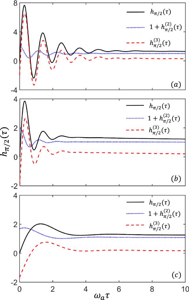
Figure 1. The numerical results for the intensity-amplitude correlation function hπ/2(τ) and its decomposition based on the order of fluctuations are presented for the following cases: (a) κ = 2, ϵ = 8; (b) κ = 4, ϵ = 8; and (c) κ = 2, ϵ = 2. The units are in terms of ωa, where ωa = 10−3ωq. We set γ = 0.01ωa, and the remaining parameters are g/ωq = 0.2, ωc/ωq = 1.915, and θ = π/6. |
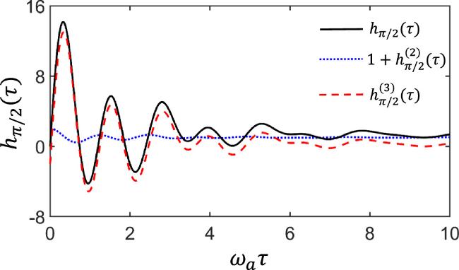
Figure 2. The numerical results for the intensity-amplitude correlation function hπ/2(τ) and its decomposition based on the order of fluctuations are provided for κ = 2, ϵ = 8 (measured in units of ωa, where ωa = 10−3ωq). All parameters are consistent with those in figure 1, except for g/ωq = 0.7. |
According to the classical inequality in [35]
$\begin{eqnarray}\begin{array}{l}| {h}_{\theta }(\tau )-1| \leqslant | {h}_{\theta }(0)-1| \leqslant 1,\end{array}\end{eqnarray}$
it is shown that the second-order fluctuations of the output field always satisfy the classical inequality $-1\leqslant {h}_{\pi /2}^{(2)}(\tau )\leqslant 1$, indicating the absence of squeezing within the chosen parameters for the USC system. Additionally, under weak driving conditions where Ω ≈ κ, the second- and third-order fluctuations are equivalent, and the intensity-amplitude correlation adheres to the classical inequality, depicted in figure 1(c). However, as the Rabi frequency Ω increases, incoherent emission becomes prominent, leading to the splitting of the central peak in the resonance fluorescence spectrum into three Mollow-like peaks with different frequencies [40]. Consequently, the dominance of third-order fluctuations causes the intensity-amplitude correlation to break the upper bound, revealing the non-Gaussian feature shown in figure 1(b). With further increase in the third-order fluctuations, the intensity-amplitude correlation surpasses the lower bound, exhibiting increasingly significant non-classicality as depicted in figure 1(a).Moreover, when g/ωq = 0.7, the accumulation of photon number on ∣$Psi$1⟩ intensifies the two inner sidebands in the resonance fluorescence spectrum. The presence of five peaks with different frequencies and identical weights reflects deteriorating coherence in the fluorescence, indicating a prominent non-Gaussian feature as shown in figure 2.
In summary, the non-Gaussian nature of the output field intensifies with increasing driving and coupling strength, which is evident in the CHD signals. Compared to prior work in the atom-cavity weak coupling system [38], we observe an enhancement of third-order fluctuations, indicating non-Gaussian behavior, and an increase in the amplitude of the entire intensity-amplitude correlation in the qubit-cavity ultrastrong coupling system. This discovery holds promise for the application of the circuit QED system in non-Gaussian light field preparation experiments.
To investigate the physical origin of the non-Gaussian feature, we diagonalize the effective Hamiltonian in equation (4 ) to obtain the dressed states5 ) as
$\begin{eqnarray}\begin{array}{rcl}| +\rangle & = & \displaystyle \frac{1}{\sqrt{2}}(| {\psi }_{3}\rangle +| {\psi }_{0}\rangle ),\\ | -\rangle & = & \displaystyle \frac{1}{\sqrt{2}}(| {\psi }_{3}\rangle -| {\psi }_{0}\rangle ),\end{array}\end{eqnarray}$
thus the effective Hamiltonian can be expressed as $\begin{eqnarray}\begin{array}{l}{H}_{\mathrm{eff}}=\displaystyle \frac{{\rm{\Omega }}}{2}\ ({\sigma }_{++}-{\sigma }_{--}).\end{array}\end{eqnarray}$
In the representation of dressed states that $| \pm \rangle \,=(| {\psi }_{3}\rangle \pm | {\psi }_{0}\rangle )/\sqrt{2}$, the master equation for the reduced density operator can be derived from equation ( $\begin{eqnarray}\displaystyle \frac{{\rm{d}}}{{\rm{d}}{t}}{\vec{\rho }}_{i}={\text{}}{M}_{i}{\vec{\rho }}_{i}+{\text{}}{I}_{i}.\end{eqnarray}$
Here we define the vectors ${\vec{\rho }}_{1}={\left({\rho }_{+-},{\rho }_{-+},{\rho }_{++},{\rho }_{--},{\rho }_{11}\right)}^{{\rm{T}}}$ and ${\vec{\rho }}_{2}={\left({\rho }_{+1},{\rho }_{-1}\right)}^{{\rm{T}}}$. The specific form of the coefficient matrices Mi and the constant vectors Ii is detailed in the appendix of [40].Subsequently, we have the eigenvalues of the coefficient matrices Mi
$\begin{eqnarray}{\lambda }_{0}=\displaystyle \frac{A}{2},\end{eqnarray}$
$\begin{eqnarray}{\lambda }_{0}^{\pm }=\displaystyle \frac{2A+{{\rm{\Gamma }}}_{30}}{4}\pm {\rm{i}}{\rm{\Omega }},\end{eqnarray}$
$\begin{eqnarray}{\lambda }_{1}^{\pm }=\displaystyle \frac{D\pm {\rm{\Delta }}}{4},\end{eqnarray}$
$\begin{eqnarray}{\lambda }_{2}^{\pm }=\displaystyle \frac{A+2{{\rm{\Gamma }}}_{10}}{4}\pm \displaystyle \frac{{\rm{i}}{\rm{\Omega }}}{2},\end{eqnarray}$
where ${\rm{\Delta }}=\sqrt{{D}^{2}-4E}$, and D = 2Γ10 + 2Γ20 + Γ21 +Γ31 + Γ32.By substituting equation (11 ) into equation (9 ) and utilizing the evolution equations of the density operator given by equation (17 ) and the corresponding initial conditions, we can obtain an analytical result of intensity-amplitude correlation function.
$\begin{eqnarray}\begin{array}{l}{h}_{\pi /2}(\tau )={h}_{\pi /2}^{(a)}(\tau )+{h}_{\pi /2}^{(b)}(\tau )+{h}_{\pi /2}^{(c)}(\tau ),\end{array}\end{eqnarray}$
where $\begin{eqnarray}{h}_{\pi /2}^{(a)}(\tau )=-\displaystyle \frac{{F}_{0}^{+}{{\rm{e}}}^{-{\lambda }_{0}^{+}\tau }-{F}_{0}^{-}{{\rm{e}}}^{-{\lambda }_{0}^{-}\tau }}{4{\rho }_{03}^{{ss}}\left(| {\alpha }_{03}{| }^{2}{\rho }_{33}^{{ss}}+| {\alpha }_{13}{| }^{2}{\rho }_{33}^{{ss}}+| {\alpha }_{01}{| }^{2}{\rho }_{11}^{{ss}}\right)},\end{eqnarray}$
$\begin{eqnarray}{h}_{\pi /2}^{(b)}(\tau )=\displaystyle \frac{{F}_{1}^{+}{{\rm{e}}}^{-{\lambda }_{1}^{+}\tau }+{F}_{1}^{-}{{\rm{e}}}^{-{\lambda }_{1}^{-}\tau }}{2{\rho }_{03}^{{ss}}\left(| {\alpha }_{03}{| }^{2}{\rho }_{33}^{{ss}}+| {\alpha }_{13}{| }^{2}{\rho }_{33}^{{ss}}+| {\alpha }_{01}{| }^{2}{\rho }_{11}^{{ss}}\right)},\end{eqnarray}$
$\begin{eqnarray}{h}_{\pi /2}^{(c)}(\tau )=-\displaystyle \frac{| {\alpha }_{13}{| }^{2}{\rho }_{33}^{{ss}}\left({{\rm{e}}}^{-{\lambda }_{2}^{+}\tau }-{{\rm{e}}}^{-{\lambda }_{2}^{-}\tau }\right)}{2{\rho }_{03}^{{ss}}\left(| {\alpha }_{03}{| }^{2}{\rho }_{33}^{{ss}}+| {\alpha }_{13}{| }^{2}{\rho }_{33}^{{ss}}+| {\alpha }_{01}{| }^{2}{\rho }_{11}^{{ss}}\right)},\end{eqnarray}$
where $\begin{eqnarray}\begin{array}{rcl}{F}_{0}^{\pm } & = & \left(1\pm \displaystyle \frac{{\rm{i}}{{\rm{\Gamma }}}_{30}}{{\rm{\Omega }}}\right)\left(| {\alpha }_{03}{| }^{2}{\rho }_{33}^{{ss}}+| {\alpha }_{01}{| }^{2}{\rho }_{11}^{{ss}}\right),\\ {F}_{1}^{\pm } & = & \displaystyle \frac{{\rm{i}}{{\rm{\Gamma }}}_{30}}{2{\rm{\Omega }}}\left[\left(1\pm \displaystyle \frac{{{\rm{\Gamma }}}_{31}+{{\rm{\Gamma }}}_{32}-{{\rm{\Gamma }}}_{21}}{{\rm{\Delta }}}\right)(| {\alpha }_{03}{| }^{2}{\rho }_{33}^{{ss}}\right.\\ & & \left.+| {\alpha }_{01}{| }^{2}{\rho }_{11}^{{ss}})\mp \displaystyle \frac{2\left({{\rm{\Gamma }}}_{10}-{{\rm{\Gamma }}}_{20}\right)}{{\rm{\Delta }}}| {\alpha }_{13}{| }^{2}{\rho }_{33}^{{ss}}\right].\end{array}\end{eqnarray}$
The intensity-amplitude correlation function can be decomposed into three modes of damped oscillations with different oscillatory frequencies and decay rates, corresponding with the eigenvalues ${\lambda }_{0}^{\pm }$, ${\lambda }_{1}^{\pm }$ and ${\lambda }_{2}^{\pm }$ from equation (18 ).
For the case of avoided-crossing with g/ωq = 0.2, the analytical results of the intensity-amplitude correlation in the USC regime are shown in figure 3, which align well with the numerical results in figure 1. The dominant oscillation frequency is Ω, as illustrated by the dashed red curve in figure 3, which originates from the transition channels ∣+⟩ → ∣−⟩ and ∣−⟩ → ∣+⟩. It also represents the Rabi oscillations between ∣$Psi$0⟩ and ∣$Psi$3⟩. Evidently, the damping becomes faster as the decay rate (2A + Γ30)/4 increases, and the frequencies of hπ/2(τ) decrease with the decreasing driving strength ϵ. Furthermore, ${h}_{\pi /2}^{(b)}(\tau )$ (dash-dotted green curve) illustrates the evolutions caused by the narrow peaks at the center of the spectrum. Due to the zero frequencies of ${\lambda }_{1}^{\pm }$, there is no oscillation. Furthermore, compared with the decay rate (2A + Γ30)/4, the decay processes with rates (D ± Δ)/4 are much slower, leading ${h}_{\pi /2}^{(b)}(\tau )$ to barely evolve over time. However, as κ increases in figure 3(b), it can still be seen that the decay processes will be slightly faster. Because α03 ≪ α13, the evolution from ${h}_{\pi /2}^{(c)}(\tau )$ (dotted blue curve) is barely noticeable in the intensity-amplitude correlation.

Figure 3. The analytical results for the intensity-amplitude correlation function hπ/2(τ) and its decompositions ${h}_{\pi /2}^{(a)}(\tau )$, ${h}_{\pi /2}^{(b)}(\tau )$, and ${h}_{\pi /2}^{(c)}(\tau )$. The parameters are the same as figure 1. |
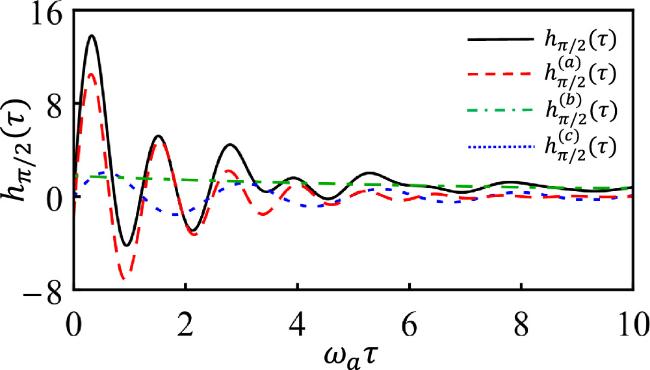
Similarly, we show the intensity-amplitude correlation for the level crossing case with g/ωq = 0.7 in figure 4. Comparing it with figure 3(a), one finds that the dominant oscillation still comes from ${h}_{\pi /2}^{(a)}(\tau )$ with the frequency of Ω, indicating that the small shift in frequency is due to the deviation in the coefficient ⟨$Psi$0∣(a + a†)∣$Psi$3⟩. The increase in amplitude is due to the decrease in the decay rate (2A + Γ30)/4 at g/ωq = 0.7. Furthermore, the increase of α13 highlights the oscillation from ${h}_{\pi /2}^{(c)}(\tau )$. Despite the relative amplitude ∣α13∣2 of ${h}_{\pi /2}^{(c)}(\tau )$ being less than ∣α03∣2 for ${h}_{\pi /2}^{(a)}(\tau )$, we can already identify a damped oscillation with frequency Ω/2 and decay rate (A + 2Γ10)/4 in the intensity-amplitude correlation.
Figure 4. The analytical results for the intensity-amplitude correlation function hπ/2(τ) and its decompositions. The parameters are the same as figure 2. |
4. Conclusion
In this paper, we have investigated the non-Gaussian features of a double qubit-cavity coupling system in the regime of ultrastrong coupling (USC). The ultrastrong coupling between the qubits and the cavity renders the rotating wave approximation inapplicable, necessitating the inclusion of counter-rotating wave terms to accurately describe the system's dynamics. Subsequently, we observed an anti-crossing splitting between levels three and four in the energy spectrum around g/ωq = 0.2, while the second and third levels exhibited level crossing at g/ωq = 0.7. Through aligning the frequency of the driving field to resonate with the transition from the ground state to the third energy level, we derived an equivalent four-level dressed state model. Modification of the dissipation term in the master equation with relaxation coefficients allowed us to obtain the steady state solution in analytic form. Furthermore, we discussed the non-Gaussian features of the output field based on the intensity-amplitude correlation function. While the output light does not exhibit squeezing, its intensity-amplitude correlation may violate the classical inequality, indicating non-Gaussian characteristics. We found that increasing the driving or coupling strength further enhances the non-Gaussian features of the system. To understand the physical origin of these findings, we provided the analytical result of the intensity-amplitude correlation function. The results of this study are instructive for the experimental preparation of non-Gaussian light.