


1. Introduction
Recently, a plethora of experimental and theoretical investigations have been conducted on magnetic composite nanostructures. These studies were motivated by the broad range of potential technological applications of these nanostructures. For instance, a combination of gold, polypyrene, and nickel has shown promise for magnetic alignment and wireless manipulation [1]. Similarly, composite systems, such as cobalt–copper and iron–cobalt–nickel–copper, have demonstrated their utility in magnetic field sensing and spintronic nanodevices [2–4]. Other applications include photochemical conversion and hydrogen generation using silver and zinc oxide [5], DNA molecule detection using cadmium telluride–gold–cadmium telluride [6], magnetic control of biomolecule desorption using iron–cobalt and copper [7], exchange coupled patterned media utilizing nickel and cobalt–platinum [8], nanosensors employing gold and cobalt [9], catalytic activities facilitated by platinum and nickel [10], and enhanced oxygen reduction reaction activity through the combination of cobalt and platinum [11]. Furthermore, these magnetic composite nanostructures have been found to exhibit a multitude of intriguing phenomena, adding to their scientific significance and potential for further exploration.
The magnetic properties of nanostructures are heavily influenced by their morphology and structural directions, specifically the radial direction for core–shell formation and the longitudinal direction for multisegmented structures. Consequently, nanostructures containing two or more magnetic and/or non-magnetic materials are distributed to achieve the desired radial or longitudinal orientation. Numerous studies have focused on investigating the thermal and magnetic behavior of these structures, particularly those involving core–shell and/or multisegmented configurations. Experimentally, the core/shell nanostructures, such as core/shell nanowires and core/shell nanotubes have been widely studied [12–19]. Furthermore, by using a variety of theoretical techniques, mainly effective-field theory (EFT) [20–28], Bethe Lattice [29–31], mean-field theory (MFT) [32–35], and Monte Carlo simulations (MCS) [36–43], and the magnetic properties of core/shell nanostructures have also been studied. Similarly, magnetically segmented nanostructures composed of alternating ferromagnetic or non-magnetic materials have been extensively explored [44–50]. Moreover, the segmented nanostructures with ferromagnetic–ferromagnetic and ferromagnetic–non-magnetic segments have been studied using EFT [51–53]. The EFT technique, first introduced by Honmura and Kaneyoshi [54], has been widely developed and applied to various magnetic systems, including thin films, nanostructures, and superlattices, and it is believed to give more exact results compared to the standard MFT.
On the other hand, extensive research has been conducted on diluted nanowires and nanotubes within the framework of the Ising model [27, 51, 55–60]. Theoretical techniques have been employed to investigate the phase diagrams and hysteresis behavior of these nanostructures when subjected to dilution. Furthermore, mixed-spin Ising systems, an extension of the standard spin-1/2 Ising model, have garnered significant attention from researchers because of their more complex critical behavior in comparison to single-spin systems. One of the earliest, simplest, and most extensively studied standard mixed-spin Ising systems is the mixed-spin (1/2-1) system. As a result, with the growth in the quantity of segments and interactions within the crystal lattice, the outcomes achieved become more diverse and captivating. Therefore, we studied the influence of segment dilution on the magnetic and hysteretic properties of ferrimagnetic (1/2-1) segmented Ising nanowire.
The layout of this work is organized as follows: the subsequent section provides an introduction to the model and presents the EFT. The dependence of magnetic properties on the dilution parameter is discussed in section 4 . The final section offers a comprehensive summary and conclusions of the findings.
2. Model and methods
Consider a multisegmented nanostructure with a non-magnetic/non-magnetic segment, as shown in figure 1, where the nanostructure consists of a surface shell and a core. Each site on the figure is occupied by an Ising spin, which is connected to the two nearest-neighbor spins in the above and below sections. These segments are referred to as a non-magnetic segment S1/2, a non-magnetic segment S1, and an inter segment. The system's Hamiltonian is provided by
$\begin{eqnarray}H={H}_{{\rm{I}}{\rm{N}}{\rm{T}}}+{H}_{1}+{H}_{1/2}.\end{eqnarray}$
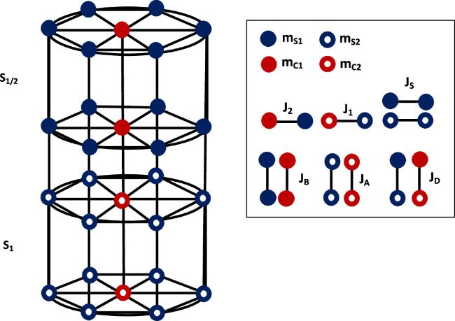
Figure 1. A schematic representation of segmented Ising nanowire. The S1/2 and S1 indicate non-magnetic segments for spin-1/2 and spin-1 segments, respectively. Moreover, the blue and red colors show the location of the shell and core non-magnetic atoms. |
In this equation, ${H}_{{\rm{I}}{\rm{N}}{\rm{T}}}$ encodes the interaction of the intra-segment spins of the system. It is given by:
$\begin{eqnarray}{{\rm{H}}}_{{\rm{INT}}}=-{J}_{D}\left(\displaystyle \sum _{\left\langle k{k}^{{\rm{{\prime} }}}\right\rangle }{S}_{k}{\sigma }_{{k}^{{\rm{{\prime} }}}}{\xi }_{k}{\xi }_{{k}^{{\rm{{\prime} }}}}+\displaystyle \sum _{\left\langle i{i}^{{\rm{{\prime} }}}\right\rangle }{S}_{i}{\sigma }_{{i}^{{\rm{{\prime} }}}}{\xi }_{i}{\xi }_{{i}^{{\rm{{\prime} }}}}\right).\end{eqnarray}$
The second term ${H}_{1}$ introduces the spin-1 segment interactions, and reads as $\begin{eqnarray}\begin{array}{c}{H}_{1}=-{J}_{S}\displaystyle \sum _{\left\langle {ij}\right\rangle }{{\rm{S}}}_{i}{{\rm{S}}}_{j}{\xi }_{i}{\xi }_{j}-{J}_{1}\displaystyle \sum _{\left\langle {ik}\right\rangle }{{\rm{S}}}_{i}{{\rm{S}}}_{k}{\xi }_{i}{\xi }_{k}\\ -\,{J}_{A}\left(\displaystyle \sum _{\left\langle k{k}^{{\rm{{\prime} }}{\rm{{\prime} }}}\right\rangle }{{\rm{S}}}_{k}{{\rm{S}}}_{{k}^{{{\rm{{\prime} }}{\rm{{\prime} }}}^{}}}{\xi }_{k}{\xi }_{{k}^{{{\rm{{\prime} }}{\rm{{\prime} }}}^{}}}+\displaystyle \sum _{\left\langle {{ii}}^{{\rm{{\prime} }}{\rm{{\prime} }}}\right\rangle }{{\rm{S}}}_{i}{{\rm{S}}}_{{i}^{{{\rm{{\prime} }}{\rm{{\prime} }}}^{}}}{\xi }_{i}{\xi }_{{i}^{{{\rm{{\prime} }}{\rm{{\prime} }}}^{}}}\right)\\ -\,{\rm{\Delta }}\left(\displaystyle \sum _{i}{{\rm{S}}}_{i}^{2}{\xi }_{i}+\displaystyle \sum _{k}{{\rm{S}}}_{k}^{2}{\xi }_{k}+\displaystyle \sum _{{i}^{{{\rm{{\prime} }}{\rm{{\prime} }}}^{}}}{{\rm{S}}}_{{i}^{{\rm{{\prime} }}{\rm{{\prime} }}}}^{2}{\xi }_{{i}^{{\rm{{\prime} }}{\rm{{\prime} }}}}+\displaystyle \sum _{{k}^{{\rm{{\prime} }}{\rm{{\prime} }}}}{{\rm{S}}}_{{k}^{{{\rm{{\prime} }}{\rm{{\prime} }}}^{}}}^{2}{\xi }_{{k}^{{{\rm{{\prime} }}{\rm{{\prime} }}}^{}}}\right)\\ -\,h\left(\displaystyle \sum _{i}{{\rm{S}}}_{i}{\xi }_{i}+\displaystyle \sum _{k}{{\rm{S}}}_{k}{\xi }_{k}+\displaystyle \sum _{{i}^{{\rm{{\prime} }}{\rm{{\prime} }}}}{{\rm{S}}}_{{i}^{{{\rm{{\prime} }}{\rm{{\prime} }}}^{}}}{\xi }_{{i}^{{{\rm{{\prime} }}{\rm{{\prime} }}}^{}}}+\displaystyle \sum _{{k}^{{{\rm{{\prime} }}{\rm{{\prime} }}}^{}}}{{\rm{S}}}_{{k}^{{{\rm{{\prime} }}{\rm{{\prime} }}}^{}}}{\xi }_{{k}^{{{\rm{{\prime} }}{\rm{{\prime} }}}^{}}}\right).\end{array}\end{eqnarray}$
The last term ${H}_{1/2}$ introduces the spin-1/2 segment interactions, and reads as $\begin{eqnarray}\begin{array}{c}{H}_{1/2}=-{J}_{S}\displaystyle \sum _{\left\langle {i}^{{\rm{{\prime} }}}{j}^{{\rm{{\prime} }}}\right\rangle }{\sigma }_{{i}^{{\rm{{\prime} }}}}{\sigma }_{{j}^{{\rm{{\prime} }}}}{\xi }_{{i}^{{\rm{{\prime} }}}}{\xi }_{{j}^{{\rm{{\prime} }}}}-{J}_{2}\displaystyle \sum _{\left\langle {i}^{{\rm{{\prime} }}}{k}^{{\rm{{\prime} }}}\right\rangle }{\sigma }_{{i}^{{\rm{{\prime} }}}}{\sigma }_{{k}^{{\rm{{\prime} }}}}{\xi }_{{i}^{{\rm{{\prime} }}}}{\xi }_{{k}^{{\rm{{\prime} }}}}\\ -{J}_{B}\left(\displaystyle \sum _{\left\langle {{k}^{{\rm{{\prime} }}}k}^{{{\rm{{\prime} }}{\rm{{\prime} }}}^{}}\right\rangle }{\sigma }_{{k}^{{\rm{{\prime} }}}}{\sigma }_{{k}^{{{\rm{{\prime} }}{\rm{{\prime} }}}^{}}}{\xi }_{{k}^{{\rm{{\prime} }}}}{\xi }_{{k}^{{{\rm{{\prime} }}{\rm{{\prime} }}}^{}}}+\displaystyle \sum _{\left\langle {i}^{{\rm{{\prime} }}}{i}^{{\rm{{\prime} }}{\rm{{\prime} }}}\right\rangle }{\sigma }_{{i}^{{\rm{{\prime} }}}}{\sigma }_{{i}^{{{\rm{{\prime} }}{\rm{{\prime} }}}^{}}}{\xi }_{{i}^{{\rm{{\prime} }}}}{\xi }_{{i}^{{{\rm{{\prime} }}{\rm{{\prime} }}}^{}}}\right)\\ -h\left(\displaystyle \sum _{{i}^{{\rm{{\prime} }}}}{\sigma }_{{i}^{{\rm{{\prime} }}}}{\xi }_{{i}^{{\rm{{\prime} }}}}+\displaystyle \sum _{{k}^{{\rm{{\prime} }}}}{\sigma }_{{k}^{{\rm{{\prime} }}}}{\xi }_{{k}^{{\rm{{\prime} }}}}+\displaystyle \sum _{{i}^{{{\rm{{\prime} }}{\rm{{\prime} }}}^{}}}{\sigma }_{{i}^{{{\rm{{\prime} }}{\rm{{\prime} }}}^{}}}{\xi }_{{i}^{{{\rm{{\prime} }}{\rm{{\prime} }}}^{}}}+\displaystyle \sum _{{k}^{{{\rm{{\prime} }}{\rm{{\prime} }}}^{}}}{\sigma }_{{k}^{{{\rm{{\prime} }}{\rm{{\prime} }}}^{}}}{\xi }_{{k}^{{{\rm{{\prime} }}{\rm{{\prime} }}}^{}}}\right).\end{array}\end{eqnarray}$
The summations over all pairs of neighboring spins on the segmented nanowire are denoted by ⟨…⟩. The external magnetic field is represented by h, while the exchange interaction between two nearest-neighbor atoms at the surface shell is denoted by JS. The S1/2 segment is connected to the next S1 segment through an exchange interaction JD. In both the S1/2 and S1 segments, the surface and core atoms are coupled with exchange interactions J1 and J2. Additionally, in the S12 segment, the surface atoms and core atoms are coupled with the exchange interaction JB, while in the S1 segment, the surface atoms and core atoms are coupled with the exchange interaction JA. The parameter ${\xi }_{\alpha }\left(\alpha ={i},{j},{k},{i}^{\prime} ,{j}^{\prime} ,{{k}^{\prime} ,{i}}^{^{\prime\prime} },{{k}}^{^{\prime\prime} }\right)$ is a site occupancy number that is 1 or zero, depending on whether the site is occupied or not. Since only the non-magnetic layer is diluted in the present system, ${\xi }_{\alpha }$ takes unity with a probability p when the site α is occupied by a magnetic atom and takes 0 with a probability (1−p) when the site α on the non-magnetic layer is occupied by a non-magnetic atom. The study examined the probability parameters pa and pb for segments S12 and S1, respectively. The exchange interaction values (JA, JB, J1, J2, JS, JD) were set at 1. Here, JD is selected to be the reduced unit. The investigation focused on how the segment dilution parameters pa and pb affected the nanowires' magnetic properties.
The starting point for the statistics of a multisegment system is the exact relation, as presented by Callen [61]. As discussed in [62, 63], for the evaluation of the mean values $\left\langle {\sigma }_{\alpha }\right\rangle $ and $\left\langle {{\rm{S}}}_{\alpha }\right\rangle ,$ we can use the exact Ising spin identities and the differential operator technique introduced by Honmura and Kaneyoshi [54, 64]. Hence, within the framework of the EFT, we can obtain the core and surface magnetizations. However, if we try to exactly treat all the spin–spin correlations for that set of equations, the problem quickly becomes untractable. A first obvious attempt to deal with this is to ignore correlations; the decoupling approximations. Based on the approximation, we obtained coupled equations for the longitudinal magnetizations mS1 and mC1 at the S1 segment and mC2 and mS2 at the S12 segment magnetizations:
$\begin{eqnarray}\begin{array}{l}{m}_{{\rm{S}}1}={\left[{p}_{b}\left\{1+{m}_{{\rm{S}}1}\,\sinh \left(A\right)+{q}_{{\rm{S}}1}\left(\cosh \left(A\right)-1\right)\right\}+1-{p}_{b}\right]}^{2}\\ \left[\times \,[{p}_{b}\left\{1+{m}_{{\rm{C}}1}\,\sinh \left(B\right)+{q}_{{\rm{C}}1}\left(\cosh \left(B\right)-1\right)\right\}+1-{p}_{b}\right]\\ \left[\times \,[{p}_{a}\left\{\cosh \left(C\right)+2{m}_{{\rm{S}}2}{\rm{s}}{\rm{i}}{\rm{n}}{\rm{h}}\left(C\right)\right\}+1-{p}_{a}\right]\\ \left[\times \,[{p}_{b}\left\{1+{m}_{{\rm{S}}1}\,\sinh \left(D\right)+{q}_{{\rm{S}}1}\left(\cosh \left(D\right)-1\right)\right\}+1-{p}_{b}\right]\\ \times \,{F}_{1}{\left.\left(x+h\right)\right|}_{x=0},\end{array}\end{eqnarray}$
$\begin{eqnarray}\begin{array}{l}{q}_{{\rm{S}}1}={\left[{p}_{b}\left\{1+{m}_{{\rm{S}}1}\,{\rm{s}}{\rm{i}}{\rm{n}}{\rm{h}}\left(A\right)+{q}_{{\rm{S}}1}\left(\cosh \left(A\right)-1\right)\right\}+1-{p}_{b}\right]}^{2}\\ \left[\times \,[{p}_{b}\left\{1+{m}_{{\rm{C}}1}\,{\rm{s}}{\rm{i}}{\rm{n}}{\rm{h}}\left(B\right)+{q}_{{\rm{C}}1}\left(\cosh \left(B\right)-1\right)\right\}+1-{p}_{b}\right]\\ \left[\times \,[{p}_{a}\left\{\cosh \left(C\right)+2{m}_{{\rm{S}}2}{\rm{s}}{\rm{i}}{\rm{n}}{\rm{h}}\left(C\right)\right\}+1-{p}_{a}\right]\\ \left[\times \,[{p}_{b}\left\{1+{m}_{{\rm{S}}1}\,{\rm{s}}{\rm{i}}{\rm{n}}{\rm{h}}\left(D\right)+{q}_{{\rm{S}}1}\left(\cosh \left(D\right)-1\right)\right\}+1-{p}_{b}\right]\\ \times \,{F}_{2}{\left.\left(x+h\right)\right|}_{x=0},\end{array}\end{eqnarray}$
$\begin{eqnarray}\begin{array}{l}{m}_{\mathrm{C1}}={\left[{p}_{b}\left\{1+{m}_{\mathrm{S1}}\,\sinh \left(B\right)+{q}_{\mathrm{S1}}\left(\cosh \left(B\right)-1\right)\right\}+1-{p}_{b}\right]}^{6}\\ \left[\times \,[{p}_{a}\left\{\cosh \left(C\right)+{{\rm{2}}m}_{\mathrm{C2}}\,\sinh \left(C\right)\right\}+1-{p}_{a}\right]\\ \left[\times \,[{p}_{b}\left\{1+{m}_{\mathrm{C1}}\,\sinh \left(D\right)+{q}_{{\rm{C}}1}\left(\cosh \left(D\right)-1\right)\right\}+1-{p}_{b}\right]\\ \times \,{F}_{1}{\left.\left(x+h\right)\right|}_{x=0},\end{array}\end{eqnarray}$
$\begin{eqnarray}\begin{array}{l}{q}_{C1}={\left[{p}_{b}\left\{1+{m}_{{\rm{S}}1}\,{\rm{s}}{\rm{i}}{\rm{n}}{\rm{h}}\left(B\right)+{q}_{{\rm{S}}1}\left(\cosh \left(B\right)-1\right)\right\}+1-{p}_{b}\right]}^{6}\\ \left[\times \,[{p}_{a}\left\{\cosh \left(C\right)+2{m}_{{\rm{C}}2}{\rm{s}}{\rm{i}}{\rm{n}}{\rm{h}}\left(C\right)\right\}+1-{p}_{a}\right]\\ \left[\times \,[{p}_{b}\left\{1+{m}_{{\rm{C}}1}\,{\rm{s}}{\rm{i}}{\rm{n}}{\rm{h}}\left(D\right)+{q}_{{\rm{C}}1}\left(\cosh \left(D\right)-1\right)\right\}+1-{p}_{b}\right]\\ \times \,{F}_{2}{\left.\left(x+h\right)\right|}_{x=0},\end{array}\end{eqnarray}$
$\begin{eqnarray}\begin{array}{l}{m}_{{\rm{S}}2}={\left[{p}_{a}\left\{\cosh \left(A\right)+2{m}_{{\rm{S}}2}{\rm{s}}{\rm{i}}{\rm{n}}{\rm{h}}\left(A\right)\right\}+1-{p}_{a}\right]}^{2}\\ \left[\times \,[{p}_{a}\left\{\cosh \left(E\right)+2{m}_{{\rm{C}}2}{\rm{s}}{\rm{i}}{\rm{n}}{\rm{h}}\left(E\right)\right\}+1-{p}_{a}\right]\\ \left[\times \,[{p}_{b}\left\{1+{m}_{{\rm{S}}1}\,\sinh \left(C\right)+{{\rm{q}}}_{{\rm{S}}1}\left(\cosh \left(C\right)-1\right)\right\}+1-{p}_{b}\right]\\ \left[\times \,[{p}_{a}\left\{\cosh \left(F\right)+2{m}_{{\rm{S}}2}{\rm{s}}{\rm{i}}{\rm{n}}{\rm{h}}\left(F\right)\right\}+1-{p}_{a}\right]G{\left.\left(x+h\right)\right|}_{x=0},\end{array}\end{eqnarray}$
$\begin{eqnarray}\begin{array}{l}{m}_{C2}={\left[{p}_{a}\left\{\cosh \left(B\right)+2{m}_{{\rm{S}}2}{\rm{s}}{\rm{i}}{\rm{n}}{\rm{h}}\left(B\right)\right\}+1-{p}_{a}\right]}^{6}\\ \left[\times \,[{p}_{b}\left\{1+{m}_{{\rm{C}}1}\,\sinh \left(C\right)+{{\rm{q}}}_{{\rm{C}}1}\left(\cosh \left(C\right)-1\right)\right\}+1-{p}_{b}\right]\\ \left[\times \,[{p}_{a}\left\{\cosh \left(D\right)+2{m}_{{\rm{C}}2}{\rm{s}}{\rm{i}}{\rm{n}}{\rm{h}}\left(D\right)\right\}+1-{p}_{a}\right]\\ \times \,G{\left.\left(x+h\right)\right|}_{x=0}.\end{array}\end{eqnarray}$
Here, the coefficients A, B, C, D, E, and F are ${{J}}_{{S}}{\rm{\nabla }},$ ${{J}}_{1}{\rm{\nabla }},$ ${{J}}_{{D}}{\rm{\nabla }},$ ${{J}}_{{A}}{\rm{\nabla }},$ ${{J}}_{2}{\rm{\nabla }}$, and ${{J}}_{{B}}{\rm{\nabla }},$ respectively. Moreover, ${\rm{\nabla }}=\partial /\partial x$ is the differential operator. The functions ${{F}}_{1}\left({x}\right),$ ${{F}}_{2}\left({x}\right)$, and ${G}\left({x}\right)$ are defined as
$\begin{eqnarray}{F}_{1}\left(x\right)=\displaystyle \frac{2\,\sinh \left[\beta \left(x+h\right)\right]}{\exp \left(-\beta {\rm{\Delta }}\right)+2\,\cosh \left[\beta \left(x+h\right)\right]},\end{eqnarray}$
$\begin{eqnarray}{F}_{2}\left(x\right)=\displaystyle \frac{2\,\cosh \left[\beta \left(x+h\right)\right]}{\exp \left(-\beta {\rm{\Delta }}\right)+2\,\cosh \left[\beta \left(x+h\right)\right]},\end{eqnarray}$
$\begin{eqnarray}G\left(x\right)=\displaystyle \frac{1}{2}\,\tan \,h\left[\displaystyle \frac{1}{2}\beta \left(x+h\right)\right].\end{eqnarray}$
Here, $\beta =1/{k}_{{\rm{B}}}T,$ where T is the absolute temperature, and kB is the Boltzmann constant.
By using the definitions of the order parameters in equations (2a ), the segment and total magnetizations per site can be defined as
$\begin{eqnarray}{M}_{1/2}=\frac{{p}_{a}{m}_{C2}+6{p}_{a}{m}_{S2}}{7{p}_{a}},\end{eqnarray}$
$\begin{eqnarray}{M}_{1}=\frac{{p}_{b}{m}_{C1}+6{p}_{b}{m}_{S1}}{7{p}_{b}},\end{eqnarray}$
$\begin{eqnarray}{{M}}_{{\rm{T}}}=\displaystyle \frac{\left({{p}}_{{b}}\,{{m}}_{{\rm{C}}1}+{{p}}_{{a}}{{m}}_{{\rm{C}}2}+\left(6\,{{p}}_{{b}}\,{{m}}_{{\rm{S1}}}+6\,{{p}}_{{a}}{{m}}_{{\rm{S}}2}\right)\right)}{7\,{{p}}_{{a}}+7{{p}}_{{b}}}.\end{eqnarray}$
By solving these equations, we can get the phase diagrams and hysteresis behavior of the system. We will perform the calculations in the next section.
3. Numerical results and discussion
In this section, we examine the magnetic properties and hysteresis characteristics, namely the hysteresis loop area (HLA), coercivity field (HC) and remanent magnetization (Mr). This system is affected by the temperature (T), segment dilutions (pa and pb), and crystal field (Δ) parameters. The phase diagrams are examined on the planes of (T, pa), (T, pb), (Δ, T), and (pb, pa). To examine the impact of segment dilution on the system, the article maintains a consistent set of interaction parameters, namely JA, JB, J1, J2, JD, and JS. This approach allows a focused analysis of the effect of segment dilution without the confounding influence of varying interaction parameters.
3.1. Magnetization curves
The investigation of the temperature dependence of both the segment magnetizations and the total magnetization allows the determination of the phase transition points. This research provides valuable insights into the nature of these transitions, whether they are continuous or discontinuous. To illustrate the interaction, figures 2(a)–(d) present the behavior of the segment magnetizations and the total magnetization (MT) as a function of temperature for different values of the interaction parameters. Within these figures, TC and Tt represent the second- and first- order phase transition temperatures, respectively. Figure 2(a) specifically depicts the behavior of the non-magnetic (nm) phase. At zero temperature, the values of M12 and M1 are 0.5 and 0.0, respectively. As the temperature increases, these values continuously decrease until reaching zero at TC. Consequently, a second-order phase transition occurs at TC = 0.96, leading to a transition from the nm phase to the p phase. Figure 2(b) focuses on the behavior of phase i. At zero temperature, the values of M12 and M1 are 0.5 and 1.0, respectively. Similar to the previous case, as the temperature increases, these values continuously decrease until reaching zero at TC. Thus, a second-order phase transition occurs at TC = 2.1, resulting in a phase transition from phase i to phase p. In figure 2(c), the behavior of the first-order phase transition is depicted. The values of M12 and M1 are 0.5 and 1.0, respectively, at zero temperature. As the temperature rises, M1 gradually decreases until it reaches Tt, where it experiences a sudden drop. This abrupt decrease signifies the occurrence of a first-order phase transition at Tt = 0.6. The transition observed in this case is from phase i to phase p. On the other hand, figure 2(d) illustrates the presence of both first- and second-order phase transition behavior. At zero temperature, M12 is 0.5 and M1 is 1.0. As the temperature increases, M1 undergoes a sudden decrease to zero at Tt = 0.38, while M12 remains at 0.5, indicating a transition to the nm phase. Subsequently, with further temperature increase, M12 gradually diminishes to zero until TC, leading to a transition to the p phase. In this scenario, the phase transition occurs from the nm phase to the p phase at TC = 1.0.
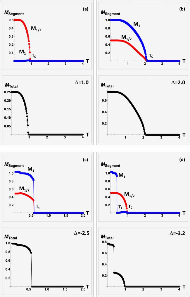
Figure 2. The thermal variation of the total and partial magnetizations for fixed values of J1 = J2 = JA = JB = JD = JS = 1 and pa = pb = 1. (a) Exhibiting a second-order phase transition from the nm phase to the p phase for Δ = 1.0. (b) Exhibiting a second-order phase transition from the i phase to the p phase for Δ = 2.0. (c) Exhibiting a first-order phase transition from the nm phase to the p phase for Δ = −2.5. (d) Exhibiting first-order phase transitions from the i phase to the nm phase and then second-order phase transitions from the nm phase to the p phase for Δ = −3.2. |
3.2. Influence of dilution parameters on the phase diagrams
The phase diagrams in the (T, pa) and (T, pb) planes for various values of pa and pb are plotted in figure 3. The results indicate that all phase transitions are second-order transitions from the ferrimagnetic (i) phase to the paramagnetic (p) phase. The critical temperature is slightly affected by changes in pa, as observed in figures 3(a) and (b). In figure 3(c), the p phase is the only phase present at low values of pa, and as pa increases, the critical temperature increases linearly with a larger slope. Similarly, in figures 3(d)–(f), the critical temperature increases linearly with the increase in pb for all values of pa. However, in figure 3(f), there is no i phase at low pb values, similar to figure 3(c). To investigate the impact of the concentration of magnetic atoms at the S12 and S1 segments, specifically pa and pb, on the behavior of the system, an analysis was conducted.
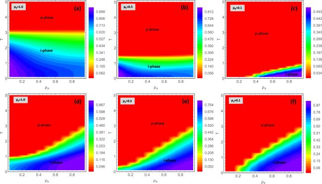
Figure 3. The phase diagrams are depicted on the (T, pa) and (T, pb) for J1 = J2 = JA = JB = JD = JS = 1, Δ = 0.0, and encompass a range of dilution values. The dilution values examined are: (a) pb = 1.0, (b) pb = 0.5, (c) pb = 0.1, (d) pa = 1.0, (e) pa = 0.5, and (f) pa = 0.1. |
The phase diagrams in the (T, Δ) plane were presented for different values of pa and pb, namely pa = pb = 1, pa = 1, pb = 0.1, and pa = 0.1, pb = 1.0, while varying the parameter Δ (figure 4). It is evident from the diagrams that the nature of the phase transition is influenced by the changes in the dilution parameters. Notably, the system exhibits a first-order phase transition in the cases of pa = pb =1 and pa = 1, pb = 0.1. In figure 4(a), the transition occurs between the nm phase and the i phase at high negative values of the crystal field. In the nm phase, the system demonstrates both paramagnetic and ferromagnetic behavior; hence, the nm phase exists in figure 4(a). In this behavior, the S1 segment magnetizations mC1 and mS1 have zero values, while the S1/2 segment magnetizations mC2 and mS2 show non-zero values. On the other hand, the first-order phase transition in figure 4(b) takes place between the i phase and the p phase. In the case of pa = 0.1, pb = 1.0, a second-order phase transition is observed, and it occurs at approximately the same critical temperature for all crystal field values.
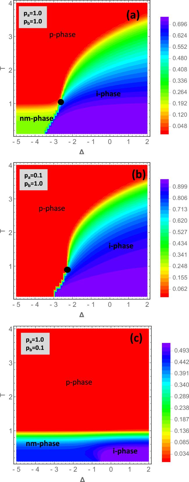
Figure 4. The phase diagrams are depicted on the (Δ, T) for J1 = J2 = JA = JB = JD = JS = 1, and encompass a range of dilution values. The tricritical point is marked with filled circles. The dilution values examined are: (a) pa = 1.0 and pb = 1.0, (b) pa = 0.1 and pb = 1.0, (c) pa = 1.0, and pb = 0.1. |
Finally, in figure 5, we have presented the variation of the S12 segment dilution pa versus the S1 segment dilution pb, and for different crystal field values, namely Δ = 2⊡0, Δ = 0⊡0, Δ = 2⊡0, and Δ = 4⊡0. Upon examination of figures 5(a) and (b), it becomes evident that the p phase is present at low values of pa and pb, while the i phase is detected at all other values. In the phase diagram obtained for the case where the crystal field is at Δ = 2⊡0 and presented in figure 5(c), it is observed that there are three phases in the system: p phase, i phase, and nm phase. The p phase was found at low values of pa, while the nm phase was observed at high values of pa. The i phase was obtained at high values of pb. In the phase diagram obtained for Δ = 4⊡0 in figure 5(d), it was determined that there was no i phase and only the p and nm phases were present.
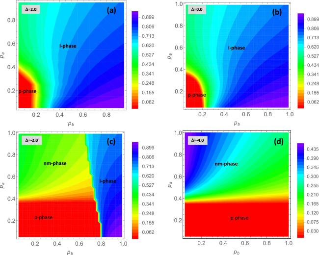
Figure 5. The phase diagrams are depicted on the (pb, pa) for J1 = J2 = JA = JB = JD = JS = 1 and T = 0.1, and encompass a range of crystal field values. The crystal field values examined are: (a) Δ = 2.0, (b) Δ = 0.0, (c) Δ = −2.0, and (d) Δ = −4.0. |
3.3. Hysteresis characteristics: effects of temperature, segment dilutions, and crystal field
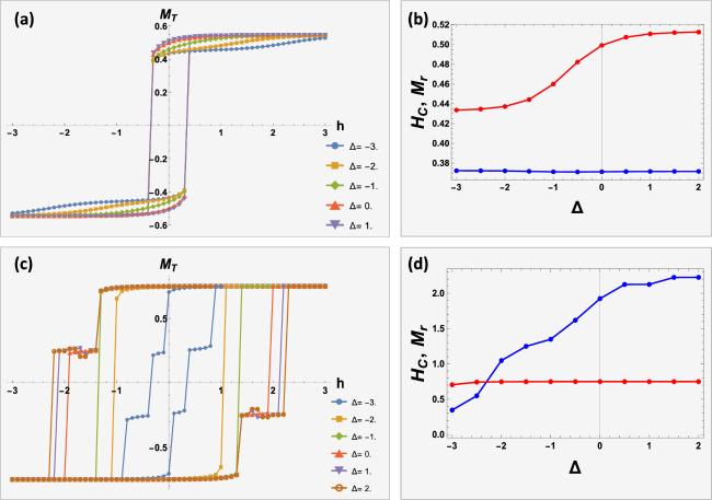
In this subsection, the hysteresis characteristics of the system are examined with regard to their dependence on temperature, segment dilutions, and crystal field and are presented in figures 6–8. The investigation of hysteresis loops in low-dimensional nanostructures has been conducted through the utilization of MCS [43, 65–69]. Kantar [70] examined the thermal and magnetic properties of a hexagonal Ising nanowire and various other systems [25, 71] using EFT. When analyzing the hysteresis behavior in the figures, two different states of pb were taken into account, such as pb = 0.1 and pb = 1.0. Initially, the effect of increasing pa was examined for the pb = 0.1 case, which revealed a decrease in HLA as pa increased, as seen in figure 6(a). Upon analyzing the HC and Mr values corresponding to these pa values, it was found that the system was paramagnetic up to a certain value of pa, beyond which the values of these two parameters began to increase, as seen in figure 6(b). In contrast, the hysteresis behavior observed for the second case, where pb = 1.0, displayed distinct behavior. As the value of pa increases, the HLA becomes narrower and the HC and Mr tend to decrease, as seen in figures 6(c) and (d). The reason for this difference is that at small values of pb and pa, the system is in the paramagnetic region, and then at increasing values of pa, the system reaches the ferrimagnetic region. In this case, the dominant segment on the magnetic character of the system is the spin-1/2 segment. Figure 7 presents the variation of hysteresis characteristics with temperature for both pb = 0.1 and pb = 1.0. It is evident that as the temperature rises, the area enclosed by the hysteresis loop narrows, and the HC and Mr decrease until the hysteresis disappears below the critical temperature, indicating the loss of ferromagnetic properties at lower temperatures. At colder temperatures, a single hysteresis loop with a rectangular shape is observed, as the magnetization quickly reaches saturation. This results in the system displaying hard magnetic characteristics with a broad hysteresis loop. As the temperature increases, the loops begin to round due to fluctuations. The magnetizations no longer saturate after completing a cycle, and the slope of the increase decreases with rising temperature. At higher temperatures, the system exhibits soft magnetic characteristics with a smaller hysteresis loop, where all moments fluctuate with a relaxation time that is shorter than the measuring time. Consequently, the magnetization decreases to a point where less magnetic field is required to reverse the magnetic moments. Similar hysteresis loop behavior has been noted in nanostructure systems within both theoretical and experimental frameworks. In figure 8, the influence of the crystal area parameter on the hysteresis characteristics is examined. For pb = 0.1, the increase in crystal field did not alter the HLA, but the Mr increased within a specific crystal field range. Conversely, for pb = 1, the HC increased as the HLA increased.
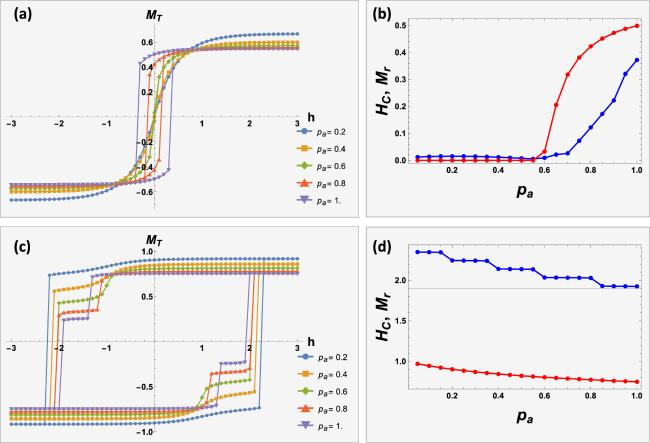
Figure 6. The dilution dependence of the hysteresis behavior for fixed values of J1 = J2 = JA = JB = JD = JS = 1, Δ = 0.0, and T = 0.5. (a) Magnetic hysteresis loops of nanowire for pa values ranging from 0 to 1 with a pb = 0.1. (b) For pb = 0.1, the dilution dependence of the coercive field and remanent magnetization. (c) Magnetic hysteresis loops of nanowire for pa values ranging from 0 to 1 with a pb = 1.0. (d) For pb = 1.0, the dilution dependence of the coercive field and remanent magnetization. |
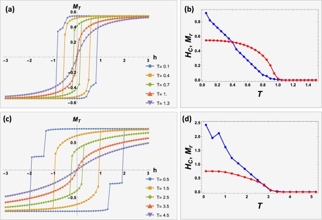
Figure 7. The temperature dependence of the hysteresis behavior for fixed values of J1 = J2 = JA = JB = JD = JS = 1, Δ = 0.0, and pa = 1.0. (a) Magnetic hysteresis loops of nanowire for T values ranging from 0 to 1.5 with a pb = 0.1. (b) For pb = 0.1, the temperature dependence of the coercive field and remanent magnetization. (c) Magnetic hysteresis loops of nanowire for T values ranging from 0 to 1.5 with a pb = 1.0. (d) For pb = 1.0, the temperature dependence of the coercive field and remanent magnetization. |
Figure 8. The crystal field dependence of the hysteresis behavior for fixed values of J1 = J2 = JA = JB = JD = JS = 1, T = 0.5, and pa = 1.0. (a) Magnetic hysteresis loops of nanowire for Δ values ranging from −3 to 2 with a pb = 0.1. (b) For pb = 0.1, the crystal field dependence of the coercive field and remanent magnetization. (c) Magnetic hysteresis loops of nanowire for Δ values ranging from −3 to 2 with a pb = 1.0. (d) For pb = 1.0, the crystal field dependence of the coercive field and remanent magnetization. |
4. Summary and conclusion
This paper discusses the magnetization curves, phase diagrams, and hysteresis characteristics of a system under different conditions using the EFT. Various phase transitions are observed, including second-order transitions from the nm phase to the p phase and first-order transitions from phase i to phase p. First-order phase transitions occur between the nm phase and the i phase, as well as between the i phase and the p phase in some phase diagrams. The variation of segment dilution parameters and crystal field also leads to the presence of different phases in the system. The hysteresis characteristics of the system are also analyzed, showing the effects of temperature, segment dilutions, and crystal field. The HLA, HC, and Mr are found to be influenced by these factors. As the temperature and segment dilutions increase, the HLA becomes narrower, and the HC and Mr decrease. The crystal field parameter also affects the hysteresis characteristics, with different behavior observed for different values of segment dilutions.