


1. Introduction
Fractional calculus (FC) and fractional order mathematical models have gained substantial popularity in numerous studies for modeling diverse applications in fluid mechanics, physics of plasmas, engineering, and applied sciences. This is primarily attributed to their capacity to effectively and comprehensively represent various issues and applications. The available literature encompasses a wide range of studies, including those focused on modeling biological phenomena and diseases [1, 2], modeling diffusive type circuits [3, 4], conducting an extensive survey on the applications of FC and fractional order derivative-based techniques in computer vision [5], and investigating sensors, analog, and digital filters [6]. The fundamental framework for FC that several pioneers recommended, as well as their perspectives on generalized calculus. FC has been used in various fields where the fascinating and simulating implications linked with temporal and hereditary features may be found [7–12]. The solution of fractional differential equations that represent complex issues in everyday life is crucial for uncovering their physical core.
Fractional partial differential equations (PDEs) can address intricate engineering and physical issues more effectively than typical integer-order PDEs, showcasing the superior capabilities of fractional PDEs (FPDEs) as demonstrated in references [13–16]. As well as their ability in modeling the complex systems related to the genetic or memory properties [17–20]. Also, an essential advantage over traditional differential equations is their handling of non-local interactions and long-term time dependence.
One of the PDEs that describes a broad spectrum of physical nonlinear phenomena as well as engineering materials is the well-known Korteweg–de Vries (KdV) equation [21–26]. This equation and its family, whether it contains third-order dispersion [27–29] or fifth-order dispersion [30–32] or other physical effects such as collision and viscosity forces, have effectively elucidated numerous nonlinear structures that emerge and propagate in diverse physical and engineering systems, including fluid physics and plasma physics. It has been widely used, especially in interpreting soliton and cnoidal waves propagating in various plasma systems [33–36]. Furthermore, it succeeded in explaining some ambiguity that may appear in the properties of soliton and shock waves that propagate in numerous plasma models. Many researchers have demonstrated that this ambiguity may be attributed to the fact that these models may encompass various physical effects that influence the dynamics of these waves, including the collisions between plasma charges particles and/or neutral atoms as well as the viscosity of some charged plasma particles, and many other physical effects [37–44].
The forced KdV (FKdV) equation was utilized to examine the influence of bottom configurations on free-surface waves in a two-dimensional channel flow. Studying shallow-water waves highlights the significance of bottom topography in determining wave motion characteristics [45, 46]. Waves with a wavelength in water less than one-quarter of their actual wavelength are categorized as shallow or long waves. As the bottom topography becomes more intricate, the interaction between it and solitary waves (SWs) unveils a rich tapestry of dynamic characteristics within the free surface waves. The free surface waves of a two-dimensional channel flow have been studied in cases where the stiff channel bottom has certain obstructions and for an incompressible and inviscid fluid [47, 48]. When fluid flows over an obstruction, the KdV equation's estimated forcing can be used to show how the free surface develops. When discussing the nonlinear Schrödinger equation and the nature of the sine Gordon equation, the FKdV equation is essential. The model above exhibits numerous applications in tightly interconnected domains of mathematics and physics. This equation is regarded as a vital tool for research into atmosphere dynamics, geostrophic turbulence, and magnetohydrodynamic waves, to name a few [49, 50]. The study yields promising findings about several physical phenomena, such as the propagation of shallow-water waves over rocks, the occurrence of tsunami waves over obstacles, the interaction between oceanic stratified flows and topographic impediments, and the study of acoustic waves on a crystal lattice.
This article incorporates the FKdV equation, which was first proposed and refined by Wu in 1987 [51], along with the free water surface elevation Φ ≡ Φ(X, T) observed during critical flow over a hole from the undisturbed water level1 ), the Froude number $({{ \mathcal F }}_{r})$ is significant hence its value reveals the type of critical flows over the localized restriction. Generally, the flow is classified as subcritical, supercritical, and transcritical for values less than, greater than, and equal to 1, respectively. Two different types of holes, namely those for n = 2 and n = 8, were explored in the stiff bottom topography b(X). In each of these situations, the hole is predicted to be broader and more flattened at the bottom than bell-shaped. In [52], the authors removed the surface air pressure from equation (1 ), and considered the following simplified form to FKdV equation3 ). The proposed methods involve the combination of the Yang transform (YT) with the homotopy perturbation technique (HPM) to produce the (YTHPM), as well as the combination of the adomian decomposition method (ADM) with YT to generate the (YTADM). These methods are used to obtain analytical approximations for non-integer evolution equations. It is known that the HPM was introduced for the first time by He [54, 55] in 1998, which in this technique, the solution is postulated to be the aggregate of an endless series that exhibits quick convergence toward exact outcomes. The mentioned technique has demonstrated efficacy in resolving and examining linear and nonlinear equations. Moreover, to create YTDM, the ADM and the Yang transform are merged. By eliminating the requirement to calculate the fractional integrals or fractional derivative in the recursive mechanism, the suggested method enables estimating the series terms easier than the conventional Adomian method [56].
$\begin{eqnarray}\displaystyle \frac{1}{c}{\partial }_{T}{\rm{\Phi }}+\left[({{ \mathcal F }}_{r}-1)-\displaystyle \frac{3}{2}\displaystyle \frac{{\rm{\Phi }}}{h}\right]{\partial }_{X}{\rm{\Phi }}-\displaystyle \frac{1}{6}{h}^{2}{\partial }_{X}^{3}{\rm{\Phi }}=\displaystyle \frac{1}{2}{\partial }_{X}f(X),\end{eqnarray}$
with $\begin{eqnarray*}f(X)=\displaystyle \frac{{\rho }_{a}(X)}{\rho g}+b(X),\end{eqnarray*}$
where f(X) represents the externally forcing term, “h” indicates the sea water depth, and ${{ \mathcal F }}_{r}$ represents the Froude number, which is also known as the critical parameter. Here, the surface air pressure is denoted by $\tfrac{{\rho }_{a}(X)}{\rho g}$, and stiff bottom topography is specified by $b(X)=\left(-0.1{{\rm{e}}}^{-\tfrac{{X}^{n}}{4}}-1\right)$. In equation ( $\begin{eqnarray}\begin{array}{l}\displaystyle \frac{1}{c}{\partial }_{T}{\rm{\Phi }}+\left[({{ \mathcal F }}_{r}-1)-\displaystyle \frac{3}{2}\displaystyle \frac{{\rm{\Phi }}}{h}\right]{\partial }_{X}{\rm{\Phi }}\\ \quad -\displaystyle \frac{1}{6}{h}^{2}{\partial }_{X}^{3}{\rm{\Phi }}-\displaystyle \frac{1}{2}{\partial }_{X}b(X)=0.\end{array}\end{eqnarray}$
By substituting an arbitrary order derivative for the time derivative in the current study, we get the following fractional-order forced KdV (FF-KdV) equation [53]: $\begin{eqnarray}\begin{array}{l}{D}_{T}^{\gamma }{\rm{\Phi }}+c\left[\left(({{ \mathcal F }}_{r}-1)-\displaystyle \frac{3}{2}\displaystyle \frac{{\rm{\Phi }}}{h}\right){\partial }_{X}{\rm{\Phi }}\right.\\ \quad \left.-\displaystyle \frac{1}{6}{h}^{2}{\partial }_{X}^{3}{\rm{\Phi }}-\displaystyle \frac{1}{2}{\partial }_{X}b(X)\right]=0,\end{array}\end{eqnarray}$
where 0 < γ ≤ 1 and the operator ${D}_{T}^{\gamma }\equiv \tfrac{{\partial }^{\gamma }}{\partial {T}^{\gamma }}$ indicates the Caputo fractional derivative having order γ. In this study, both Yang transform decomposition method (YTDM) and Yang homotopy perturbation method (YHPM) are introduced for analyzing the FF-KdV (The forthcoming parts of the manuscript are organized in the following manner: section 2 comprises a declarative declaration and several fundamental concepts. Sections 3 and 4 delineate the recommended procedures for the proposed techniques. Section 5 contains the application and illustrations for the suggested approach. Section 6 outlines the investigation's conclusion.
2. Preliminaries
Below are the definitions of Caputo's fractional derivative and various features of YT:
2.1. Definition
In the context of the Caputo sense, the fractional-order derivative is defined as follows
$\begin{eqnarray*}{D}_{T}^{\gamma }{\rm{\Phi }}=\displaystyle \frac{1}{{\rm{\Gamma }}(k-\gamma )}{\int }_{0}^{T}{\left(T-\vartheta \right)}^{k-\gamma -1}{{\rm{\Phi }}}^{(k)}{\rm{d}}\vartheta ,\end{eqnarray*}$
where k − 1 < γ ≤ k, k ∈ N, and Φ ≡ Φ(X, T).2.2. Definition
The YT of a function Φ(T) is defined as
$\begin{eqnarray}\begin{array}{c}{\bf{Y}}\{{\rm{\Phi }}(T)\}=M(u)={\int }_{0}^{\infty }{{\rm{e}}}^{\tfrac{-T}{u}}{\rm{\Phi }}(T){\rm{d}}T,\ T\gt 0,\\ u\in (-{T}_{1},{T}_{2}),\end{array}\end{eqnarray}$
with the inverse YT $\begin{eqnarray}{{\bf{Y}}}^{-1}\{M(u)\}={\rm{\Phi }}(T).\end{eqnarray}$
2.3. Definition
The YT of the function Φn(T) with nth derivative reads
$\begin{eqnarray}{\bf{Y}}\{{{\rm{\Phi }}}^{n}(T)\}=\displaystyle \frac{M(u)}{{u}^{n}}-\displaystyle \sum _{k=0}^{n-1}\displaystyle \frac{{{\rm{\Phi }}}^{k}(0)}{{u}^{n-k-1}},\ \forall \ n=1,2,3,\,\cdots \,.\end{eqnarray}$
2.4. Definition
The YT of the fractional-order derivative function Φγ(T) is given by
$\begin{eqnarray}{\bf{Y}}\{{{\rm{\Phi }}}^{\gamma }(T)\}=\displaystyle \frac{M(u)}{{u}^{\gamma }}-\displaystyle \sum _{k=0}^{n-1}\displaystyle \frac{{{\rm{\Phi }}}^{k}(0)}{{u}^{\gamma -(k+1)}},\ 0\lt \gamma \leqslant n.\end{eqnarray}$
3. Analysis of HPTM
We can provide the fundamental aspects of HPTM in the following points to comprehend the process of its application to the problem under study. To start, let us introduce the following problem
$\begin{eqnarray}\left\{\begin{array}{l}{D}_{T}^{\gamma }{\rm{\Phi }}={{ \mathcal P }}_{1}[X]{\rm{\Phi }}+{{ \mathcal Q }}_{1}[X]{\rm{\Phi }},\ \\ {\rm{\Phi }}(X,0)=\xi (X),\end{array}\right.\end{eqnarray}$
where 0 < γ ≤ 1, Φ ≡ Φ(X, T), ${D}_{T}^{\gamma }=\tfrac{{\partial }^{\gamma }}{\partial {T}^{\gamma }}$ indicates the Caputo fractional derivative, ${{ \mathcal P }}_{1}[X]$ and ${{ \mathcal Q }}_{1}[X],$ respectively, are the linear and nonlinear operators. On taking YT of either sides $\begin{eqnarray}{\bf{Y}}[{D}_{T}^{\gamma }{\rm{\Phi }}]={\bf{Y}}[{{ \mathcal P }}_{1}[X]{\rm{\Phi }}+{{ \mathcal Q }}_{1}[X]{\rm{\Phi }}],\end{eqnarray}$
$\begin{eqnarray}\displaystyle \frac{1}{{u}^{\gamma }}\{M(u)-u{\rm{\Phi }}(0)\}={\bf{Y}}[{{ \mathcal P }}_{1}[X]{\rm{\Phi }}+{{ \mathcal Q }}_{1}[X]{\rm{\Phi }}],\end{eqnarray}$
which leads to $\begin{eqnarray}M(u)=u{\rm{\Phi }}(0)+{u}^{\gamma }{\bf{Y}}[{{ \mathcal P }}_{1}[X]{\rm{\Phi }}+{{ \mathcal Q }}_{1}[X]{\rm{\Phi }}].\end{eqnarray}$
Implementing the inverse YT on either sides $\begin{eqnarray}{\rm{\Phi }}={\rm{\Phi }}(0)+{{\bf{Y}}}^{-1}[{u}^{\gamma }{\bf{Y}}[{{ \mathcal P }}_{1}[X]{\rm{\Phi }}+{{ \mathcal Q }}_{1}[X]{\rm{\Phi }}]].\end{eqnarray}$
Now, we proceed to apply the perturbation technique $\begin{eqnarray}\ {\rm{\Phi }}=\displaystyle \sum _{k=0}^{\infty }{\epsilon }^{k}{{\rm{\Phi }}}_{k},\end{eqnarray}$
with parameter ε ∈ [0, 1] and Φk ≡ Φk(X, T).The breakdown of nonlinear term is given by11 ) and (12 ) in equation (10 ), we have
$\begin{eqnarray}\ {{ \mathcal Q }}_{1}[X]{\rm{\Phi }}=\displaystyle \sum _{k=0}^{\infty }{\epsilon }^{k}{H}_{n}({\rm{\Phi }}),\end{eqnarray}$
with Hk(Φ) illustrating He's polynomials and given by $\begin{eqnarray}\ {H}_{n}({{\rm{\Phi }}}_{0},{{\rm{\Phi }}}_{1},\,\ldots ,\,{{\rm{\Phi }}}_{n})=\displaystyle \frac{1}{{\rm{\Gamma }}(n+1)}{D}_{\epsilon }^{k}{\left[{{ \mathcal Q }}_{1}\left(\displaystyle \sum _{k=0}^{\infty }{\epsilon }^{i}{{\rm{\Phi }}}_{i}\right)\right]}_{\epsilon =0},\end{eqnarray}$
where ${D}_{\epsilon }^{k}=\tfrac{{\partial }^{k}}{\partial {\epsilon }^{k}}.$ Using equations ( $\begin{eqnarray}\begin{array}{l}\ \displaystyle \sum _{k=0}^{\infty }{\epsilon }^{k}{{\rm{\Phi }}}_{k}(X,T)={\rm{\Phi }}(0)+\epsilon \left({{\bf{Y}}}^{-1}\left[{u}^{\gamma }{\bf{Y}}\{{{ \mathcal P }}_{1}\displaystyle \sum _{k=0}^{\infty }{\epsilon }^{k}{{\rm{\Phi }}}_{k}(X,T)\right.\right.\\ \quad \left.\left.+\,\displaystyle \sum _{k=0}^{\infty }{\epsilon }^{k}{H}_{k}({\rm{\Phi }})\}\right]\right).\end{array}\end{eqnarray}$
By matching either sides of the above equation in terms of power of ε, we get $\begin{eqnarray}\begin{array}{l}{\epsilon }^{0}:{{\rm{\Phi }}}_{0}(X,T)={\rm{\Phi }}(0),\\ {\epsilon }^{1}:{{\rm{\Phi }}}_{1}(X,T)={{\bf{Y}}}^{-1}\left[{u}^{\gamma }{\bf{Y}}({{ \mathcal P }}_{1}[X]{{\rm{\Phi }}}_{0}(X,T)+{H}_{0}({\rm{\Phi }}))\right],\\ {\epsilon }^{2}:{{\rm{\Phi }}}_{2}(X,T)={{\bf{Y}}}^{-1}\left[{u}^{\gamma }{\bf{Y}}({{ \mathcal P }}_{1}[X]{{\rm{\Phi }}}_{1}(X,T)+{H}_{1}({\rm{\Phi }}))\right],\\ \vdots \\ {\epsilon }^{k}:{{\rm{\Phi }}}_{k}(X,T)={Y}^{-1}\left[{u}^{\gamma }Y({{ \mathcal P }}_{1}[X]{{\rm{\Phi }}}_{k-1}(X,T)+{H}_{k-1}({\rm{\Phi }}))\right],\end{array}\end{eqnarray}$
where k > 0 and k ∈ N.Lastly, the approximate solution Φk(X, T) reads
$\begin{eqnarray}{\rm{\Phi }}(X,T)=\mathop{\mathrm{lim}}\limits_{M\to \infty }\displaystyle \sum _{k=1}^{M}{{\rm{\Phi }}}_{k}(X,T).\end{eqnarray}$
4. Analysis of YTDM
The following problem is considered to demonstrate the core theory and solution process of YTDM23 ) and (25 ) into (22 ), we get
$\begin{eqnarray}\left\{\begin{array}{l}{D}_{T}^{\gamma }{\rm{\Phi }}={{ \mathcal P }}_{1}+{{ \mathcal Q }}_{1},\\ {\rm{\Phi }}(X,0)={\rm{\Phi }}(X),\end{array}\right.\end{eqnarray}$
where 0 < γ ≤ 1 and ${D}_{T}^{\gamma }=\tfrac{{\partial }^{\gamma }}{\partial {T}^{\gamma }}$ signifies the Caputo fractional derivative, ${{ \mathcal P }}_{1}\equiv {{ \mathcal P }}_{1}(X,T)$ and ${{ \mathcal Q }}_{1}\equiv {{ \mathcal Q }}_{1}(X,T)$, respectively, are the linear and nonlinear operators, and Φ ≡ Φ(X, T). By taking YT for either sides, we get $\begin{eqnarray}{\bf{Y}}[{D}_{T}^{\gamma }{\rm{\Phi }}]={\bf{Y}}[{{ \mathcal P }}_{1}+{{ \mathcal Q }}_{1}],\end{eqnarray}$
$\begin{eqnarray}\displaystyle \frac{1}{{u}^{\gamma }}\{M(u)-u{\rm{\Phi }}(0)\}={\bf{Y}}[{{ \mathcal P }}_{1}+{{ \mathcal Q }}_{1}],\end{eqnarray}$
which leads to $\begin{eqnarray}M({\rm{\Phi }})=u{\rm{\Phi }}(0)+{u}^{\gamma }{\bf{Y}}[{{ \mathcal P }}_{1}+{{ \mathcal Q }}_{1}].\end{eqnarray}$
Implementing the inverse YT on either sides, we have $\begin{eqnarray}{\rm{\Phi }}={\rm{\Phi }}(0)+{{\bf{Y}}}^{-1}[{u}^{\gamma }{\bf{Y}}[{{ \mathcal P }}_{1}+{{ \mathcal Q }}_{1}].\end{eqnarray}$
The solution by means of infinite sequence is as $\begin{eqnarray}{\rm{\Phi }}(X,T)=\displaystyle \sum _{m=0}^{\infty }{{\rm{\Phi }}}_{m}(X,T).\end{eqnarray}$
The nonlinear terms are illustrated through Adomian polynomials as $\begin{eqnarray}{{ \mathcal Q }}_{1}(X,T)=\displaystyle \sum _{m=0}^{\infty }{{ \mathcal A }}_{m}.\end{eqnarray}$
The breakdown of nonlinear term reads $\begin{eqnarray}{{ \mathcal A }}_{m}=\displaystyle \frac{1}{m!}{\left[\displaystyle \frac{{\partial }^{m}}{\partial {{\ell }}^{m}}\left\{{{ \mathcal Q }}_{1}\left(\displaystyle \sum _{k=0}^{\infty }{{\ell }}^{k}{X}_{k},\displaystyle \sum _{k=0}^{\infty }{{\ell }}^{k}{T}_{k}\right)\right\}\right]}_{{\ell }=0}.\end{eqnarray}$
Using equations ( $\begin{eqnarray}\begin{array}{l}\displaystyle \sum _{m=0}^{\infty }{{\rm{\Phi }}}_{m}(X,T)={\rm{\Phi }}(0)+{{\bf{Y}}}^{-1}{u}^{\gamma }\left[{\bf{Y}}\left\{{{ \mathcal P }}_{1}(\displaystyle \sum _{m=0}^{\infty }{X}_{m},\displaystyle \sum _{m=0}^{\infty }{T}_{m})\right.\right.\\ \quad \left.\left.+\,\displaystyle \sum _{m=0}^{\infty }{{ \mathcal A }}_{m}\right\}\right].\end{array}\end{eqnarray}$
By matching either sides of the above equation, we obtain $\begin{eqnarray}{{\rm{\Phi }}}_{0}(X,T)={\rm{\Phi }}(0),\end{eqnarray}$
$\begin{eqnarray}{{\rm{\Phi }}}_{1}(X,T)={{\bf{Y}}}^{-1}\left[{u}^{\gamma }{\bf{Y}}\{{{ \mathcal P }}_{1}({X}_{0},{T}_{0})+{{ \mathcal A }}_{0}\}\right].\end{eqnarray}$
Finally, the general terms for m ≥ 1 reads $\begin{eqnarray}{{\rm{\Phi }}}_{m+1}(X,T)={{\bf{Y}}}^{-1}\left[{u}^{\gamma }{\bf{Y}}\{{{ \mathcal P }}_{1}({X}_{m},{T}_{m})+{{ \mathcal A }}_{m}\}\right].\end{eqnarray}$
5. Applications
In this segment, we deal with the HPTM and YTDM to find some analytical solutions to the FF-KdV equation.
Let us suppose, the following FF-KdV equation [52, 53]
$\begin{eqnarray}\begin{array}{c}{D}_{T}^{\gamma }{\rm{\Phi }}+c\left[\left(({{ \mathcal F }}_{r}-1)-\frac{3}{2}\frac{{\rm{\Phi }}}{h}\right){\partial }_{X}{\rm{\Phi }}-\frac{1}{6}{h}^{2}{\partial }_{X}^{3}{\rm{\Phi }}\right.\\ \quad \left.+\,\frac{1}{2}{\partial }_{X}\left(1+0.1{{\rm{e}}}^{-\tfrac{{X}^{n}}{4}}\right)\right]=0,\end{array}\end{eqnarray}$
with initial solution $\begin{eqnarray*}{\rm{\Phi }}(X,0)=-\frac{2{{\rm{e}}}^{X}}{{\left(1+{{\rm{e}}}^{X}\right)}^{2}},\end{eqnarray*}$
where Φ ≡ Φ(X, T) and γ ∈ (0, 1].5.1. Anatomy the FF-KdV equation using HPTM
By taking YT for equation (31 ), we have34 ), we get
$\begin{eqnarray}\begin{array}{c}{\bf{Y}}\left\{{D}_{T}^{\gamma }{\rm{\Phi }}\right\}=-c{\bf{Y}}\left\{\left[\left(({{ \mathcal F }}_{r}-1)-\frac{3}{2}\frac{{\rm{\Phi }}}{h}\right){\partial }_{X}{\rm{\Phi }}\right.\right.\\ \quad \left.\left.-\,\frac{1}{6}{h}^{2}{\partial }_{X}^{3}{\rm{\Phi }}+\frac{1}{2}{\partial }_{X}\left(1+0.1{{\rm{e}}}^{-\tfrac{{X}^{n}}{4}}\right)\right]\right\},\end{array}\end{eqnarray}$
$\begin{eqnarray}\begin{array}{c}\frac{1}{{u}^{\gamma }}\{M(u)-u{\rm{\Phi }}(0)\}=-c{\bf{Y}}\left\{\left[\left(({{ \mathcal F }}_{r}-1)-\frac{3}{2}\frac{{\rm{\Phi }}}{h}\right){\partial }_{X}{\rm{\Phi }}\right.\right.\\ \quad \left.\left.-\,\frac{1}{6}{h}^{2}{\partial }_{X}^{3}{\rm{\Phi }}+\frac{1}{2}{\partial }_{X}\left(1+0.1{{\rm{e}}}^{-\tfrac{{X}^{n}}{4}}\right)\right]\right\},\end{array}\end{eqnarray}$
which leads to $\begin{eqnarray}\begin{array}{c}M(u)=u{\rm{\Phi }}(0)-{{cu}}^{\gamma }{\bf{Y}}\left\{\left[\left(({{ \mathcal F }}_{r}-1)-\frac{3}{2}\frac{{\rm{\Phi }}}{h}\right){\partial }_{X}{\rm{\Phi }}\right.\right.\\ \quad \left.\left.-\,\frac{1}{6}{h}^{2}{\partial }_{X}^{3}{\rm{\Phi }}+\frac{1}{2}{\partial }_{X}\left(1+0.1{{\rm{e}}}^{-\tfrac{{X}^{n}}{4}}\right)\right]\right\}.\end{array}\end{eqnarray}$
Implementing the inverse YT to equation ( $\begin{eqnarray}\begin{array}{ccc}{\rm{\Phi }} & = & {\rm{\Phi }}(0)-c{{\bf{Y}}}^{-1}\left[{u}^{\gamma }\left\{{\bf{Y}}\left(\left(({{ \mathcal F }}_{r}-1)-\frac{3}{2}\frac{{\rm{\Phi }}}{d}\right){\partial }_{X}{\rm{\Phi }}\right.\right.\right.\\ & & \left.\left.\left.-\frac{1}{6}{h}^{2}{\partial }_{X}^{3}{\rm{\Phi }}+\frac{1}{2}{\partial }_{X}\left(1+0.1{{\rm{e}}}^{-\tfrac{{X}^{n}}{4}}\right)\right)\right\}\right],\end{array}\end{eqnarray}$
which equivalent $\begin{eqnarray}\begin{array}{ccc}{\rm{\Phi }} & = & -\frac{2{{\rm{e}}}^{X}}{{\left(1+{{\rm{e}}}^{X}\right)}^{2}}-c{{\bf{Y}}}^{-1}\left[{u}^{\gamma }\left\{{\bf{Y}}\left(\left(({{ \mathcal F }}_{r}-1)-\frac{3}{2}\frac{{\rm{\Phi }}}{h}\right){\partial }_{X}{\rm{\Phi }}\right.\right.\right.\\ & & \left.\left.\left.-\frac{1}{6}{h}^{2}{\partial }_{X}^{3}{\rm{\Phi }}+\frac{1}{2}{\partial }_{X}\left(1+0.1{{\rm{e}}}^{-\tfrac{{X}^{n}}{4}}\right)\right)\right\}\right].\end{array}\end{eqnarray}$
Now, by applying the perturbation technique, we have $\begin{eqnarray}\begin{array}{l}\displaystyle \sum _{k=0}^{\infty }{\epsilon }^{k}{{\rm{\Phi }}}_{k}=-\displaystyle \frac{2{{\rm{e}}}^{X}}{{\left(1+{{\rm{e}}}^{X}\right)}^{2}}-c{{\bf{Y}}}^{-1}\\ \quad \times \,\left[{u}^{\gamma }\left\{{\bf{Y}}\left(\left(({{ \mathcal F }}_{r}-1)\displaystyle \sum _{k=0}^{\infty }{\epsilon }^{k}{{\rm{\Phi }}}_{k}\right)\displaystyle \frac{3}{2h}\displaystyle \sum _{k=0}^{\infty }{\epsilon }^{k}{H}_{k}({\rm{\Phi }})\right.\right.\right.\\ \quad \left.\left.\left.-\,\displaystyle \frac{1}{6}{h}^{2}{\partial }_{X}^{3}\left(\displaystyle \sum _{k=0}^{\infty }{\epsilon }^{k}{{\rm{\Phi }}}_{k}\right)+\displaystyle \frac{1}{2}{\partial }_{X}\left(0.1{{\rm{e}}}^{-\tfrac{{X}^{n}}{4}}+1\right)\right)\right\}\right],\end{array}\end{eqnarray}$
where Φk ≡ Φk(X, T).Some nonlinear terms are calculated as follows
$\begin{eqnarray}\begin{array}{l}{H}_{0}({\rm{\Phi }})={{\rm{\Phi }}}_{0}{\left({{\rm{\Phi }}}_{0}\right)}_{X},\\ {H}_{1}({\rm{\Phi }})={{\rm{\Phi }}}_{1}{\left({{\rm{\Phi }}}_{0}\right)}_{X}+{{\rm{\Phi }}}_{0}{\left({{\rm{\Phi }}}_{1}\right)}_{X},\\ \vdots \end{array}\end{eqnarray}$
By matching either sides of the above equation in terms of power of ε, we have $\begin{eqnarray}\begin{array}{c}{\epsilon }^{0}:{{\rm{\Phi }}}_{0}(X,T)=-\frac{2{{\rm{e}}}^{X}}{{\left(1+{{\rm{e}}}^{X}\right)}^{2}},\\ {\epsilon }^{1}:{{\rm{\Phi }}}_{1}(X,T)=-\frac{{T}^{\gamma }c}{{\rm{\Gamma }}(\gamma +1)}\left[\frac{6{{\rm{e}}}^{2X}(-1+{{\rm{e}}}^{X})}{{\left(1+{{\rm{e}}}^{X}\right)}^{5}h}\right.\\ -\,\frac{{{\rm{e}}}^{X}(-1+11{{\rm{e}}}^{X}-11{{\rm{e}}}^{2X}+{{\rm{e}}}^{3X}){h}^{2}}{3{\left(1+{{\rm{e}}}^{X}\right)}^{5}}\\ \left.-\,0.0125{{nX}}^{-1+n}{{\rm{e}}}^{-\tfrac{{X}^{n}}{4}}+\frac{2{{\rm{e}}}^{X}(-1+{{\rm{e}}}^{X})(-1+{{ \mathcal F }}_{r})}{{\left(-1+{{\rm{e}}}^{X}\right)}^{3}}\right].\\ \vdots \end{array}\end{eqnarray}$
Finally, the approximate solution until second-order approximation readsFinally, the approximate solution until the second-order approximation can be obtained by inserting the values of Φ0(X, T) and Φ1(X, T) given in system (39 ) into the following form solution
$\begin{eqnarray}{\rm{\Phi }}(X,T)=\displaystyle \sum _{m=0}^{\infty }{{\rm{\Phi }}}_{m}(X,T)={{\rm{\Phi }}}_{0}(X,T)+{{\rm{\Phi }}}_{1}(X,T)+\cdots .\end{eqnarray}$
6. Anatomy of the FF-KdV equation using YTDM
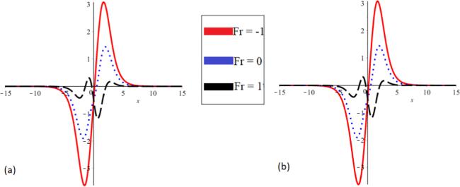
Now, by taking the YT of both sides of problem (31 ), we get:43 ), we have46 ) and the Adomian polynomials for nonlinear term as given in equation (25 ). Hence, solution (44 ), simplifies to50 ) and (51 ) into the following form solution40 ) and (52 ) derived using the HPTM and YTDM, respectively, to clearly illustrate and understand the effect of different physical and fractional parameters on their behavior. For the integer case $\left(\gamma =1\right)$, the two approximations (40 ) and (52 ) are graphically analyzed as illustrated in figures 1(a) and (b), respectively. Moreover, at $\left({{ \mathcal F }}_{r},n\right)=\left(-1,2\right)$, the two approximations (40 ) and (52 ) are compared with each other at different values for the fractional parameter γ as illustrated in figures 2(a) and (b), respectively. This comparative study highlights the sensitivity of the models to different values of fractional parameter γ, providing insights into the optimal conditions for each model's performance. Moreover, the two approximation (40 ) and (52 ) at $\left({F}_{r},n\right)=\left(-1,4\right)$ and for the integer case (γ = 1) are numerically investigated as illustrated in figures 3(a) and (b), respectively. Also, at $\left({F}_{r},n\right)=\left(-1,4\right)$, the impact of the fractional parameter γ on the two approximations (40 ) and (52 ) are numerically examined as evident in figures 4(a) and (b), respectively. Furthermore, the numerical investigation of the two approximations (40 ) and (52 ) for the integer case (γ = 1) and for $\left({F}_{r},n\right)=\left(-1,8\right)$ is depicted in figures 5(a) and (b), respectively. Additionally, the numerical analysis of the effect of the fractional parameter γ on the two approximations (40 ) and (52 ) is conducted at $\left({F}_{r},n\right)=\left(-1,8\right)$, as seen in figures 6(a) and (b), respectively. The results highlight the effect of the fractional parameter on the profile of the SWs, which contributes significantly to understanding the behavior of these waves. For $\left(\gamma ,n\right)=\left(1,8\right)$, the impact of Froude number Fr on the SW profile according to both HPTM and YTDM are examined as illustrated in figures 7(a) and (b), respectively.
$\begin{eqnarray}\begin{array}{l}{\bf{Y}}\left\{{D}_{T}^{\gamma }{\rm{\Phi }}\right\}=-c{\bf{Y}}\left\{\left[\left(({{ \mathcal F }}_{r}-1)-\displaystyle \frac{3}{2}\displaystyle \frac{{\rm{\Phi }}}{h}\right){\partial }_{X}{\rm{\Phi }}\right.\right.\\ \quad \left.\left.-\,\displaystyle \frac{1}{6}{h}^{2}{\partial }_{X}^{3}{\rm{\Phi }}+\displaystyle \frac{1}{2}{\partial }_{X}\left(1+0.1{{\rm{e}}}^{-\tfrac{{X}^{n}}{4}}\right)\right]\right\},\end{array}\end{eqnarray}$
which leads to $\begin{eqnarray}\begin{array}{l}\displaystyle \frac{1}{{u}^{\gamma }}\{M(u)-u{\rm{\Phi }}(0)\}=-c{\bf{Y}}\left\{\left[\left(({{ \mathcal F }}_{r}-1)-\displaystyle \frac{3}{2}\displaystyle \frac{{\rm{\Phi }}}{h}\right){\partial }_{X}{\rm{\Phi }}\right.\right.\\ \quad \left.\left.-\,\displaystyle \frac{1}{6}{h}^{2}{\partial }_{X}^{3}{\rm{\Phi }}+\displaystyle \frac{1}{2}{\partial }_{X}\left(1+0.1{{\rm{e}}}^{-\tfrac{{X}^{n}}{4}}\right)\right]\right\},\end{array}\end{eqnarray}$
and finally, we get $\begin{eqnarray}\begin{array}{l}M(u)=u{\rm{\Phi }}(0)-{{cu}}^{\gamma }{\bf{Y}}\left\{\left[\left(({{ \mathcal F }}_{r}-1)-\displaystyle \frac{3}{2}\displaystyle \frac{{\rm{\Phi }}}{h}\right){\partial }_{X}{\rm{\Phi }}\right.\right.\\ \quad \left.\left.-\,\displaystyle \frac{1}{6}{h}^{2}{\partial }_{X}^{3}{\rm{\Phi }}+\displaystyle \frac{1}{2}{\partial }_{X}\left(1+0.1{{\rm{e}}}^{-\tfrac{{X}^{n}}{4}}\right)\right]\right\}.\end{array}\end{eqnarray}$
Implementing the inverse YT for both sides of problem ( $\begin{eqnarray}\begin{array}{l}{\rm{\Phi }}={\rm{\Phi }}(0)-c{{\bf{Y}}}^{-1}\left[{u}^{\gamma }\left\{{\bf{Y}}\left(\left(({{ \mathcal F }}_{r}-1)-\displaystyle \frac{3}{2}\displaystyle \frac{{\rm{\Phi }}}{h}\right){\partial }_{X}{\rm{\Phi }}\right.\right.\right.\\ \quad -\,\displaystyle \frac{1}{6}{h}^{2}{\partial }_{X}^{3}{\rm{\Phi }}\\ \quad \left.\left.\left.+\,\displaystyle \frac{1}{2}{\partial }_{X}\left(1+0.1{{\rm{e}}}^{-\tfrac{{X}^{n}}{4}}\right)\right)\right\}\right],\end{array}\end{eqnarray}$
which equivalents μ $\begin{eqnarray}\begin{array}{l}{\rm{\Phi }}=-\displaystyle \frac{2{{\rm{e}}}^{X}}{{\left(1+{{\rm{e}}}^{X}\right)}^{2}}-c{{\bf{Y}}}^{-1}\left[{u}^{\gamma }\left\{{\bf{Y}}\left(\left(({{ \mathcal F }}_{r}-1)-\displaystyle \frac{3}{2}\displaystyle \frac{{\rm{\Phi }}}{h}\right){\partial }_{X}{\rm{\Phi }}\right.\right.\right.\\ \quad \left.\left.\left.-\,\displaystyle \frac{1}{6}{h}^{2}{\partial }_{X}^{3}{\rm{\Phi }}+\displaystyle \frac{1}{2}{\partial }_{X}\left(1+0.1{{\rm{e}}}^{-\tfrac{{X}^{n}}{4}}\right)\right)\right\}\right].\end{array}\end{eqnarray}$
The solution by means of infinite sequence reads $\begin{eqnarray}{\rm{\Phi }}\left(X,T\right)=\displaystyle \sum _{m=0}^{\infty }{{\rm{\Phi }}}_{m}(X,T).\end{eqnarray}$
By using equation ( $\begin{eqnarray}\begin{array}{l}\displaystyle \sum _{m=0}^{\infty }{{\rm{\Phi }}}_{m}(X,T)={\rm{\Phi }}(0)-c{{\bf{Y}}}^{-1}\\ \quad \times \,\left[{u}^{\gamma }\left\{{\bf{Y}}\left(\left(({{ \mathcal F }}_{r}-1){\partial }_{X}{\rm{\Phi }}\right)\displaystyle \frac{3}{2h}\displaystyle \sum _{m=0}^{\infty }{{ \mathcal A }}_{m}-\displaystyle \frac{1}{6}{h}^{2}{\partial }_{X}^{3}{\rm{\Phi }}\right.\right.\right.\\ \quad \left.\left.\left.+\,\displaystyle \frac{1}{2}{\partial }_{X}\left(1+0.1{{\rm{e}}}^{-\tfrac{{X}^{n}}{4}}\right)\right)\right\}\right],\end{array}\end{eqnarray}$
which equivalents $\begin{eqnarray}\begin{array}{l}\displaystyle \sum _{m=0}^{\infty }{{\rm{\Phi }}}_{m}(X,T)=-\displaystyle \frac{2{{\rm{e}}}^{X}}{{\left(1+{{\rm{e}}}^{X}\right)}^{2}}-c{{\bf{Y}}}^{-1}\\ \quad \times \left[{u}^{\gamma }\left\{{\bf{Y}}\left(\left(({{ \mathcal F }}_{r}-1){\partial }_{X}{\rm{\Phi }}\right)\displaystyle \frac{3}{2h}\displaystyle \sum _{m=0}^{\infty }{{ \mathcal A }}_{m}\right.\right.\right.\\ \quad \left.\left.\left.-\,\displaystyle \frac{1}{6}{h}^{2}{\partial }_{X}^{3}{\rm{\Phi }}+\displaystyle \frac{1}{2}{\partial }_{X}\left(1+0.1{{\rm{e}}}^{-\tfrac{{X}^{n}}{4}}\right)\right)\right\}\right].\end{array}\end{eqnarray}$
Some nonlinear terms are presented as follows: $\begin{eqnarray}\begin{array}{l}{H}_{0}({\rm{\Phi }})={{\rm{\Phi }}}_{0}{\left({{\rm{\Phi }}}_{0}\right)}_{X},\\ {H}_{1}({\rm{\Phi }})={{\rm{\Phi }}}_{1}{\left({{\rm{\Phi }}}_{0}\right)}_{X}+{{\rm{\Phi }}}_{0}{\left({{\rm{\Phi }}}_{1}\right)}_{X},\\ \vdots \end{array}\end{eqnarray}$
By matching either sides of the above equation, we get $\begin{eqnarray}{{\rm{\Phi }}}_{0}(X,T)=-\frac{2{{\rm{e}}}^{X}}{{\left(1+{{\rm{e}}}^{X}\right)}^{2}},\end{eqnarray}$
for m = 0, and for m = 1, we have $\begin{eqnarray}\begin{array}{c}{{\rm{\Phi }}}_{1}(X,T)=-\frac{{T}^{\gamma }c}{{\rm{\Gamma }}(\gamma +1)}\left[\frac{6{{\rm{e}}}^{2X}(-1+{{\rm{e}}}^{X})}{{\left(1+{{\rm{e}}}^{X}\right)}^{5}h}\right.\\ \quad -\,\frac{{{\rm{e}}}^{X}(-1+11{{\rm{e}}}^{X}-11{{\rm{e}}}^{2X}+{{\rm{e}}}^{3X}){h}^{2}}{3{\left(1+{{\rm{e}}}^{X}\right)}^{5}}\\ \quad \left.-\,0.0125{{nX}}^{-1+n}{{\rm{e}}}^{-\tfrac{{X}^{n}}{4}}+\frac{2{{\rm{e}}}^{X}(-1+{{\rm{e}}}^{X})(-1+{{ \mathcal F }}_{r})}{{\left(-1+{{\rm{e}}}^{X}\right)}^{3}}\right].\end{array}\end{eqnarray}$
Finally, the YTDM approximation for (m ≥ 1) can be calculated in the same manner. Thus, the approximate solution until the second-order approximation can be obtained by inserting the values of Φ0(X, T) and Φ1(X, T) given, respectively, in equations ( $\begin{eqnarray}{\rm{\Phi }}(X,T)=\displaystyle \sum _{m=0}^{\infty }{{\rm{\Phi }}}_{m}(X,T)={{\rm{\Phi }}}_{0}(X,T)+{{\rm{\Phi }}}_{1}(X,T)+\cdots .\end{eqnarray}$
We perform a quantitative examination for solutions (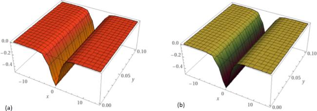
Figure 1. The two approximations ( |
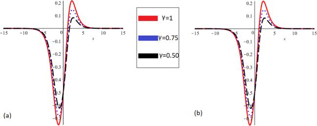
Figure 2. The behavior of the two approximations ( |
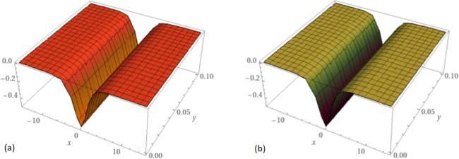
Figure 3. The two approximations ( |
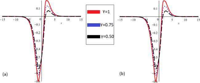
Figure 4. The behavior of the two approximations ( |
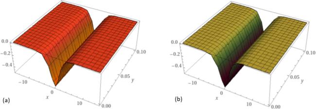
Figure 5. The two approximations ( |
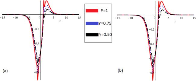
Figure 6. The behavior of the two approximations ( |
Figure 7. The behavior of the two approximations ( |
Ultimately, the derived approximations using both HPTM and YTDM approaches are characterized by high accuracy and stability at large study domain values. These methods are also characterized by simplicity and avoid many mathematical complications that may result from other methods. The obtained approximations also accurately describe the solitary waves and how the fractional parameter impacts their profile.
7. Conclusion
In this investigation, the fractional forced Korteweg–de Vries (FF-KdV) equation has been analyzed using YTDM and YHPM in the framework of Caputo operator. Two analytical approximations have been derived using the proposed techniques. The generated approximations have undergone numerical analysis using specific numerical values for the relevant parameters. The numerical analysis results exhibited a notable level of precision in the derived approximations. This was evident when comparing these approximations with the precise analytical solutions of the integer case and between these approximations themselves. Based on the recommended methodologies for addressing the stated issue, it has been verified that the mathematical model of fractional order exhibits superior accuracy in interpreting experimental data compared to the integer-order model.
The obtained results showcase the robustness of suggested techniques in terms of accuracy and their extensive range of applicability to problems involving fractional nonlinear dynamics. Therefore, these techniques can be utilized to examine diverse forms of nonlinear problems that inherently arise in real-world scenarios, especially to analyze many nonlinear evolution equations used to describe various nonlinear structures in different plasma models.
Future work: it is necessary to examine and analyze various fractional nonlinear evolution equations related to various plasma models to reveal the ambiguity around some phenomena that arise in different plasma models. For instance, the damped FF-KdV equation, nonplanar FF-KdV equation, damped nonplanar FF-KdV equation, and many other related equations with higher-order nonlinearity and dispersion should be investigated [37–44].
Acknowledgments
The authors express their gratitude to Princess Nourah bint Abdulrahman University Researchers Supporting Project number (PNURSP2024R229), Princess Nourah bint Abdulrahman University, Riyadh, Saudi Arabia.
Conflict of interest
The authors declare that they have no conflicts of interest.
Authors contributions
All authors contributed equally and approved the final version of the current manuscript.