


1. Introduction
The following (2+1)-dimensional generalization of the Korteweg–de Vries equation
$\begin{eqnarray}{w}_{{t}_{1}}+{w}_{{xxx}}-3{\left(w{{\rm{\partial }}}_{y}^{-1}{w}_{x}\right)}_{x}=0,\,{{\rm{\partial }}}_{y}^{-1}={\int }_{-\infty }^{y}\cdot \,{\rm{d}}{y},\end{eqnarray}$
known as Boiti–Leon–Manna–Pempinelli equation or asymmetric Nizhnik–Novikov–Veselov (ANNV) equation, was firstly derived by using the concept of the weak Lax pair [1]. The ANNV system is of great importance in the fields of incompressible fluid mechanics and acoustics [2]. In particular, it finds applications in various nonlinear phenomena, including shallow water waves characterized by weak nonlinear resilience, the propagation of longinternal waves in density stratified oceans, and the behavior of acoustic waves on lattices [3].In recent years, the ANNV system has been widely and profoundly studied [4–18]. Lou [4] confirmed that the system can also be derived from the internal parameter-dependent symmetry constraint of the Kadomtsev–Petviashvili equation. Fan utilized the multi-dimensional Riemann theta function to construct two-periodic wave solutions and conducted asymptotic analysis [5]. The study also rigorously demonstrated that the periodic wave solutions tend towards the soliton solutions under the small amplitude limit. Zhang derived two kinds of deformation rogue waves through the combination of a positive quadratic function and hyperbolic cosine function [6]. Guo constructed new kinds of rogue wave solutions doubly localized in time and space by using the binary Darboux transformation [7]. Zhao constructed the resonance Y-type soliton and interaction solutions by imposing additional constraints on the parameters of the N-soliton solutions [8]. Li introduced a novel method for solving the ANNV system based on the $\overline{\partial }$-dressing approach, emphasizing the key step of connecting characteristic functions and the $\overline{\partial }$-problem [9]. Furthermore, the variable separation solutions of the ANNV system have been extensively studied. Based on the system, the multilinear variable separation approach (MLVSA) was clearly proposed, confirming the existence of localized structures such as dromion solutions, lumps, breathers, instantons, and the ring-type soliton [10]. Dai obtained variable separation solutions by refining the extended tanh-function method, including lower-dimensional arbitrary functions in their exact solutions [11]. Kumar achieved trilinearization and identified localized coherent structures using the truncated Painlevé expansion method [12].
According to the formal series symmetry approach [19–21], the ANNV system possess a series of mastersymmetries and the following obvious time-independent symmetries4 ) can be rewritten in potential form
$\begin{eqnarray}{K}_{0}(w)={w}_{x},\quad {K}_{1}(w)=3{\left(w{\partial }_{y}^{-1}{w}_{x}\right)}_{x}-{w}_{{xxx}}.\end{eqnarray}$
We choose a suitable mastersymmetry of degree one [22] $\begin{eqnarray}\begin{array}{l}M=x{\left(w{\partial }_{y}^{-1}{w}_{x}\right)}_{x}-\displaystyle \frac{1}{3}({{xw}}_{{xxx}}+2{w}_{{xx}}\\ \quad -\,4w{\partial }_{y}^{-1}{w}_{x}-{w}_{x}{\partial }_{y}^{-1}w),\end{array}\end{eqnarray}$
and apply it to the time-independent symmetry K1, resulting in a fifth-order ANNV (FANNV) equation $\begin{eqnarray}\begin{array}{l}{w}_{{t}_{2}}=[M,{K}_{1}]=-{w}_{{xxxxx}}\\ \,-\,\left[\displaystyle \frac{15}{2}w{\left({\partial }_{y}^{-1}{w}_{x}\right)}^{2}+5w{\partial }_{y}^{-1}\right.\\ \quad {\left.\times \,(w{\partial }_{y}^{-1}{w}_{{xx}})-5w{\partial }_{y}^{-1}{w}_{{xxx}}-5{w}_{x}{\partial }_{y}^{-1}{w}_{{xx}}-5{w}_{{xx}}{\partial }_{y}^{-1}{w}_{x}\right]}_{x},\end{array}\end{eqnarray}$
where the Lie product [,] are defined as $\begin{eqnarray*}\begin{array}{l}[A(u),B(u)]=A^{\prime} B-{BA}^{\prime} =\displaystyle \frac{\partial }{\partial \epsilon }[A(u+\epsilon B(u))\\ \quad {\left.-\,B(u+\epsilon A(u))]\right|}_{\epsilon =0}.\end{array}\end{eqnarray*}$
After rescaling t2 → t and setting w = ux = vy, equation ( $\begin{eqnarray}\begin{array}{l}({u}_{{xy}}-{u}_{x}{\partial }_{y})\left[{u}_{t}+{u}_{{xxxxx}}-5{\left({u}_{{xx}}{v}_{x}\right)}_{x}\right]\\ \quad +\,5{u}_{x}^{2}({v}_{{xxxy}}-3{v}_{x}{v}_{{xy}})-5{u}_{x}^{3}{v}_{{xx}}=0,\\ \quad {u}_{x}-{v}_{y}=0.\end{array}\end{eqnarray}$
In this paper we deal with the variable separation solution of the potential FANNV system (5 ). The paper is organized as follows: the second section focuses on obtaining variable separation solutions based on a hexagonal linear equation. Following this, the third section introduces several novel patterns of localized excitations. In the fourth section, we present solitary wave solutions of the fusion or fission type and provide illustrative examples. Finally, the paper concludes with a discussion of the results.
2. Variable separation solution
To construct exact solutions of the potential FANNV system (5 ), we take the truncated Laurent series at the constant level term6 ) into (5 ) results in the following hexagonal linear equation7 ) degenerates into a trilinear equation:9 ) into the equation (8 ), we obtain:7 ) into a (1+1)-dimensional bilinear equation of q. The general solution to equation (10 ) is:9 ) and (11 ) into (6 ) gives the variable separation solutions of the potential FANNV system
$\begin{eqnarray}u=-2{\left(\mathrm{ln}f\right)}_{y}+{u}_{0},\quad v=-2{\left(\mathrm{ln}f\right)}_{x}+{v}_{0},\end{eqnarray}$
where f is an undetermined function of (x, y, t), u0 and v0 are seed solutions satisfying the potential FANNV system. With the special choice of the seed solution u0 = 0 and v0 = 0, the substitution of ( $\begin{eqnarray}\begin{array}{l}\displaystyle \frac{10{f}_{x}^{3}({f}_{2x}h-{f}_{x}{h}_{x})}{{f}^{6}}-\displaystyle \frac{10{f}_{x}^{2}({f}_{3x}h-{f}_{x}{h}_{{xx}})}{{f}^{5}}\\ \quad +\,\displaystyle \frac{5{f}_{x}({f}_{4x}h-{f}_{x}{h}_{{xxx}})}{{f}^{4}}\\ \quad -\,\displaystyle \frac{{hg}+{f}_{x}({f}_{{yy}}{g}_{y}-{f}_{y}{g}_{{yy}})+5{f}_{x}({f}_{{xyy}}{f}_{4{xy}}-{f}_{{xy}}{f}_{4{xyy}})}{{f}^{3}}\\ \quad +\,\displaystyle \frac{{f}_{{xyy}}{g}_{y}-{f}_{{xy}}{g}_{{yy}}}{{f}^{2}}=0,\quad h={f}_{y}{f}_{{xyy}}-{f}_{{xy}}{f}_{{yy}},\\ \quad g={f}_{t}+{f}_{5x},\quad {f}_{{mx}}=\displaystyle \frac{{{\rm{d}}}^{m}f}{{\rm{d}}{x}^{m}}.\end{array}\end{eqnarray}$
We introduce the constraint h = fyfxyy − fxyfyy = 0 to ensure that the coefficients of (f−6, f−5, f−4) are zero. Then, equation ( $\begin{eqnarray}\begin{array}{l}f({f}_{{xyy}}{g}_{y}-{f}_{{xy}}{g}_{{yy}})-{f}_{x}({f}_{{yy}}{g}_{y}-{f}_{y}{g}_{{yy}})\\ \quad -\,5{f}_{x}({f}_{{xyy}}{f}_{4{xy}}-{f}_{{xy}}{f}_{4{xyy}})=0.\end{array}\end{eqnarray}$
Given h = 0, f can be solved as follows $\begin{eqnarray}f={p}_{1}+{p}_{2}q,\end{eqnarray}$
where p1 = p1(x, t), p2 = p2(x, t), and q = q(y, t) are functions of indicated variables. Notably, the variables x and y are completely separated into p1 = p1(x, t), p2 = p2(x, t), and q = q(y, t), respectively. Substituting equation ( $\begin{eqnarray}{q}_{{yt}}{q}_{{yy}}-{q}_{{yyt}}{q}_{y}=0.\end{eqnarray}$
Now, the solution problem is reformulated from a (2+1)-dimensional hexagonal linear equation ( $\begin{eqnarray}q={YT}+{T}_{1},\end{eqnarray}$
where Y = Y(y), T = T(t) and T1 = T1(t). Finally, substituting ( $\begin{eqnarray}u=-\displaystyle \frac{2{p}_{2}{Y}_{y}T}{{p}_{1}+{p}_{2}({YT}+{T}_{1})},\quad v=-\displaystyle \frac{2{p}_{1x}+2{p}_{2x}({YT}+{T}_{1})}{{p}_{1}+{p}_{2}({YT}+{T}_{1})}.\end{eqnarray}$
The expression of u and v indicates the possibility of exploring local excitations for the physical quantity $\begin{eqnarray}\begin{array}{l}w={u}_{x}={v}_{y}=-\displaystyle \frac{2({p}_{1}{p}_{2x}-{p}_{1x}{p}_{2}){q}_{y}}{{\left({p}_{1}+{p}_{2}q\right)}^{2}}\\ \quad =\,-\displaystyle \frac{2({p}_{1}{p}_{2x}-{p}_{1x}{p}_{2}){Y}_{y}T}{{\left[{p}_{1}+{p}_{2}({YT}+{T}_{1})\right]}^{2}}.\end{array}\end{eqnarray}$
Under the constraints p1 = a0 + a1p and p2 = a2 + a3p, it is interesting that the physical field w takes the form of the so-called universal quantity valid for a large class of multilinear variable separable systems [23, 24]: $\begin{eqnarray*}\begin{array}{l}w=\displaystyle \frac{2{A}_{0}{p}_{x}{q}_{y}}{{\left({a}_{0}+{a}_{1}p+{a}_{2}q+{a}_{3}{pq}\right)}^{2}},\\ \quad {A}_{0}={a}_{0}{a}_{3}-{a}_{1}{a}_{2}.\end{array}\end{eqnarray*}$
3. New patterns of the localized excitations
Take13 ) becomes16 ) into (15 ), the function describing the variation of amplitude with time can be derived
$\begin{eqnarray}\begin{array}{l}{p}_{1}={a}_{0}+{a}_{1}{{\rm{e}}}^{{\xi }_{1}},\quad {p}_{2}={a}_{2}+{a}_{3}{{\rm{e}}}^{{\xi }_{1}},\\ Y=1+{{\rm{e}}}^{\eta },\quad {T}_{1}=0,\\ {\xi }_{1}={k}_{1}x+{\omega }_{1}t+{x}_{10},\quad \eta ={l}_{1}y+{y}_{10},\end{array}\end{eqnarray}$
the solution ( $\begin{eqnarray}w=-\displaystyle \frac{2{k}_{1}{l}_{1}{A}_{0}T{{\rm{e}}}^{{\xi }_{1}+\eta }}{{\left[{a}_{0}+{a}_{1}{{\rm{e}}}^{{\xi }_{1}}+T({a}_{2}+{a}_{3}{{\rm{e}}}^{{\xi }_{1}})(1+{{\rm{e}}}^{\eta })\right]}^{2}}.\end{eqnarray}$
Given that ${a}_{3}\gt \left|{a}_{1}\right|\gt 0$, ${a}_{2}\gt \left|{a}_{0}\right|\gt 0$, and that T is equal to 1, the solution describes a dromion moving along a straight line parallel to the x-axis. This fact prompts us to consider a question: when the function T displays a specific asymptotic behavior, does the dromion structure exhibit a similar one? Let wx = wy = 0, the trajectory of the crest of the dromion can be described by the following parametric equations $\begin{eqnarray}\begin{array}{rcl}{\xi }_{1} & = & {k}_{1}x+{\omega }_{1}t+{x}_{10}=\mathrm{ln}(\beta ),\\ \eta & = & \mathrm{ln}\left\{\displaystyle \frac{({a}_{0}+{a}_{2}T)}{{a}_{3}\beta T}\right\},\\ \beta & = & \beta (t)={\left[\displaystyle \frac{{a}_{2}({a}_{0}+{a}_{2}T)}{{a}_{3}({a}_{1}+{a}_{3}T)}\right]}^{\tfrac{1}{2}}.\end{array}\end{eqnarray}$
Substituting ( $\begin{eqnarray}A=\displaystyle \frac{2{a}_{3}{k}_{1}{l}_{1}{A}_{0}({a}_{0}+{a}_{2}T){\beta }^{2}}{{\left[{a}_{0}{a}_{2}+2{a}_{0}{a}_{3}\beta +{a}_{1}{a}_{3}{\beta }^{2}+{\left({a}_{2}+{a}_{3}\beta \right)}^{2}T\right]}^{2}}.\end{eqnarray}$
In the following, we will examine the dynamical behavior of u with different choices of the function T.
3.1. Dromioff: a temporal kink
As the first case, we consider T = eΩt. In this case, w can be expressed as16 ) for the trajectory of the dromion crest becomes19 ) into (18 ) results in the amplitude of the dromion
$\begin{eqnarray}w=-\displaystyle \frac{2{k}_{1}{l}_{1}{A}_{0}{{\rm{e}}}^{{\xi }_{1}+\eta +{\rm{\Omega }}t}}{{\left[{a}_{0}+{a}_{1}{{\rm{e}}}^{{\xi }_{1}}+{{\rm{e}}}^{{\rm{\Omega }}t}({a}_{2}+{a}_{3}{{\rm{e}}}^{{\xi }_{1}})(1+{{\rm{e}}}^{\eta })\right]}^{2}},\end{eqnarray}$
and parametric equations ( $\begin{eqnarray}\begin{array}{rcl}{\xi }_{1} & = & {k}_{1}x+{\omega }_{1}t+{x}_{10}=\mathrm{ln}({\beta }_{1}),\\ {\eta }^{{\prime} } & = & \eta +{\rm{\Omega }}t=\displaystyle \frac{{a}_{0}+{a}_{2}{{\rm{e}}}^{{\rm{\Omega }}t}}{{a}_{3}\mathrm{ln}({\beta }_{1})},\\ {\beta }_{1} & = & {\beta }_{1}(t)={\left[\displaystyle \frac{{a}_{2}({a}_{0}+{a}_{2}{{\rm{e}}}^{{\rm{\Omega }}t})}{{a}_{3}({a}_{1}+{a}_{3}{{\rm{e}}}^{{\rm{\Omega }}t})}\right]}^{\tfrac{1}{2}}.\end{array}\end{eqnarray}$
Substitution of ( $\begin{eqnarray}\begin{array}{rcl}A & = & -\displaystyle \frac{{a}_{2}{k}_{1}{l}_{1}{A}_{0}}{2({a}_{1}+{a}_{3}{{\rm{e}}}^{{\rm{\Omega }}t}){\left[{a}_{2}+{a}_{3}\mathrm{ln}({\beta }_{1})\right]}^{2}},\\ {A}_{\max } & = & \displaystyle \frac{{k}_{1}{l}_{1}}{2{A}_{0}}{\left(\sqrt{{a}_{0}{a}_{3}}-\sqrt{{a}_{1}{a}_{2}}\right)}^{2}.\end{array}\end{eqnarray}$
With Ω > 0 and t → − ∞ , the limiting values of ξ and ${\eta }^{{\prime} }$ can be calculated as21 ), we can derive an equation for the trajectory in terms of x and y22 ), both ξ1 and ${\eta }^{{\prime} }$ are constants. It can be inferred that the limit of w corresponds to a standard dromion structure19 ) degenerate to ${\xi }_{1}=\mathrm{ln}({a}_{2}/{a}_{3})$ and η = 0. In this case, the dromion moves along a straight line parallel to the x axis at a constant velocity. It is obvious that the limits of f and w are
$\begin{eqnarray}{\xi }_{1}=\displaystyle \frac{1}{2}\mathrm{ln}\left(\displaystyle \frac{{a}_{0}{a}_{2}}{{a}_{1}{a}_{3}}\right),\quad {\eta }^{{\prime} }=\displaystyle \frac{1}{2}\mathrm{ln}\left(\displaystyle \frac{{a}_{0}{a}_{1}}{{a}_{2}{a}_{3}}\right).\end{eqnarray}$
By eliminating t from equation ( $\begin{eqnarray}y=\displaystyle \frac{{\rm{\Omega }}}{{k}_{1}{l}_{1}}\left[{k}_{1}x+{x}_{10}+\displaystyle \frac{1}{2}\mathrm{ln}\left(\displaystyle \frac{{a}_{1}{a}_{3}}{{a}_{0}{a}_{2}}\right)\right]+\displaystyle \frac{1}{2{l}_{1}}\mathrm{ln}\left(\displaystyle \frac{{a}_{0}{a}_{1}}{{a}_{2}{a}_{3}}\right).\end{eqnarray}$
When the dromion moves along the straight line ( $\begin{eqnarray}w\left|{}_{t\to -\infty }\right.=\displaystyle \frac{2{k}_{1}{l}_{1}{A}_{0}{{\rm{e}}}^{{\xi }_{1}+{\eta }^{{\prime} }}}{{\left({a}_{0}+{a}_{1}{{\rm{e}}}^{{\xi }_{1}}+{a}_{2}{{\rm{e}}}^{{\eta }^{{\prime} }}+{a}_{3}{{\rm{e}}}^{{\xi }_{1}+{\eta }^{{\prime} }}\right)}^{2}}.\end{eqnarray}$
As t → + ∞ , parametric equations ( $\begin{eqnarray}f\left|{}_{t\to +\infty }\right.={a}_{0}+{a}_{1}{{\rm{e}}}^{{\xi }_{1}},\quad w\left|{}_{t\to +\infty }\right.=0\end{eqnarray}$
Based on the asymptotic analysis, it is clear that the dromion only appears as t → −∞ when Ω > 0, while it exclusively manifests as t → + ∞ when Ω < 0. Similar to the definition of solitoff [25], a deactivated line soliton on a half-space line, a ‘dromioff' is defined as a deactivated dromion on the half-time line. Comparing figures 1(a)–(b), where time ranges from t = −55 to t = −15, no significant amplitude change of the dromion can be observed. In contrast, figures 1(b)–(d) indicate a rapid transition in amplitude near t = 0. In figure 1(d), the amplitude becomes imperceptible, indicating an approximate decrease to 5 × 10⁻³ at this point. Figure 2(a) depicts the temporal evolution of amplitude over time. The figure clearly illustrates that an increased value of Ω results in a more significant amplitude variation. The temporal evolution of the amplitude has a kink shape and can be referred to as a temporal kink. Figures 2(b) presents the track of the dromioff. As t approaches −∞ , the trajectory approximates y = 0.5x, and as t approaches + ∞ , the trajectory approximates y = 0.
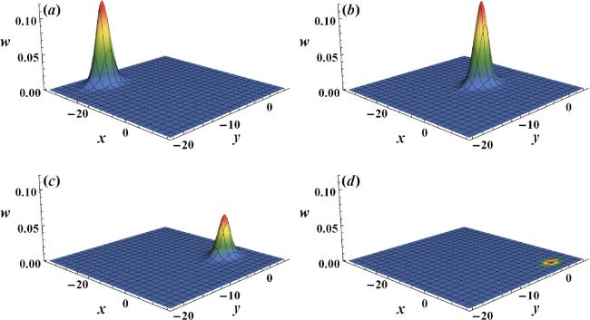
Figure 1. Space-time evolution of a dromioff solution ( |
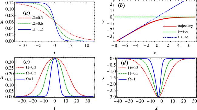
Figure 2. Amplitude and trajectory curves. (a) Variation of dromioff amplitude with respect to t under different Ω values. The parameter settings are k1 = a1 = a2 = 1, l1 = −1.2, ω1 = −0.5, a0 = a3 = 1.5, and x10 = y10 = 0. (b) The corresponding trajectory of dromioff with Ω = 0.3. (c) Variation of amplitude of the dromion-type instanton with different Ω values. The parameter are k1 = 1, l1 = ω1 = –1, a0 = a3 = 10, a1 = 30, a2 = 0.1, and x10 = y10 = 0. (d) The corresponding trajectory of dromion-type instanton. |
3.2. Instanton moving along the curved line
In the second case, we consider $T=\cosh (\omega t)$. In this scenario, w can be expressed in terms of16 ) for the trajectory can be rewritten as26 ) becomes ${\xi }_{1}=\mathrm{ln}\left({a}_{2}/{a}_{3}\right)$ and η = 0, indicating that the dromion moves along the line y = −y10/l1, and it is evident that the limits of f and w are27 ) suggests that the dromion structure emerges solely near t = 0 and disappears as time t approaches ±∞. This asymptotic pattern aligns with the definition of instantons in quantum chromodynamics, and we refer to it as a dromion-type instanton. Figure 3 illustrates the spatiotemporal evolution of the instanton. The figures demonstrate that the instanton described in (25 ) reaches its maximum amplitude at at t = 0 and then exponentially decays as t → ±∞. In figure 3(e), the amplitude becomes imperceptible, decreasing to approximately 10−3. By substituting equations (26 ) into (25 ), we can determine the amplitude of the dromion-type instanton
$\begin{eqnarray}w=-\displaystyle \frac{2{k}_{1}{l}_{1}{A}_{0}{{\rm{e}}}^{{\xi }_{1}+\eta }\cosh ({\rm{\Omega }}t)}{{\left[{a}_{0}+{a}_{1}{{\rm{e}}}^{{\xi }_{1}}+\cosh ({\rm{\Omega }}t)({a}_{2}+{a}_{3}{{\rm{e}}}^{{\xi }_{1}})(1+{{\rm{e}}}^{\eta })\right]}^{2}},\end{eqnarray}$
and parametric equation ( $\begin{eqnarray}\begin{array}{rcl}{\xi }_{1} & = & {k}_{1}x+{\omega }_{1}t+{x}_{10}=\mathrm{ln}({\beta }_{2}),\\ \eta & = & {l}_{1}y+{y}_{10}=\displaystyle \frac{{a}_{2}+{a}_{0}{\rm{sech}} ({\rm{\Omega }}t)}{{a}_{3}\mathrm{ln}({\beta }_{2})},\\ {\beta }_{2} & = & {\beta }_{2}(t)={\left[\displaystyle \frac{{a}_{2}({a}_{2}+{a}_{0}{\rm{sech}} ({\rm{\Omega }}t)}{{a}_{3}({a}_{3}+{a}_{1}{\rm{sech}} ({\rm{\Omega }}t)}\right]}^{\tfrac{1}{2}}.\end{array}\end{eqnarray}$
As t → ±∞, equation ( $\begin{eqnarray}f\left|{}_{t\to \pm \infty }\right.=({a}_{2}+{a}_{3}{{\rm{e}}}^{{\xi }_{1}})(1+{{\rm{e}}}^{\eta }),\quad w\left|{}_{t\to \pm \infty }\right.=0.\end{eqnarray}$
Equation ( $\begin{eqnarray}A=-\displaystyle \frac{{a}_{2}{k}_{1}{l}_{1}{A}_{0}}{2({a}_{1}+{a}_{3}\cosh ({\rm{\Omega }}t){\left[{a}_{2}+{a}_{3}\mathrm{ln}({\beta }_{2})\right]}^{2}}.\end{eqnarray}$
Figure 2(c) presents the variation curve of the amplitude with respect to t, indicating that the dromion-type instanton is also localized in time. From the figure, it can be observed that the larger the value of Ω, the more pronounced the amplitude variation. Figure 2(d) illustrates the trajectory of the dromion-type instanton. As t → ±∞, the trajectory can be approximated as y = 0, while around t = 0, the trajectory exhibits a bell-shaped profile.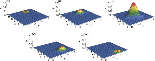
Figure 3. Space-time evolution of the instanton solution ( |
3.3. Tempo-spatial breather
As the third case, we adopt T as the Jacobi elliptic function:17 ), the dromion reaches its peak at cn=0 and its minimum amplitude at cn=1. Figure 4(e) shows the trajectory curve as described by equation (16 ), indicating the breather-like motion of the dromion along the periodic trajectory.
$\begin{eqnarray}T={b}_{0}+{b}_{1}{cn}({\rm{\Omega }}t,m).\end{eqnarray}$
By introducing the periodic function T, the identity of the dromion shows periodic variations in both space and time scales. Consequently, it is termed a tempo-spatial breather. Figure 4 shows the spatio-temporal evolution of the dromion in a three-dimensional plot, the amplitude curve and the trajectory with the following parameter settings $\begin{eqnarray}\begin{array}{rcl}{k}_{1} & = & {l}_{1}={a}_{2}=-{\omega }_{1}={\rm{\Omega }}=1,\\ {a}_{0} & = & {a}_{3}=3,\quad {a}_{1}={b}_{1}=30,\quad {b}_{0}=0.1,\\ m & = & 0.999,\quad {x}_{10}={y}_{10}=0.\end{array}\end{eqnarray}$
In figure 4(d), the periodic curve describing the amplitude variation over time is presented. As can be inferred from equation (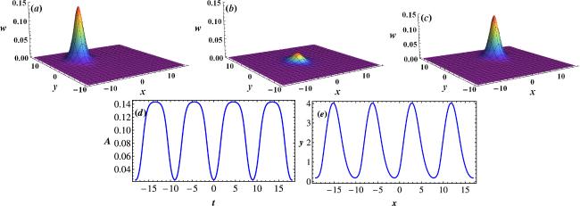
Figure 4. Plots illustrating the tempo-spatial breather. (a) 3D plot at t = –3.35; (b) 3D plot at t = 0; (c) 3D plot at t = 3.35; (d) Amplitude variations with respect to t; (e) Trajectory curves. |
4. Fusion or fission type solitary wave solution
If p1 and p2 are selected as
$\begin{eqnarray}\begin{array}{rcl}{p}_{1} & = & \displaystyle \sum _{i=1}^{M}{{\rm{e}}}^{{\xi }_{i}},\quad {p}_{2}=\displaystyle \sum _{j=1}^{N}{{\rm{e}}}^{{\zeta }_{j}},\\ {\xi }_{i} & = & {k}_{i}x+{\omega }_{i}t+{\xi }_{i0},\quad {\zeta }_{j}={K}_{j}x+{{\rm{\Omega }}}_{j}t+{\zeta }_{j0},\end{array}\end{eqnarray}$
where M and N are arbitrary positive integers, one obtain the fusion or fission type solitary waves solution [26]. Below are some interesting examples.As a first example, the fission phenomenon between a solitoff and a dromion can be observed by taking
$\begin{eqnarray}\begin{array}{rcl}{p}_{1} & = & 1+{{\rm{e}}}^{0.9x-0.6t},\,{p}_{2}=1+{{\rm{e}}}^{-0.6x-0.08t},\\ Y & = & 1+{{\rm{e}}}^{0.6y},\,T=1,\,{T}_{1}=0.\end{array}\end{eqnarray}$
Figure 5 depicts the completely inelastic interaction between the two waves. In figure 5(a), a solitoff with a peak at the front is observable. Moving to figure 5(b), the peak of the solitoff vanishes, and the front bottom becomes flat. Figure 5(c) shows the fission of a resonant solitoff into a solitoff and a dromion.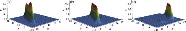
Figure 5. The scenario of a completely inelastic collision between a soliton and a dromion with p1, p2 and q given in ( |
As a second illustration, an intriguing phenomenon appears that is similar to an instanton, as shown in figure 6 by the setting of
$\begin{eqnarray}\begin{array}{rcl}{p}_{1} & = & {{\rm{e}}}^{1.5x+8t}+{{\rm{e}}}^{-0.9x+0.6t}+{{\rm{e}}}^{0.3x-0.003t},\quad {p}_{2}=1,\\ Y & = & \displaystyle \frac{3+{{\rm{e}}}^{-y}}{1+3{{\rm{e}}}^{-y}},\quad T=1,\quad {T}_{1}=0.\end{array}\end{eqnarray}$
Figure 6 presents the spatiotemporal evolution diagram of the instanton excited by three-resonant dromions. In figure 6(a), only a small dipole-dromion is observable. The amplitudes of the dipole-dromion progressively increase in figures 6(a)–(c), reaching its maximum at t = 0. In figure 6(d), the amplitude of the dromion noticeably decreases, and the superposition of a third dromion on the bright dromion becomes visible. By t = 10 in figure 6(e), the amplitude has descended to 3.9 × 10⁻². Figure 6(f) provides cross-sectional images at different times for y = 0.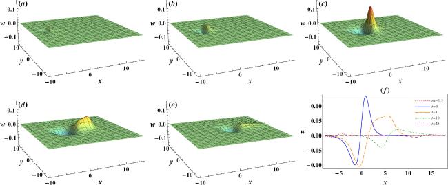
Figure 6. Spacetime evolution of the instanton-like excitation with p1, p2 and q given in equation ( |
As a last scenario we take
$\begin{eqnarray}\begin{array}{rcl}{p}_{1} & = & 1+{{\rm{e}}}^{0.9x-0.6t},\quad {p}_{2}=1+{{\rm{e}}}^{-0.6x+0.08t},\\ Y & = & \displaystyle \frac{3+{{\rm{e}}}^{-1.2y}}{1+3{{\rm{e}}}^{-1.2y}},\quad T={{\rm{e}}}^{0.1t},\quad {T}_{1}=0,\end{array}\end{eqnarray}$
to illustrate the completely inelastic interaction between a dromion and a dromioff. In figure 7(a) only a tall and slender dromion is visible, while in figure 7(b) the dromion shortens and shows a flattened base. Next, in figure 7(c), the dromion undergoes fission, resulting in the formation of a dromion and a dromioff, with the amplitude of the latter decaying exponentially. Finally, in figure 7(d), the amplitude of the dromioff decreases significantly.
Figure 7. Completely inelastic interaction between a dromion and a dromioff with p1, p2 and q given in ( |
5. Conclusions and discussions
In summary, variable separation solutions for the FANNV equation are obtained using the truncated Painlevé expansion with a specific selection of the seed solution. These solutions lead to the construction of new patterns of localized excitations. In particular, a new nonlinear excitation called dromioff is introduced, which represents a deactivated dromion positioned along the half-time line. However, the mechanism underlying the excitation of the dromioff needs further consideration.