


1. Introduction
2. Cosmic string effect on the solution of the Schrödinger equation with extended ring-shaped potential
2.1. Numerical examples of the eigenvalue solution
| i | (i) For m = 0 is Θ0(θ) ≡ 1 with the constraints: $\begin{eqnarray}\left\{\begin{array}{l}{\lambda }_{{\ell },0}=\displaystyle \frac{{{\ell }}^{2}}{{\alpha }^{2}};\\ {b}_{8}=1;\\ {b}_{7}=-\displaystyle \frac{{{\ell }}^{2}}{2{\alpha }^{2}}.\end{array}\right.\end{eqnarray}$ |
| ii | (ii) For m = 1, we have ${x}_{1}=\pm \displaystyle \frac{\sqrt{2}}{2}$ then we get: |
| • | ${{\rm{\Theta }}}_{1}(\theta )=\sin \theta +\displaystyle \frac{\sqrt{2}}{2},$ for ${x}_{1}=-\displaystyle \frac{\sqrt{2}}{2}$, the constraints are, $\begin{eqnarray}\left\{\begin{array}{l}{\lambda }_{{\ell },1}=2+\displaystyle \frac{{{\ell }}^{2}}{{\alpha }^{2}};\\ {b}_{8}=1+\displaystyle \frac{1}{\sqrt{2}};\\ {b}_{7}=-\displaystyle \frac{{{\ell }}^{2}}{2{\alpha }^{2}}.\end{array}\right.\end{eqnarray}$ |
| • | ${{\rm{\Theta }}}_{1}(\theta )=\sin \theta -\displaystyle \frac{\sqrt{2}}{2},$ for ${x}_{1}=\displaystyle \frac{\sqrt{2}}{2}$ and the conditions are, $\begin{eqnarray}\left\{\begin{array}{l}{\lambda }_{{\ell },1}=2+\displaystyle \frac{{{\ell }}^{2}}{{\alpha }^{2}};\\ {b}_{8}=1-\displaystyle \frac{1}{\sqrt{2}};\\ {b}_{7}=-\displaystyle \frac{{{\ell }}^{2}}{2{\alpha }^{2}}.\end{array}\right.\end{eqnarray}$ |
| i | (iii) For m = 2 $\begin{eqnarray}{{\rm{\Theta }}}_{2}(x)=(x-{x}_{1})(x-{x}_{2}),\end{eqnarray}$ where the roots x1 , x2 satisfy the following Bethe ansatz equations: $\begin{eqnarray}\displaystyle \frac{2}{{x}_{1}-{x}_{2}}+\displaystyle \frac{2{x}_{1}^{2}-1}{{x}_{1}\left({x}_{1}^{2}-1\right)}=0,\end{eqnarray}$ $\begin{eqnarray}\displaystyle \frac{2}{{x}_{2}-{x}_{1}}+\displaystyle \frac{2{x}_{2}^{2}-1}{{x}_{2}\left({x}_{2}^{2}-1\right)}=0.\end{eqnarray}$ After solving the previous nonlinear algebraic system, we obtain the following values of roots x1 and x2: $\begin{eqnarray}\left\{\begin{array}{l}{x}_{1}=-\sqrt{\displaystyle \frac{2}{3}}\ ,\ {x}_{2}=\sqrt{\displaystyle \frac{2}{3}};\\ {x}_{1}=\displaystyle \frac{1}{4\sqrt{2}}\left(\sqrt{3}+\sqrt{11}\right),{x}_{2}=-\displaystyle \frac{1}{4\sqrt{2}}\left(\sqrt{3}-\sqrt{11}\right);\\ {x}_{1}=-\displaystyle \frac{1}{4\sqrt{2}}\left(\sqrt{3}+\sqrt{11}\right),{x}_{2}=\displaystyle \frac{1}{4\sqrt{2}}\left(\sqrt{3}-\sqrt{11}\right).\end{array}\right.\end{eqnarray}$ Then the angular solution has one of the following polynomial solutions of degree 2, in $\sin \theta $, with the constraints ( |
| • | For ${x}_{1}=-\sqrt{\displaystyle \frac{2}{3}}$ , ${x}_{2}=\sqrt{\displaystyle \frac{2}{3}}$: ${{\rm{\Theta }}}_{2}(\theta )={\sin }^{2}\theta -\displaystyle \frac{2}{3},$ under the constraints: $\begin{eqnarray}\left\{\begin{array}{l}{\lambda }_{{\ell },2}=6+\displaystyle \frac{{{\ell }}^{2}}{{\alpha }^{2}};\\ {b}_{8}=1;\\ {b}_{7}=-\displaystyle \frac{{{\ell }}^{2}}{2{\alpha }^{2}}.\end{array}\right.\end{eqnarray}$ |
| • | For${x}_{1}=\displaystyle \frac{1}{4\sqrt{2}}\left(\sqrt{3}+\sqrt{11}\right),{x}_{2}=-\displaystyle \frac{1}{4\sqrt{2}}\left(\sqrt{3}-\sqrt{11}\right)$, we have ${{\rm{\Theta }}}_{2}(\theta )={\sin }^{2}\theta -\displaystyle \frac{\sqrt{22}}{4}\sin \theta +\displaystyle \frac{1}{4},$ with the constraints: $\begin{eqnarray}\left\{\begin{array}{l}{\lambda }_{{\ell },2}=6+\displaystyle \frac{{{\ell }}^{2}}{{\alpha }^{2}};\\ {b}_{8}=1-\displaystyle \frac{\sqrt{22}}{2};\\ {b}_{7}=-\displaystyle \frac{{{\ell }}^{2}}{2{\alpha }^{2}}.\end{array}\right.\end{eqnarray}$ |
| • | For ${x}_{1}=-\displaystyle \frac{1}{4\sqrt{2}}\left(\sqrt{3}+\sqrt{11}\right),\ {x}_{2}=\displaystyle \frac{1}{4\sqrt{2}}\left(\sqrt{3}-\sqrt{11}\right)$, we obtain ${{\rm{\Theta }}}_{2}(\theta )={\sin }^{2}\theta +\displaystyle \frac{\sqrt{22}}{4}\sin \theta +\displaystyle \frac{1}{4}$ and the constraints are: $\begin{eqnarray}\left\{\begin{array}{l}{\lambda }_{{\ell },2}=6+\displaystyle \frac{{{\ell }}^{2}}{{\alpha }^{2}};\\ {b}_{8}=1+\displaystyle \frac{\sqrt{22}}{2};\\ {b}_{7}=-\displaystyle \frac{{{\ell }}^{2}}{2{\alpha }^{2}}.\end{array}\right.\end{eqnarray}$ |
| 1. For m = 0 |
| • | If n = 0, we get: $\begin{eqnarray}\begin{array}{l}{{\rm{\Psi }}}_{{\ell },\mathrm{0,0}}\left(r,\theta ,\varphi \right)\\ \,={C}_{{\ell },\mathrm{0,0}}\ {r}^{-1/2}{J}_{{\iota }_{{\ell },0}}\left(\sqrt{2\,{E}_{{\ell },\mathrm{0,0}}}\,r\right)\,\exp \,\left({\rm{i}}{\ell }\varphi \right),\end{array}\end{eqnarray}$ and the associated energy level is $\begin{eqnarray}{E}_{{\ell },\mathrm{0,0}}=\displaystyle \frac{1}{8}{\left(\sqrt{\displaystyle \frac{1}{4}+\displaystyle \frac{{{\ell }}^{2}}{{\alpha }^{2}}}+\displaystyle \frac{3}{2}\right)}^{2}\,\displaystyle \frac{{\pi }^{2}}{{r}_{0}^{2}},\end{eqnarray}$ where ${\iota }_{{\ell },0}=\sqrt{\tfrac{{{\ell }}^{2}}{{\alpha }^{2}}+\tfrac{1}{4}}$ and ∣ℓ∣ = 0, 1, 2, … with constraints ( |
| • | If n = 3, |
| 2. For m = 1 |
| • | If n = 1 and ${{\rm{\Theta }}}_{1}(\theta )=\sin \theta +\displaystyle \frac{\sqrt{2}}{2},$ we have: $\begin{eqnarray}\begin{array}{l}{{\rm{\Psi }}}_{{\ell },\mathrm{1,1}}\left(r,\theta ,\varphi \right)\\ \,={C}_{{\ell },\mathrm{1,1}}\ {r}^{-1/2}{J}_{{\iota }_{{\ell },1}}(\sqrt{2\,M\,{E}_{{\ell },\mathrm{1,1}}}\,r)\left(\sin \theta +\displaystyle \frac{\sqrt{2}}{2}\right)\exp \left({\rm{i}}{\ell }\varphi \right),\end{array}\end{eqnarray}$ and the associated energy level is, $\begin{eqnarray}{E}_{{\ell },\mathrm{1,1}}=\displaystyle \frac{1}{8}{\left(\sqrt{\displaystyle \frac{9}{4}+\displaystyle \frac{{{\ell }}^{2}}{{\alpha }^{2}}}+\displaystyle \frac{7}{2}\right)}^{2}\,\displaystyle \frac{{\pi }^{2}}{{r}_{0}^{2}},\end{eqnarray}$ where ${\iota }_{{\ell },1}=\sqrt{\tfrac{{{\ell }}^{2}}{{\alpha }^{2}}+\tfrac{9}{4}}$ and ∣ℓ∣ = 0, 1, 2, … with constraints ( |
| • | If n = 2 and ${{\rm{\Theta }}}_{1}(\theta )=\sin \theta -\displaystyle \frac{\sqrt{2}}{2},$ we get: $\begin{eqnarray}\begin{array}{l}{{\rm{\Psi }}}_{{\ell },\mathrm{1,2}}\left(r,\theta ,\varphi \right)\\ \,={C}_{{\ell },\mathrm{1,2}}\ {r}^{-1/2}{J}_{{\iota }_{{\ell },1}}\left(\sqrt{2\,M\,{E}_{{\ell },\mathrm{1,2}}}\,r\right)\left(\sin \theta -\displaystyle \frac{\sqrt{2}}{2}\right)\exp \left({\rm{i}}{\ell }\varphi \right),\end{array}\end{eqnarray}$ and the associated energy level is $\begin{eqnarray}{E}_{{\ell },\mathrm{1,2}}=\displaystyle \frac{1}{8}{\left(\sqrt{\displaystyle \frac{9}{4}+\displaystyle \frac{{{\ell }}^{2}}{{\alpha }^{2}}}+\displaystyle \frac{11}{2}\right)}^{2}\,\displaystyle \frac{{\pi }^{2}}{{r}_{0}^{2}},\end{eqnarray}$ where ${\iota }_{{\ell },1}=\sqrt{\tfrac{{{\ell }}^{2}}{{\alpha }^{2}}+\tfrac{9}{4}}$ and ∣ℓ∣ = 0, 1, 2, … with constraints ( |
| 3. For m = 2 |
| • | If n = 0 and ${{\rm{\Theta }}}_{2}(\theta )={\sin }^{2}\theta -\displaystyle \frac{2}{3},$ we get: $\begin{eqnarray}\begin{array}{l}{{\rm{\Psi }}}_{{\ell },\mathrm{2,0}}\left(r,\theta ,\varphi \right)\\ \,={C}_{{\ell },\mathrm{2,0}}\ {r}^{-1/2}{J}_{{\iota }_{{\ell },2}}(\sqrt{2\,{E}_{{\ell },\mathrm{2,0}}}\,r)\left({\sin }^{2}\theta -\displaystyle \frac{2}{3}\right)\exp \left({\rm{i}}{\ell }\varphi \right),\end{array}\end{eqnarray}$ and the associated energy level is $\begin{eqnarray}{E}_{{\ell },\mathrm{2,0}}=\displaystyle \frac{1}{8}{\left(\sqrt{\displaystyle \frac{25}{4}+\displaystyle \frac{{{\ell }}^{2}}{{\alpha }^{2}}}+\displaystyle \frac{3}{2}\right)}^{2}\,\displaystyle \frac{{\pi }^{2}}{{r}_{0}^{2}},\end{eqnarray}$ where ${\iota }_{{\ell },2}=\sqrt{\tfrac{{{\ell }}^{2}}{{\alpha }^{2}}+\tfrac{25}{4}}$ and ∣ℓ∣ = 0, 1, 2, … with constraints ( |
| • | If n = 2 and ${{\rm{\Theta }}}_{2}(\theta )={\sin }^{2}\theta -\displaystyle \frac{\sqrt{22}}{4}\sin \theta +\displaystyle \frac{1}{4},$ we have: $\begin{eqnarray}{{\rm{\Psi }}}_{{\ell },\mathrm{2,2}}\left(r,\theta ,\varphi \right)={C}_{{\ell },\mathrm{2,2}}\ {r}^{-1/2}{J}_{{\iota }_{{\ell },2}}(\sqrt{2\,{E}_{{\ell },\mathrm{2,2}}}\,r)\left({\sin }^{2}\theta -\displaystyle \frac{\sqrt{22}}{4}\sin \theta +\displaystyle \frac{1}{4}\right)\exp \left({\rm{i}}{\ell }\varphi \right),\end{eqnarray}$ and the associated energy level is, $\begin{eqnarray}{E}_{{\ell },\mathrm{2,2}}=\displaystyle \frac{1}{8}{\left(\sqrt{\displaystyle \frac{25}{4}+\displaystyle \frac{{{\ell }}^{2}}{{\alpha }^{2}}}+\displaystyle \frac{11}{2}\right)}^{2}\,\displaystyle \frac{{\pi }^{2}}{{r}_{0}^{2}},\end{eqnarray}$ where ${\iota }_{{\ell },2}=\sqrt{\tfrac{{{\ell }}^{2}}{{\alpha }^{2}}+\tfrac{25}{4}}$ and ∣ℓ∣ = 0, 1, 2, … with constraints ( |
| • | If n = 3 and ${{\rm{\Theta }}}_{2}(\theta )={\sin }^{2}\theta +\displaystyle \frac{\sqrt{22}}{4}\sin \theta +\displaystyle \frac{1}{4},$ we obtain: $\begin{eqnarray}\begin{array}{l}{{\rm{\Psi }}}_{{\ell },\mathrm{2,3}}\left(r,\theta ,\varphi \right)={C}_{{\ell },\mathrm{2,3}}\ {r}^{-1/2}{J}_{{\iota }_{{\ell },2}}\\ \,\times \,(\sqrt{2\,{E}_{{\ell },\mathrm{2,3}}}\,r)\left({\sin }^{2}\theta +\displaystyle \frac{\sqrt{22}}{4}\sin \theta +\displaystyle \frac{1}{4}\right)\exp \left({\rm{i}}{\ell }\varphi \right),\end{array}\end{eqnarray}$ and the associated energy level is, $\begin{eqnarray}{E}_{{\ell },\mathrm{2,3}}=\displaystyle \frac{1}{8}{\left(\sqrt{\displaystyle \frac{25}{4}+\displaystyle \frac{{{\ell }}^{2}}{{\alpha }^{2}}}+\displaystyle \frac{15}{2}\right)}^{2}\,\displaystyle \frac{{\pi }^{2}}{{r}_{0}^{2}},\end{eqnarray}$ where ${\iota }_{{\ell },2}=\sqrt{\tfrac{{{\ell }}^{2}}{{\alpha }^{2}}+\tfrac{25}{4}}$ and ∣ℓ∣ = 0, 1, 2, … with constraints ( |
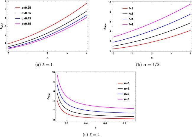
Figure 1. Energy levels Eℓ,m,n of equation ( |
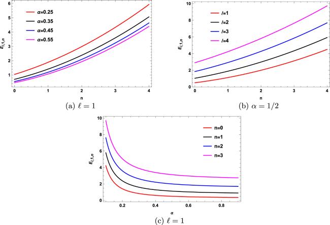
Figure 2. Energy levels Eℓ,m,n of equation ( |
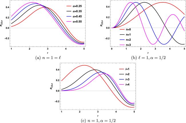
Figure 3. Radial wave function ${{ \mathcal R }}_{{\ell },m,n}$ of equation ( |
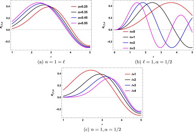
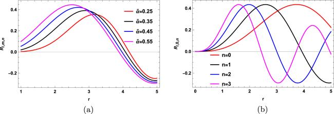
Figure 4. Radial wave function ${{ \mathcal R }}_{{\ell },m,n}$ of equation ( |
3. Global monopole effect on the solution of the Schrödinger equation with extended ring-shaped potential
3.1. Numerical examples of the eigenvalue solution
| 1. For m = 0 |
| • | If n = 0, we get: $\begin{eqnarray}{{\rm{\Psi }}}_{{\ell },\mathrm{0,0}}\left(r,\theta ,\varphi \right)={\tilde{C}}_{{\ell },\mathrm{0,0}}\ {r}^{-1/2}{J}_{{\tau }_{{\ell },0}}\left(\displaystyle \frac{\sqrt{2\,{E}_{{\ell },\mathrm{0,0}}}}{\tilde{\alpha }}\,r\right)\exp \left({\rm{i}}{\ell }\varphi \right),\end{eqnarray}$ and the associated energy level is, $\begin{eqnarray}{E}_{{\ell },\mathrm{0,0}}=\displaystyle \frac{1}{32}{\left(1\,+3\tilde{\alpha }\right)}^{2}\,\displaystyle \frac{{\pi }^{2}}{{r}_{0}^{2}},\end{eqnarray}$ with constraints, $\begin{eqnarray}{\lambda }_{{\ell },0}=0,\ {b}_{8}=0,\ {b}_{6}=-\displaystyle \frac{{{\ell }}^{2}}{4}.\end{eqnarray}$ |
| • | If n = 3, |
| 2. For m = 1 |
| • | If n = 1, we have: $\begin{eqnarray}\begin{array}{l}{{\rm{\Psi }}}_{{\ell },\mathrm{1,1}}\left(r,\theta ,\varphi \right)\\ \,={\tilde{C}}_{{\ell },\mathrm{1,1}}\ {r}^{-1/2}{J}_{{\tau }_{{\ell },1}}\left(\displaystyle \frac{\sqrt{2\,{E}_{{\ell },\mathrm{1,1}}}}{\tilde{\alpha }}\,r\right)\left(\sin \theta +\displaystyle \frac{\sqrt{2}}{2}\right)\,\exp \,\left({\rm{i}}{\ell }\varphi \right),\end{array}\end{eqnarray}$ the associated energy level is, $\begin{eqnarray}{E}_{{\ell },\mathrm{1,1}}=\displaystyle \frac{1}{32}{\left(3\,+7\tilde{\alpha }\right)}^{2}\,\displaystyle \frac{{\pi }^{2}}{{r}_{0}^{2}},\end{eqnarray}$ with constraints, $\begin{eqnarray}{\lambda }_{{\ell },1}=2,\ {b}_{8}=\displaystyle \frac{1}{\sqrt{2}},\ {b}_{6}=-\displaystyle \frac{{{\ell }}^{2}}{4}.\end{eqnarray}$ |
| • | If n = 2 , we get: $\begin{eqnarray}\begin{array}{l}{{\rm{\Psi }}}_{{\ell },\mathrm{1,2}}\left(r,\theta ,\varphi \right)\\ \,={\tilde{C}}_{{\ell },\mathrm{1,2}}\ {r}^{-1/2}{J}_{{\tau }_{{\ell },1}}\left(\displaystyle \frac{\sqrt{2\,{E}_{{\ell },\mathrm{1,2}}}}{\tilde{\alpha }}\,r\right)\left(\sin \theta -\displaystyle \frac{\sqrt{2}}{2}\right)\,\exp \,\left({\rm{i}}{\ell }\varphi \right),\end{array}\end{eqnarray}$ and the associated energy level is, $\begin{eqnarray}{E}_{{\ell },\mathrm{1,2}}=\displaystyle \frac{1}{32}{\left(3\,+11\tilde{\alpha }\right)}^{2}\,\displaystyle \frac{{\pi }^{2}}{{r}_{0}^{2}},\end{eqnarray}$ with constraints, $\begin{eqnarray}{\lambda }_{\ell ,1}=2,\ {b}_{8}=-\displaystyle \frac{1}{\sqrt{2}},\ {b}_{6}=-\displaystyle \frac{{\ell }^{2}}{4},\end{eqnarray}$ where ${\tau }_{{\ell },1}=\tfrac{3}{2\,\tilde{\alpha }}$ and ∣ℓ∣ = 0, 1, 2, …. |
| 3. For m = 2 |
| • | If n = 2 , we have: $\begin{eqnarray}\begin{array}{l}{{\rm{\Psi }}}_{{\ell },\mathrm{2,2}}\left(r,\theta ,\varphi \right)\\ \,={\tilde{C}}_{{\ell },\mathrm{2,2}}\ {r}^{-1/2}{J}_{{\tau }_{{\ell },2}}\left(\displaystyle \frac{\sqrt{2\,{E}_{{\ell },\mathrm{2,2}}}}{\tilde{\alpha }}\,r\right)\left({\sin }^{2}\theta -\displaystyle \frac{\sqrt{22}}{4}\sin \theta +\displaystyle \frac{1}{4}\right)\exp \left({\rm{i}}{\ell }\varphi \right),\end{array}\end{eqnarray}$ the associated energy level is, $\begin{eqnarray}{E}_{{\ell },\mathrm{2,2}}=\displaystyle \frac{1}{32}{\left(5\,+11\tilde{\alpha }\right)}^{2}\,\displaystyle \frac{{\pi }^{2}}{{r}_{0}^{2}},\end{eqnarray}$ with constraints, $\begin{eqnarray}{\lambda }_{{\ell },2}=6,\ {b}_{8}=-\displaystyle \frac{\sqrt{22}}{2},\ {b}_{6}=-\displaystyle \frac{{{\ell }}^{2}}{4}.\end{eqnarray}$ |
| • | If n = 3 , we obtain: $\begin{eqnarray}{{\rm{\Psi }}}_{{\ell },\mathrm{2,3}}\left(r,\theta ,\varphi \right)={\tilde{C}}_{{\ell },\mathrm{2,3}}\ {r}^{-1/2}{J}_{{\tau }_{{\ell },2}}\left(\displaystyle \frac{\sqrt{2\,{E}_{{\ell },\mathrm{2,3}}}}{\tilde{\alpha }}\,r\right)\left({\sin }^{2}\theta +\displaystyle \frac{\sqrt{22}}{4}\sin \theta +\displaystyle \frac{1}{4}\right)\exp \left({\rm{i}}{\ell }\varphi \right),\end{eqnarray}$ and the associated energy level is, $\begin{eqnarray}{E}_{{\ell },\mathrm{2,2}}=\displaystyle \frac{25}{32}{\left(1\,+3\tilde{\alpha }\right)}^{2}\,\displaystyle \frac{{\pi }^{2}}{{r}_{0}^{2}},\end{eqnarray}$ with constraints, $\begin{eqnarray}{\lambda }_{{\ell },2}=6,\ {b}_{8}=\frac{\sqrt{22}}{2},\ {b}_{6}=-\frac{{{\ell }}^{2}}{4},\end{eqnarray}$ where ${\tau }_{{\ell },2}=\tfrac{5}{2\,\tilde{\alpha }}$ and ∣ℓ∣ = 0, 1, 2,…. |
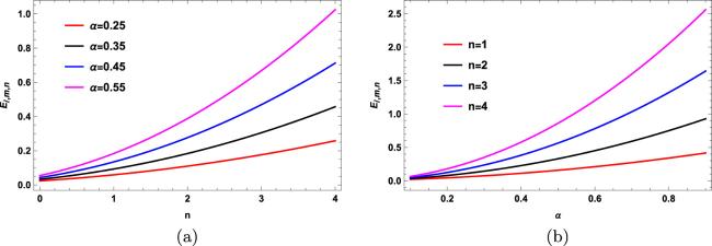
Figure 5. Energy levels Eℓ,m,n of equation ( |
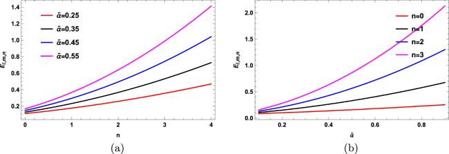
Figure 6. Energy levels Eℓ,m,n of equation ( |
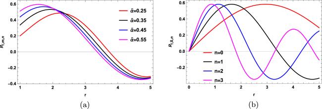
Figure 7. Radial wave function ${{ \mathcal R }}_{{\ell },m,n}$ of equation ( |
Figure 8. Radial wave function ${{ \mathcal R }}_{{\ell },m,n}$ of equation ( |