


1. Introduction
Dark matter (DM) remains one of the most enigmatic puzzles in the realm of particle physics and cosmology. Its existence, inferred from a multitude of astrophysical and cosmic scale observations, ranging from the rotation curves of galaxies and gravitational lensing to the precision measurements of the cosmic microwave background (CMB), highlights a significant void in our comprehension of the Universe's fundamental structure [1–4]. These observations provide compelling evidence of DM's gravitational influence; yet its precise particle physics properties continue to elude direct detection (DD). This presents not only a formidable challenge, but also an unprecedented opportunity for both theoretical and experimental physics to advance our understanding of particle physics.
Among the various candidates proposed to account for DM, the weakly interacting massive particles (WIMPs) stand out due to their compatibility with the relic density in the Universe [5–7]. WIMPs are theorized to have mass around the electroweak scale and engage in interactions at the weak interaction strength: characteristics that allow them to be thermally produced in the early universe via the freeze-out mechanism [8–10]. This process naturally results in a relic density that aligns with the CMB measurements, ΩDMh2 = 0.1192 ± 0.0010 [11], making WIMPs a compelling candidate for DM. However, the quest for DD of WIMPs through observations of nucleon recoil from DM–nucleon scattering has so far yielded no conclusive results. This challenge is largely attributed to the cross-symmetry that links the DD process with the freeze-out mechanism, underscoring the complexities associated with the direct detection of DM.
The investigation of top-quark philic DM has emerged as a compelling avenue to address the discrepancies between the null results from DD experiments and the observed DM relic density. The absence of the top quark in nucleons introduces a natural suppression mechanism for DD processes. Concurrently, the top quark's designation as the heaviest particle in the Standard Model (SM) and its essential role in electroweak symmetry breaking highlight its potential as a portal to DM [12, 13]. This paradigm has resulted in extensive research into the interaction dynamics of top-quark philic DM, aiming to evaluate its visibility through direct, indirect and collider search strategies. Such efforts represent a significant advancement in our quest to resolve DM, with DM models that interact with the top quark through high-dimensional operators posited for testing at the Large Hadron Collider (LHC) and in DM search experiments [14–17]. Models employing s-channel scalar mediators [18–20] or gauge boson mediators [21, 22] have been explored for collider implications. Additionally, numerous scalar DM models featuring a t-channel fermionic mediator have previously been examined [23–33].
The gauge boson mediator approach, particularly within the framework of $U{\left(1\right)}^{{\prime} }$ extended models [34], introduces the ${Z}^{{\prime} }$ gauge boson as the mediator [35–38]. The $U{\left(1\right)}^{{\prime} }$ gauge symmetry may arise from extensions of the SM gauge group [37], from unification models [39, 40] or from string theories [41, 42]. The gauge boson can acquire mass either through spontaneous symmetry breaking or via the Stueckelberg mechanism [43, 44]. For further details, see [34]. The top-quark philic model has been discussed in the context of DM [21], galactic gamma-ray lines [45, 46] and vacuum stability [47]. Simplified models of top-quark philic ${Z}^{{\prime} }$ have been studied in [48–50]. This ${Z}^{{\prime} }$ top-quark philic model has predominantly been investigated in the context of the LHC through top-quark pair association production [22, 48], single-top-quark associated production [51] or four top-quark productions [49–51]. With the associated production, the constraint on the ${Z}^{{\prime} }$ depends on both its coupling to the top quark and DM, namely the invisible decay branching ratio in the low-mass region. For instance, below the mass threshold for top-quark pair production, the coupling strength (gt) is typically constrained to about 0.5. However, for a very low mass around 100 GeV, the constraints are more dependent on the specific model [22]. Additionally, the ${Z}^{{\prime} }$'s impact on electroweak precision measurements has been studied [22, 52, 53], indicating that, without mixing between $U{\left(1\right)}^{{\prime} }$ and $U{\left(1\right)}_{Y}$, a lower bound of approximately 100 GeV is permitted for mV/gt. This limit varies, based on the details of the underlying theory and the degree of fine-tuning required.
In this work, we are dedicated to the DM narrative, with a focus on DD experiments. Adopting a general stance, we consider DM as a Dirac fermion interacting with the top quark via a gauge boson V. Our analysis of the DM relic density encompasses not only two-body processes, such as $\chi \bar{\chi }\to t\bar{t}$ and $\chi \bar{\chi }\to {VV}$, but also includes loop-generated processes $\chi \bar{\chi }\to {gg}$ and three-body processes $\chi \bar{\chi }\to t{\bar{t}}^{* }$, which become critical for low-mass DM particles χ. By examining the DM–nucleon scattering, we concentrate on the spin-independence interaction $(\bar{\chi }\chi {G}_{\mu \nu }^{a}\,{G}^{a\mu \nu })$, facilitated through two-loop corrections due to the top quark's absence in the nucleon.
The outline of this paper is as follows: in section 2 we set up the top-philic DM model, in which DM interacts with the SM via vector boson mediator particles. In section 3 , the model is constrained by the cosmological determination of the correct relic density of DM, and the effects arising from the presence of new resonance states are summarized. In section 4 , we calculate the σSI between DM and nucleons involving two-loop processes, obtaining the impact on DD constraints. We present our conclusion in section 5 .
2. Model setup
In this study, we adopt a simplified model framework to investigate the interactions between the DM and the SM particles, facilitated by a new mediator. We introduce a Dirac fermion, χ, as the DM candidate, and an additional vector boson, Vμ, serving as the mediator. This vector boson Vμ could represent an extended $U{\left(1\right)}^{{\prime} }$ gauge boson [34], engaging exclusively with the right-handed top quark [22]. The Lagrangian for our simplified model is expressed as follows:
$\begin{eqnarray}\begin{array}{l}{ \mathcal L }\supset {{ \mathcal L }}_{\mathrm{SM}}+\bar{\chi }\,({\rm{i}}{/}\!\!\!\!{\partial }-{m}_{\chi })\,\chi +\displaystyle \frac{1}{2}{V}^{\mu }\,(-\square -{m}_{V}^{2})\,{V}_{\mu }\\ \qquad +\bar{\chi }\,({a}_{\chi }+{b}_{\chi }\,{\gamma }_{5})\,{\gamma }^{\mu }\chi {V}_{\mu }+{g}_{t}\,\bar{t}{\gamma }^{\mu }{P}_{{\rm{R}}}\,{{tV}}_{\mu },\end{array}\end{eqnarray}$
where mV and mχ denote the masses of the vector boson Vμ and DM χ, respectively; PR is a right-handed projector operator, which ensures the gauge boson V couples with the right-handed top quark uniquely; aχ and bχ represent the vector and axial-vector current couplings between V and χ, respectively; gt represents the couplings between V and the top quark. To ensure the vector boson Vμ behaves as a narrow resonance, its total width must be less than about 10% of its mass mV. We initially examine the decay width of the vector boson Vμ. The principal decay modes at tree level are $V\to t\bar{t}$ and $V\to \chi \bar{\chi }$, provided the energy threshold is met. The three-body decay modes, such as $V\to t{\bar{t}}^{* }\,({t}^{* }\bar{t})$, and the loop-induced decay modes, V → W+W− and V → Zh, are considered negligible due to phase space and loop factor suppression. The partial decay widths of the tree-level processes $V\to t\bar{t}$ and $V\to \chi \bar{\chi }$ are given by: $\begin{eqnarray}\begin{array}{l}{\rm{\Gamma }}\,(V\to t\bar{t})=\displaystyle \frac{3{g}_{t}^{2}\,\sqrt{{m}_{V}^{2}-4{m}_{t}^{2}}}{48\pi {m}_{V}^{2}}\left[\left({m}_{V}^{2}+2{m}_{t}^{2}\right)\right.\\ \,\left.+\,\left({m}_{V}^{2}-4{m}_{t}^{2}\,\right) \right]{\rm{\Theta }}\left({m}_{V}-2{m}_{t}\right),\end{array}\end{eqnarray}$
$\begin{eqnarray}\begin{array}{l}{\rm{\Gamma }}\,(V\to \chi \bar{\chi })=\displaystyle \frac{\sqrt{{m}_{V}^{2}-4{m}_{\chi }^{2}}}{12\pi {m}_{V}^{2}}\left[{a}_{\chi }^{2}\left({m}_{V}^{2}+2{m}_{\chi }^{2}\right)\right.\\ \,\left.+\,{b}_{\chi }^{2}\left({m}_{V}^{2}-4{m}_{\chi }^{2}\,\right) \right]{\rm{\Theta }}\left({m}_{V}-2{m}_{\chi }\right),\end{array}\end{eqnarray}$
where mt represents the mass of the top quark, and Θ(x) denotes the Heaviside step function. The partial decay width of the V is displayed in figure 1. It is shown that the vector boson V is a narrow resonance for the parameter space of interest in the work. It is notable that the three-body decay process $V\to t{\bar{t}}^{* }$ is dominant over the loop-induced processes when the vector boson mass is larger than about 250 GeV.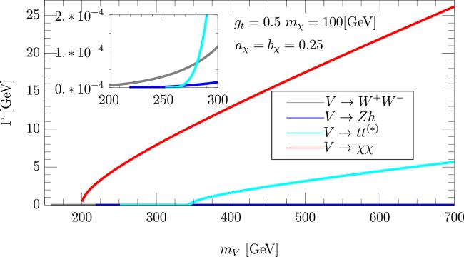
Figure 1. The partial decay width of the vector boson V as a function of the mass mV and DM mass fixed to mχ = 100 GeV. |
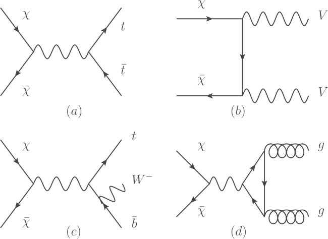
Figure 2. In this simplified model, DM annihilation involves tree-level two-body processes (a) and (b), a three-body process (c) and one-loop process (d), all contributing to DM relic abundance. |
3. Dark matter relic abundance
The Planck satellite experiment has conducted high-precision measurement of DM relic abundance, yielding the result ΩDMh2 = 0.1192 ± 0.0010. This measurement necessitates that the theoretical predictions for relic abundance in the simplified model should be lower than the observed value to prevent an excessive abundance of DM processes in the Universe. During the Universe's evolution, DM density can be calculated using the Boltzmann equation [7, 54]
$\begin{eqnarray}\begin{array}{l}\displaystyle \frac{{\rm{d}}{Y}}{{\rm{d}}{x}}=-\sqrt{\displaystyle \frac{\pi }{45}}{m}_{\mathrm{PL}}\,{m}_{\chi }\,\displaystyle \frac{{g}_{* s}\,{g}_{* }^{-1/2}}{{x}^{2}}\\ \quad \times \langle \sigma {v}_{\mathrm{rel}}\rangle \,[{Y}^{2}-{\left({Y}^{\mathrm{EQ}}\right)}^{2}],\end{array}\end{eqnarray}$
and its relic abundance is given by $\begin{eqnarray}{{\rm{\Omega }}}_{\chi }\,{h}^{2}\approx 2.76\times {10}^{8}Y\displaystyle \frac{{m}_{\chi }}{\mathrm{GeV}},\end{eqnarray}$
where Y is the DM number density of today in a comoving reference frame $\begin{eqnarray}Y=\sqrt{\displaystyle \frac{45}{\pi }}\displaystyle \frac{{g}_{\ast }{\left(\,{x}_{f}\,\right)}^{1/2}/{g}_{\ast s}\left(\,{x}_{f}\,\right)}{\left.{m}_{{\rm{PL}}}\,{m}_{\chi }\,\langle \sigma {v}_{{\rm{rel}}}\,\right\rangle }{x}_{f}.\end{eqnarray}$
Here, xf ≡ mχ/Tf, where Tf corresponds to the DM decoupling temperature and mPL = 1.22 × 10¹⁹ GeV corresponds to Planck mass. The g*(xf) and g*s(xf) correspond to the effective and entropic degrees of freedom at the DM decoupling temperature, respectively. Thus, the annihilation cross section ⟨σvrel⟩ corresponds to, $\begin{eqnarray}\langle \sigma {v}_{{\rm{rel}}}\rangle \approx 0.71\displaystyle \frac{0.12}{{{\rm{\Omega }}}_{\chi }\,{h}^{2}}\displaystyle \frac{{x}_{f}}{\,}\displaystyle \frac{{g}_{\ast }{\left(\,{x}_{f}\,\right)}^{1/2}/{g}_{\ast s}\left(\,{x}_{f}\,\right)}{0.1}\,{\rm{pb}}.\end{eqnarray}$
The annihilation cross section can be expanded in small amounts, depending on the velocity, i.e. $\langle \sigma {v}_{\mathrm{rel}}\rangle =a+b\,\langle {v}_{\mathrm{rel}}^{2}\rangle +{ \mathcal O }\,(\langle {v}_{\mathrm{rel}}^{4}\rangle )$. The coefficients a and b correspond to the contributions of s-wave and p-wave scattering, respectively.In the simplified model, DM pairs can annihilate into various final states, such as $\bar{t}t$, VV, gg and $t\bar{b}{W}^{-}$, depending on the properties of the involved particles [55–59]. For DM mass exceeding that of the top quark, χ can annihilate into a pair of top quarks via a resonance-mediated s-channel process. The thermally averaged cross section for this process is approximated as:
$\begin{eqnarray}\begin{array}{l}\langle \sigma {v}_{\mathrm{rel}}{\rangle }_{\chi \bar{\chi }\to t\bar{t}}\\ \simeq \displaystyle \frac{3{g}_{t}^{2}\,{\beta }_{t}\left[2{a}_{\chi }^{2}\,{\beta }_{t}^{2}\,{m}_{\chi }^{2}+{a}_{\chi }^{2}\left({m}_{t}^{2}+2{m}_{\chi }^{2}\right)+{\left({b}_{\chi }\,{\beta }_{\chi }^{2}\,{m}_{t}\,\right)}^{2}\right]}{8\pi {\left({\beta }_{\chi }\,{m}_{V}\,\right)}^{4}},\end{array}\end{eqnarray}$
where ${\beta }_{t}=\sqrt{1-{m}_{t}^{2}/{m}_{\chi }^{2}}$ and ${\beta }_{\chi }=\sqrt{1-4{m}_{\chi }^{2}/{m}_{V}^{2}}$ denote the velocities of the top quark and the DM, respectively. If mχ > mV, DM can also annihilate into a pair of vector bosons, with the thermally averaged cross section given by: $\begin{eqnarray}\begin{array}{l}\langle \sigma {v}_{\mathrm{rel}}{\rangle }_{\chi \bar{\chi }\to {VV}}\\ \quad \simeq \displaystyle \frac{{\beta }_{V}^{3}\left[({a}_{\chi }^{4}+{b}_{\chi }^{4})\,{m}_{V}^{2}+2{a}_{\chi }^{2}\,{b}_{\chi }^{2}\,(4{m}_{\chi }^{2}-3{m}_{V}^{2})\right]}{4\pi {m}_{\chi }^{2}\,{m}_{V}^{2}{\left(2-{m}_{V}^{2}/{m}_{\chi }^{2}\,\right)}^{2}},\end{array}\end{eqnarray}$
with ${\beta }_{V}=\sqrt{1-{m}_{V}^{2}/{m}_{\chi }^{2}}$ representing the velocity of the vector boson. Several points warrant emphasis regarding the above thermally averaged cross sections:| • | Equations ( |
| • | The $\chi \bar{\chi }\to t\bar{t}$ process, being s-channel, exhibits Breit–Wigner enhancement, especially when mχ ≃ mV/2. This effect is evident from the $1/{\beta }_{\chi }^{4}$ term in equation ( |
For scenarios where mχ < mt, three-body decay processes like $\bar{\chi }\chi \to t\bar{b}{W}^{-}$ and loop-induced processes such as $\bar{\chi }\chi \to {gg}$ become dominant in DM annihilation [60–62], surpassing $\chi \bar{\chi }\to t\bar{t}$. The thermally averaged cross section for $\bar{\chi }\chi \to {gg}$ is expressed as:
$\begin{eqnarray}\begin{array}{l}\langle \sigma {v}_{\mathrm{rel}}{\rangle }_{\chi \bar{\chi }\to {gg}}\simeq \displaystyle \frac{{\alpha }_{s}^{2}\,{g}_{t}^{2}\,{b}_{\chi }^{2}\,{m}_{\chi }^{2}\,({N}_{c}^{2}-1)}{64{\pi }^{2}{m}_{V}^{4}}\\ \quad \times {\left|\displaystyle \frac{\tau }{4}{\;\mathrm{ln}}^{2}\;\,\left[\displaystyle \frac{2\sqrt{1-\tau }+\tau -2}{\tau }\right]+1\right|}^{2}\;,\end{array}\end{eqnarray}$
where $\tau =4{m}_{t}^{2}/{q}^{2}$. It is clearly shown that the cross section only depends on the axial current interaction as it is generated from the axial anomaly. Notably, no Breit–Wigner enhancement is observed in this process, a consequence of the on-shell V process being forbidden by the Landau–Yang Theorem. It provides a detailed comparison between two DM annihilation processes in [15]. And it demonstrates that the loop-induced process $\chi \bar{\chi }\to {gg}$ predominates when the DM mass, mχ, is below approximately 130 GeV. Conversely, when mχ exceeds 130 GeV, the three-body process $\chi \bar{\chi }\to t\bar{b}{W}^{-}$ becomes the dominant mechanism influencing the DM relic abundance.In the following, we present our numerical results regarding the DM relic density. Using detailed computational analysis, we identify regions of parameter space that are consistent with the Planck satellite's measurement of the DM relic density, specifically focusing on the interplay between the coupling constants aχ, bχ and the DM mass mχ in figures 3 and 4. In figure 3, we delineate the parameter space (cyan shaded region) that aligns with the Planck satellite observations. This figure concentrates on the lower DM mass range, where two-body decay processes are kinematically forbidden. It is observed that, compared to loop-induced processes, the three-body process predominantly governs the parameter space. However, at a lower DM mass of approximately 150 GeV and a substantial coupling gt = 0.5, the loop contribution from the process $\chi \bar{\chi }\to {gg}$ becomes non-negligible. Figure 4 explores the DM relic density in the higher-mass regime, with the red line indicating the threshold Ωχh2 = 0.1198. Notably, a Breit–Wigner enhancement is evident around mχ ≃ mV/2, which allows for smaller couplings of gt to suffice; this effect is visibly represented as a valley in the red line. In the subplot of figure 4(b), we note a decrease in the couplings aχ and bχ as mχ exceeds mV, signifying the pivotal role of the $\chi \bar{\chi }\to {VV}$ process in the evolution of DM, especially when aχ = bχ ≈ 0.5. It is important to note the presence of a threshold effect in the right subplot when the DM mass exceeds the vector boson mass mV, an effect that is absent in the left subplot. This distinction arises because the annihilation mode $\chi \bar{\chi }\to {VV}$ predominates in the relic density calculation in the right plot, facilitated by the couplings gt = 0.2 in comparison to aχ = bχ ≈ 0.5. Conversely, in the left plot, the contribution from this mode is negligible relative to $\chi \bar{\chi }\to V\to t\bar{t}$, due to the stronger coupling gt = 0.5 and weaker aχ = bχ ≈ 0.2.
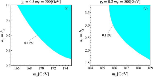
Figure 3. The relic density of DM χ plotted in the plane of coupling aχ (bχ) versus mass mχ, with the vector boson mass mV and its couplings to the top quark gt held constant. Subgraphs (a) and (b) show the numerical results for gt = 0.5 and gt = 0.2, respectively. The colored region indicates the parameter space that accommodates a relic density Ωχh2 ≤ 0.1192. Notably, the mass of the DM mχ is considered to be less than that of the top quark. |
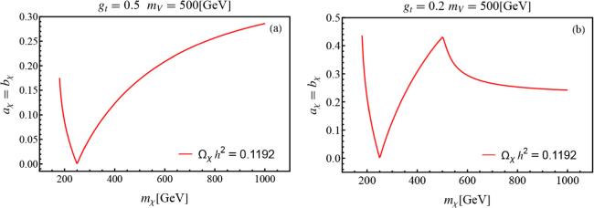
Figure 4. The relic density of DM χ, illustrated in the plane of coupling aχ (bχ) versus mass mχ, with the mass of the vector boson mV and its coupling to the top quark gt maintained constant. Subgraphs (a) and (b) show the numerical results for gt = 0.5 and gt = 0.2, respectively. The red line delineates Ωχh2 = 0.1192, and the DM mass mχ is considered to be larger than top-quark mass. |
Further analysis is presented in figure 5, which maps the DM relic density against the plane of mV and mχ for fixed couplings, focusing respectively on low and high DM mass regions. The cyan regions in these figures correspond to parameter spaces fulfilling the current measuring of DM relic abundance. Specifically, figures 5(a) and (b) employ two distinct sets of coupling constants: gt = 0.2 (0.5), and aχ = bχ = 0.1(0.25). In the domain of lower mχ, the significance of the three-body process is underscored, with resonance enhancement near 2mχ ∼ mV contributing to the achievement of the correct relic abundance. Conversely, figure 5 demonstrates that, in the regime of larger DM mass, two-body annihilation processes become dominant. With smaller couplings, as shown in figure 5(c), resonance enhancement is crucial for maintaining the DM relic density requirements, with the permissible parameter space concentrated around mχ ∼ mV/2. With larger couplings, as illustrated in figure 5(d), besides the enlarged parameter space around mχ ∼ mV/2, an additional parameter space for mχ > mV is also viable, due to the contribution from the $\chi \bar{\chi }\to {VV}$ process.

Figure 5. The relic density of DM χ displayed in the plane of vector boson mass mV and mχ with constant couplings gt, aχ, bχ. The colored region denotes the parameter space with Ωχh2 ≤ 0.1192. Subgraphs (a) and (b) correspond to smaller DM and intermediate mass, and subgraphs (c) and (d) correspond to larger DM mass and intermediate mass. In (c) and (d), the black line indicates the condition 2mχ ≈ mV, near which resonance enhancement is observed; the red dotted line marks the condition mχ ≈ mV. |
4. Dark matter direct detection
The DD experiments are one of the foundational approaches in the search for DM. The goal is to directly observe the rare scattering events between the non-relativistic DM particles and the target material. These scattering cross sections can be further categorized into spin-independent (SI) and spin-dependent (SD) contributions [63–68], reflecting the nature of the interaction between DM and the target nuclei. Since SI scattering interacts coherently with the entire nucleus, the cross section with respect to the target nucleon can be succinctly expressed as
$\begin{eqnarray}{\sigma }^{\mathrm{SI}}\,=\,\displaystyle \frac{4{\mu }_{\chi }^{2}}{\pi }{A}^{2}{\lambda }_{N}^{2},\end{eqnarray}$
which scales with the squared number of scattering centers (nucleons). Here, A is the atomic mass number of the target nuclei; μχ is the reduced mass of the DM–nucleon, defined as ${\mu }_{\chi }=\tfrac{{m}_{\chi }\,{m}_{N}}{({m}_{\chi }+{m}_{N})}$, and we treat mN as the mass of protons. The λN are the coupling constants of DM with the nucleon, defined as $\begin{eqnarray*}\begin{array}{l}{\lambda }_{p\,(n)}={m}_{N}\,\displaystyle \sum _{q=u,d,s}\,\,\left(\,{f}_{q}{f}_{{Tq}}+\displaystyle \frac{3}{4}\left(q\,(2)+\bar{q}\,(2),\,\right)\left({g}_{q}^{(1)}+{g}_{q}^{(2)} \right)\right)\\ \qquad -\displaystyle \frac{8\pi }{9{\alpha }_{s}}{f}_{{TG}}\,{f}_{G}+\displaystyle \frac{3}{4}G\,(2)\,\left({g}_{G}^{(1)}+{g}_{G}^{(2)}\right),\end{array}\end{eqnarray*}$
where fTq, fTG, q(2), $\bar{q}\,(2)$ and G(2) are hadronic matrix elements [69, 70] $\begin{eqnarray}\begin{array}{c}{m}_{f}\,{f}_{{Tq}}=\langle N|{m}_{q}\,\bar{q}q|N\rangle \,{f}_{{TG}}\equiv 1-\displaystyle \sum _{u,d,s}\,{f}_{{Tq}},\\ \langle N\,(\,p\,)\,|{{ \mathcal O }}_{\mu \nu }^{q}|N\,(\,p\,)\rangle =\displaystyle \frac{1}{{m}_{{\rm{N}}}}\,\left(\,{p}_{\mu }{p}_{\nu }-\displaystyle \frac{1}{4}{m}_{{\rm{N}}}^{2}\,{g}_{\mu \nu }\,(q\,(2)+\bar{q}\,(2)\right),\\ \langle N\,(\,p\,)\,|{{ \mathcal O }}_{\mu \nu }^{g}|N\,(\,p\,)\rangle =\displaystyle \frac{1}{{m}_{{\rm{N}}}}\,\left(\,{p}_{\mu }{p}_{\nu }-\displaystyle \frac{1}{4}{m}_{{\rm{N}}}^{2}\,{g}_{\mu \nu }\,G\,(2)\right),\end{array}\end{eqnarray}$
where mN is the nucleon mass and N is the proton or neutron. The values of hadronic matrix elements are given by [69] $\begin{eqnarray}\begin{array}{rcl}{f}_{{Tu}}^{p} & = & 0.018,\,\,{f}_{{Td}}^{p}=0.030,\,\,{f}_{{Tu}}^{n}=0.015,\\ {f}_{{Td}}^{n} & = & 0.034,\,\,{f}_{{TG}}=0.80,\end{array}\end{eqnarray}$
where fTqN corresponds to the contribution of the quark q to the nucleon matrix elements for the nucleon N. The matrix elements of the twist-2 operators are related to the second moments of the parton distribution functions (PDFs), $\begin{eqnarray}\begin{array}{l}q\,(2)+\bar{q}\,(2)={\displaystyle \int }_{0}^{1}\,{\rm{d}}{x}{x}\,(q\,(x)+\bar{q}\,(x)),\\ G\,(2)={\displaystyle \int }_{0}^{1}\,{\rm{d}}{x}{x}{g}\,(x),\end{array}\end{eqnarray}$
where $q\,(x),\,\bar{q}\,(x)$ and g(x) are the PDFs of the quark, anti-quark and gluon in nucleon N, respectively. Those hadronic elements could be extracted from the CT14NNLO PDFs [70], $\begin{eqnarray}\begin{array}{l}{\left[u\,(2)+\bar{u}\,(2)\right]}_{p}=0.3481,\,\,{\left[d\,(2)+\bar{d}\,(2)\right]}_{p}=0.1902,\\ G{\left(2\right)}_{p}=G{\left(2\right)}_{n}=0.4159.\end{array}\end{eqnarray}$
The fq, fG, ${g}_{q}^{(1)}$, ${g}_{q}^{(2)}$, ${g}_{G}^{(1)}$ and ${g}_{G}^{(2)}$ are Wilson coefficients of corresponding operators which describe the SI scattering. The effective Lagrangian [71, 72] exhibits as
$\begin{eqnarray}{ \mathcal L }\,=\,\displaystyle \sum _{u,d,s}\,{{ \mathcal L }}_{q}^{\mathrm{EFT}}+{{ \mathcal L }}_{g}^{\mathrm{EFT}},\end{eqnarray}$
where $\begin{eqnarray}\begin{array}{l}{{ \mathcal L }}_{q}^{\mathrm{EFT}}={f}_{q}\,{m}_{q}\,\bar{\chi }\chi \bar{q}q+\displaystyle \frac{{g}_{q}^{(1)}}{2{m}_{\chi }}\bar{\chi }i\,({\partial }^{\mu }{\gamma }^{\nu }+{\partial }^{\nu }{\gamma }^{\mu })\,\chi {O}_{q,\mu \nu }^{(2)}\\ \quad +\displaystyle \frac{{g}_{q}^{(2)}}{{m}_{\chi }^{2}}\bar{\chi }\,(i{\partial }^{\mu })\,(i{\partial }^{\nu })\,\chi {O}_{q,\mu \nu }^{(2)},\end{array}\end{eqnarray}$
$\begin{eqnarray}\begin{array}{l}{{ \mathcal L }}_{g}^{\mathrm{EFT}}={f}_{G}\,\bar{\chi }\chi {G}_{\,\mu \nu }^{a}\,{G}^{a\mu \nu }+\displaystyle \frac{{g}_{G}^{(1)}}{2{m}_{\chi }}\bar{\chi }i\,({\partial }^{\mu }{\gamma }^{\nu }+{\partial }^{\nu }{\gamma }^{\mu })\,\chi {O}_{G,\mu \nu }^{(2)}\\ \quad +\displaystyle \frac{{g}_{G}^{(2)}}{{m}_{\chi }^{2}}\bar{\chi }\,(i{\partial }^{\mu })\,(i{\partial }^{\nu })\,\chi {O}_{G,\mu \nu }^{(2)}.\end{array}\end{eqnarray}$
The twist-2 operators ${O}_{q,\mu \nu }^{(2)}$ and ${O}_{G,\mu \nu }^{(2)}$ are defined as
$\begin{eqnarray}{O}_{q,\mu \nu }^{(2)}\equiv \displaystyle \frac{1}{2}\bar{q}\,({\gamma }^{\{\mu \ }{{iD}}_{-}^{\ \nu \}}-\displaystyle \frac{{g}^{\mu \nu }}{4}i{/}\!\!\!\!{D}),\end{eqnarray}$
$\begin{eqnarray}{O}_{G,\mu \nu }^{\left(2\,\right)}\equiv -{G}^{a\mu \lambda }{G}_{\,\,\lambda }^{a\nu }+\displaystyle \frac{{g}^{\mu \nu }}{4}{\left(\,{G}_{\alpha \beta }^{a}\,\right)}^{2}.\end{eqnarray}$
Here, fq, fG, ${g}_{q}^{(1)}$, ${g}_{q}^{(2)}$, ${g}_{G}^{(1)}$ and ${g}_{G}^{(2)}$ could match to our simplified model.In the simplified model, the vector boson mediator uniquely interacts with the top quark in the SM; therefore, we focus on the DM–nucleon scattering induced from the operator $\bar{\chi }\chi {G}_{\,\mu \nu }^{a}\,{G}^{a\mu \nu }$ as the twist-2 operator denotes high-order effects. The operator is generated at the loop level in the simplified model. The one-loop contribution from the cross one of the DM annihilation process $\chi \bar{\chi }\to {gg}$ is highly suppressed and negligible. It is attributed from this that the mediator vector boson is on-shell for the non-relativistic DM scattering at the leading order and the process is forbidden by the Landau–Yang theorem. The leading-order contribution comes from the two-loop Feynman diagrams, see figure 6. The matching coefficients fG can be calculated using the usual method with the help of the projection operators. Alternatively, one can also use the Fock–Schwinger gauge to simplify the calculation [71, 73], i.e. xμAμ = 0. In this work, we will focus on the Fock–Schwinger gauge method and refer the reader to [74] for details of the projection operator approach. In the Fock–Schwinger gauge, one can express the gluon field in terms of its field strength tensor Gμν and maintain explicit gauge invariance for each step in the calculation. The Wilson coefficients can be extracted from the two-loop correction, and it showsappendix .
$\begin{eqnarray}\begin{array}{l}{f}_{G}=\displaystyle \int \displaystyle \frac{{{\rm{d}}}^{4}p}{{\left(2\pi \right)}^{4}}\left[({a}_{\chi }+{b}_{\chi }\,{\gamma }_{5})\,{\gamma }^{\alpha }\,[(\,{{/}\!\!\!\!{p}}_{\chi }-{/}\!\!\!\!{p\,})+{m}_{\chi }]\right.\\ \quad \left.\times ({a}_{\chi }+{b}_{\chi }\,{\gamma }_{5})\,{\gamma }^{\beta }\right]\\ \Space{0ex}{1.84em}{0ex}\quad \times \displaystyle \frac{\left[{g}_{\alpha \mu }-\tfrac{{p}_{\alpha }\,{p}_{\mu }}{{m}_{V}^{2}}\right]\,\left[{g}_{\beta \nu }-\tfrac{{p}_{\beta }\,{p}_{\nu }}{{m}_{V}^{2}}\right]}{(\,{p}^{2}-{m}_{V}^{2})\,(\,{p}^{2}-{m}_{V}^{2})\,[{\left(\,{p}_{\chi }-p\,\right)}^{2}-{m}_{\chi }^{2}]}{{ \mathcal M }}^{\mu \nu }\,(\,p\,),\end{array}\end{eqnarray}$
in the limit of zero momentum transfer, where pχ is the DM momentum and ${{ \mathcal M }}^{\mu \nu }\,(\,p\,)$ denotes the top-quark box diagram contribution in figure 7. Using the Fock–Schwinger gauge it is obtained $\begin{eqnarray}\begin{array}{l}{{ \mathcal M }}^{\mu \nu }={\displaystyle \int }_{0}^{1}{\rm{d}}{x}\left[\displaystyle \frac{{{ig}}_{s}^{2}{g}_{t}^{2}\left(4{x}^{2}{\left(x-1\right)}^{2}{p}^{\mu }{p}^{\nu }-{m}_{t}^{2}\left(\left(8{x}^{2}-8x+3\right)-\right){g}^{\mu \nu }\right)}{192{\pi }^{2}{{\rm{\Delta }}}^{2}}\right.\\ \quad +\displaystyle \frac{{{ig}}_{s}^{2}{g}_{t}^{2}{m}_{t}^{2}\left({m}_{t}^{2}\left(\left(2{x}^{2}-2x+1\right)+{\left(1-2x\right)}^{2}\right){g}^{\mu \nu }-4\left(3{x}^{3}-6{x}^{2}+4x-1\right){p}^{\mu }{p}^{\nu }\right)}{96{\pi }^{2}{{\rm{\Delta }}}^{3}}\left.\,+\,\displaystyle \frac{{{ig}}_{s}^{2}{g}_{t}^{2}x\left(1-x\right){g}^{\mu \nu }}{48{\pi }^{2}{\rm{\Delta }}}\right],\end{array}\end{eqnarray}$
where ${\rm{\Delta }}=x\,(x-1)\,{p}^{2}+{m}_{t}^{2}$. After integration, the Wilson coefficient of the gluon field can be expressed as $\begin{eqnarray}\begin{array}{rcl}{f}_{G} & = & {f}_{1}\,{A}_{0}\,({m}_{V}^{2})+{f}_{2}\,{A}_{0}\,({m}_{t}^{{\prime} 2})+{f}_{3}\,{B}_{0}\,(0,{m}_{t}^{{\prime} 2},{m}_{t}^{{\prime} 2})\\ & & +\,{f}_{4}\,{B}_{0}\,(0,{m}_{V}^{2},{m}_{V}^{2})+{f}_{5}\,{B}_{0}\,({m}_{\chi }^{2},{m}_{\chi }^{2},{m}_{t}^{{\prime} 2})\\ & & +\,{f}_{6}\,{B}_{0}\,({m}_{\chi }^{2},{m}_{V}^{2},{m}_{\chi }^{2})\\ & & +\,{f}_{7}\,{D}_{0}\,(0,0,{m}_{\chi }^{2},{m}_{\chi }^{2},0,{m}_{\chi }^{2},{m}_{t}^{{\prime} 2},{m}_{t}^{{\prime} 2},{m}_{t}^{{\prime} 2},{m}_{\chi }^{2})\\ & & +\,{f}_{8}\,{C}_{0}\,(0,{m}_{\chi }^{2},{m}_{\chi }^{2},{m}_{V}^{2},{m}_{V}^{2},{m}_{\chi }^{2})\\ & & +\,{f}_{9}\,{C}_{0}\,(0,{m}_{\chi }^{2},{m}_{\chi }^{2},{m}_{t}^{{\prime} 2},{m}_{t}^{{\prime} 2},{m}_{\chi }^{2})\\ & & +\,{f}_{10}\,{C}_{0}\,(0,0,0,{m}_{t}^{{\prime} 2},{m}_{t}^{{\prime} 2},{m}_{t}^{{\prime} 2}),\end{array}\end{eqnarray}$
where ${m}_{t}^{{\prime} }=\tfrac{{m}_{t}}{\sqrt{x\,(1-x)}}$, A0, B0, C0 and D0 are Passarino–Veltman scalar functions [75, 76]. The forms of f1 to f10 are given in the 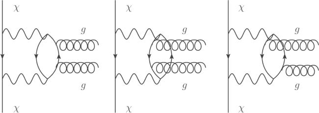
Figure 6. Two-loop Feynman diagrams depicting DM χ scattering with gluons. |
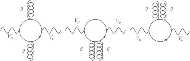
Figure 7. The box diagrams generating vector boson V scattering with gluons. |
Next, we perform the numeric results on the DM–nucleon SI cross section, namely
$\begin{eqnarray}{\sigma }_{\chi N}^{{\rm{SI}}}=\displaystyle \frac{256\pi {\mu }_{\chi }^{2}\,{m}_{{\rm{N}}}^{2}}{81{\alpha }_{s}^{2}}{f}_{{TG}}^{2}\,{f}_{G}^{2},\end{eqnarray}$
in comparison DM DD experiments. In figure 8, we illustrate the predicted cross sections for a simplified model with the parameters set at gt = 0.5 and aχ = bχ = 0.25. The contours of the SI scattering cross section $({\sigma }_{\chi N}^{\mathrm{SI}})$ are depicted with solid lines in blue, pink and gray. The current experimental PandaX-4T (0.63 t×y) [77] limits on ${\sigma }_{\chi N}^{\mathrm{SI}}$ for varying DM masses are shown by the solid black line, while future projections (XENOTnT(1000 t × y))[78] are represented by the dashed black line. Figure 8(a) presents the case where the DM mass (mχ) is less than the mass of the top quark. In this scenario, the SI scattering cross section between DM and nucleons typically ranges from 10−47 to 10−46 cm2. The current experimental limit on ${\sigma }_{\chi N}^{\mathrm{SI}}$ is about 10−46 cm2 for low-mass DM, indicating that this range remains largely unconstrained. However, future projections suggest that all of this parameter space could be explored in upcoming DM DD experiments. Figure 8(b) addresses the scenario where the DM mass exceeds the top-quark mass, enabling the annihilation process $\chi \bar{\chi }\to t\bar{t}$. Here, ${\sigma }_{\chi N}^{\mathrm{SI}}$ values range between 10−47 and 10−48 cm2, with portions already excluded by current DD experiments, as depicted by the solid black line. Particularly, the parameter space with vector boson masses below 200 GeV is inconsistent with current DD results. Future experiments are expected to probe the vector boson mass below 600 GeV, potentially testing much of the remaining parameter space.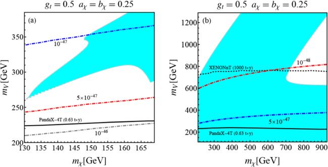
Figure 8. The DM–nucleon SI scattering cross section ${\sigma }_{\chi N}^{\mathrm{SI}}$ in the mV and mχ plane is illustrated. Subgraphs (a) and (b) correspond to numerical results for smaller/larger masses of DM and intermediate state, respectively. The colored dot–dashed lines indicate the contours of the cross sections. The solid and dashed black lines represent the results from the current DM DD experiment PandaX-4T (0.63 t×y) [77] and the projections for the future experiment XENONnT (1000 t×y) [78], respectively, with varying mχ. |
5. Conclusions
In this study, we concentrate on a specific category of simplified DM models characterized by exclusive interactions with the top quark. We introduce a Dirac-type DM particle, denoted as χ, and a vector-like intermediate particle, V, into the simplified model. The model incorporates a comprehensive interaction schema that includes both vector and axial-vector couplings to DM. We proceed to derive the DM relic density, accounting for contributions from three-body processes and loop-induced mechanisms, which are crucial for modeling low-mass DM scenarios. Subsequently, we calculate the SI DM–nucleon cross section, which arises from two-loop interactions, denoted as $\bar{\chi }\chi {GG}$.
In the low DM mass region, the resonance effect is necessary to achieve the DM relic abundance, even with large couplings (gt ≈ 0.5 and aχ ≈ bχ ≈ 0.25). In this regime, the three-body annihilation process $\chi \bar{\chi }\to t\bar{b}{W}^{-}$ predominates in the early Universe. Conversely, for DM with a larger mass, the two-body annihilation processes $\chi \bar{\chi }\to {VV}$ and $\chi \bar{\chi }\to t\bar{t}$ are dominant in determining the DM relic abundance. In DM DD experiments, the parameter space for low-mass DM will be probed in future experiments (XENOTnT (1000 t × y)) with moderate couplings (gt ≈ 0.5 and aχ ≈ bχ ≈ 0.25) [78]. For cases where mχ > 200 GeV, the parameter space has already been excluded by current experiments (PandaX-4T(0.63 t×y)) if the vector boson mass is below 200 GeV [77]. In future experiments, the parameter space will be testable if the vector boson mass is less than approximately 600 GeV.
Acknowledgments
We would like to thank Shuangshuang Hu for her valuable discussions. The work is supported in part by the National Science Foundation of China under Grant Nos. 12222502 and 12075257.
Appendix
A.1. Integral formula
$\begin{eqnarray}\displaystyle \frac{1}{{AB}}={\int }_{0}^{1}\,{\rm{d}}{x}\displaystyle \frac{1}{{\left[{xA}+(1-x)\,B\right]}^{2}},\end{eqnarray}$
$\begin{eqnarray}\displaystyle \frac{1}{{A}^{4}B}={\int }_{0}^{1}\,{\rm{d}}{x}\displaystyle \frac{4{x}^{3}}{{\left[{xA}+(1-x)\,B\right]}^{5}},\end{eqnarray}$
$\begin{eqnarray}\displaystyle \frac{1}{{{AB}}^{4}}\,=\,{\int }_{0}^{1}\,{\rm{d}}{x}\displaystyle \frac{4{\left(1-x\right)}^{3}}{{\left[{xA}+(1-x)\,B\right]}^{5}},\end{eqnarray}$
$\begin{eqnarray}\displaystyle \frac{1}{{A}^{2}{B}^{2}}\,=\,{\int }_{0}^{1}\,{\rm{d}}{x}\displaystyle \frac{6x\,(1-x)}{{\left[{xA}+(1-x)\,B\right]}^{4}}.\end{eqnarray}$
A.2. fn
The functions f1 ∼ f10, which are used in equation (4.13 ), are defined as
$\begin{eqnarray}\begin{array}{l}{f}_{1}=\displaystyle \frac{{g}_{s}^{2}\,({a}_{\chi }^{2}+{b}_{\chi }^{2})}{24{m}_{\chi }\,x\,(x-1)\,{\left({m}_{t}^{{\prime} 2}-{m}_{V}^{2}\,\right)}^{4}}\\ \quad \times \left[{a}_{\chi }^{2}\,(3{{m}_{t}^{{\prime} }}^{4}x\,(x-1)+{m}_{t}^{{\prime} 2}\,{m}_{V}^{2}\right.\\ \quad \times (10x-10{x}^{2}-3)+{m}_{V}^{4}\,x\,(x-1))\\ \quad -{b}_{\chi }^{2}\,({m}_{t}^{{\prime} 4}\,(-11{x}^{2}+11x-4)+{m}_{t}^{{\prime} 2}\,{m}_{V}^{2}\\ \quad \left.\times (-2{x}^{2}+2x+1)+{m}_{V}^{4}\,x\,(x-1))\right],\end{array}\end{eqnarray}$
$\begin{eqnarray}\begin{array}{l}{f}_{2}=\displaystyle \frac{{g}_{s}^{2}\,({a}_{\chi }^{2}+{b}_{\chi }^{2})}{24{m}_{\chi }\,x\,(x-1)\,{\left({m}_{t}^{{\prime} 2}-{m}_{V}^{2}\,\right)}^{4}}\\ \quad \times \left[{a}_{\chi }^{2}\,(-3{m}_{t}^{{\prime} 4}\,x\,(x-1)+{m}_{t}^{{\prime} 2}\,{m}_{V}^{2}\right.\\ \quad \times (10x-10{x}^{2}-3)-{m}_{V}^{4}\,x\,(x-1))\\ \quad +{b}_{\chi }^{2}\,({m}_{t}^{{\prime} 4}\,(11{x}^{2}-11x+4)+{m}_{t}^{{\prime} 2}\,{m}_{V}^{2}\\ \quad \left.\times (2{x}^{2}-2x-1)-{m}_{V}^{4}\,x\,(x-1))\right],\end{array}\end{eqnarray}$
$\begin{eqnarray}\begin{array}{l}{f}_{3}=\displaystyle \frac{{g}_{s}^{2}\,{g}_{t}^{2}}{192{m}_{\chi }\,x\,(x-1)\,{\left({m}_{t}^{{\prime} 2}-{m}_{V}^{2}\,\right)}^{3}}\\ \quad \times \left[({m}_{t}^{{\prime} 2}+{m}_{V}^{2}\,(8{x}^{2}-8x+3))\right.\\ \quad \left.+({m}_{t}^{{\prime} 2}\,(16{x}^{2}-16x+5)-{m}_{V}^{2})\right],\end{array}\end{eqnarray}$
$\begin{eqnarray}\begin{array}{l}{f}_{4}=\displaystyle \frac{{g}_{s}^{2}\,{g}_{t}^{2}}{192{m}_{\chi }\,x\,(x-1)\,{\left({m}_{t}^{{\prime} 2}-{m}_{V}^{2}\,\right)}^{3}}\\ \quad \times \left[({m}_{t}^{{\prime} 4}\,(6{x}^{2}-6x+1)-3{m}_{t}^{{\prime} 2}\,{m}_{V}^{2}{\left(1-2x\right)}^{2}\right.\\ \quad +2{m}_{V}^{2}\,x\,(x-1))\\ \quad \left.-(3{m}_{t}^{{\prime} 2}-{m}_{V}^{2})\,({m}_{t}^{{\prime} 2}\,(2{x}^{2}-2x+1)+2{m}_{V}^{2}\,x\,(x-1))\right],\end{array}\end{eqnarray}$
$\begin{eqnarray}\begin{array}{l}{f}_{5}=-{f}_{6}=\displaystyle \frac{{g}_{s}^{2}\,{g}_{t}^{2}}{192{m}_{\chi }\,x\,(x-1)\,{\left({m}_{t}^{{\prime} 2}-{m}_{V}^{2}\,\right)}^{4}}\\ \quad \times \left[\left({b}_{\chi }^{2}\,({m}_{t}^{{\prime} 6}\,(6{x}^{2}-6x+1)-4{m}_{t}^{{\prime} 2}\right.\right.\\ \quad \times ({m}_{V}^{2}\,(3{x}^{2}-3x+1)+2{m}_{\chi }^{2}\,(8{x}^{2}-8x+1))\\ \quad +{m}_{t}^{{\prime} 2}\,{m}_{V}^{2}\,({m}_{V}^{2}\,(-6{x}^{2}+6x-3)+4{m}_{\chi }\\ \quad \times (18{x}^{2}-18x+5))-8{m}_{V}^{4}\,{m}_{\chi }^{2}\,x\,(x-1))\\ \quad +{b}_{\chi }^{2}\,({m}_{t}^{{\prime} 6}\,(6{x}^{2}-6x+1)-4{m}_{t}^{{\prime} 4}\\ \quad \times ({m}_{V}^{2}\,(3{x}^{2}-3x+1)-3{m}_{\chi }^{2}\,x\,(x-1))\\ \quad -{m}_{t}^{{\prime} 2}\,{m}_{V}^{2}\,({m}_{V}^{2}\,(6{x}^{2}-6x+3)+4{m}_{\chi }^{2}\\ \quad \left.\times (10{x}^{2}-10x+3))+4{m}_{\chi }^{4}\,{m}_{\chi }^{2}\,x\,(x-1))\right)\\ \quad +\left({b}_{\chi }^{2}\,({m}_{t}^{{\prime} 6}\,(-6{x}^{2}+6x+3)-4{m}_{t}^{{\prime} 2}\right.\\ \quad \times ({m}_{V}^{2}\,(5{x}^{2}-5x+1)-2{m}_{\chi }^{2}\,(13{x}^{2}-13x+5))\\ \quad +{m}_{t}^{{\prime} 2}\,{m}_{V}^{2}\,({m}_{V}^{2}\,(2{x}^{2}+2x-1)-4{m}_{\chi }\,(6{x}^{2}-6x+7)\\ \quad -8{m}_{V}^{4}\,{m}_{\chi }^{2}\,x\,(x-1))\\ \quad +{a}_{\chi }^{2}\,({m}_{t}^{{\prime} 6}\,(-6{x}^{2}+6x-3)-4{m}_{t}^{{\prime} 4}\\ \quad \times ({m}_{V}^{2}\,(5{x}^{2}-5x+1)+{m}_{\chi }^{2}\,(11{x}^{2}-11x+4))\\ \quad +{m}_{t}^{{\prime} 2}\,{m}_{V}^{2}\,({m}_{V}^{2}\,(2{x}^{2}-2x+1)+4{m}_{\chi }^{2}\\ \quad \left.\left.\times (-2{x}^{2}+2x+1))+4{m}_{\chi }^{4}\,{m}_{\chi }^{2}\,x\,(x-1))\right)\right],\end{array}\end{eqnarray}$
$\begin{eqnarray}\begin{array}{l}{f}_{7}=\displaystyle \frac{{g}_{s}^{2}\,{g}_{t}^{2}\,{m}_{t}^{{\prime} 2}}{96{m}_{\chi }\,x\,(x-1)\,{\left({m}_{t}^{{\prime} 2}-{m}_{V}^{2}\,\right)}^{2}}\\ \quad \times \left[({a}_{\chi }^{2}\,({m}_{t}^{{\prime} 2}\,(2{x}^{2}-2x+1)-2{m}_{\chi }^{2})\right.\\ \quad +{a}_{\chi }^{2}\,(2{x}^{2}-2x+1)\,({m}_{t}^{{\prime} 2}+2{m}_{\chi }^{2}))\\ \quad +({b}_{\chi }^{2}\,({m}_{t}^{{\prime} 2}{\left(1-2x\right)}^{2}-2{m}_{\chi }^{2}\,(6{x}^{2}-6x+1))\\ \quad \left.+{a}_{\chi }^{2}\,(1-2x)\,({m}_{t}^{{\prime} 2}+2{m}_{\chi }^{2}))\right],\end{array}\end{eqnarray}$
$\begin{eqnarray}\begin{array}{l}{f}_{8}=-\displaystyle \frac{{g}_{s}^{2}\,{g}_{t}^{2}}{192{m}_{\chi }\,x\,(x-1)\,{\left({m}_{t}^{{\prime} 2}-{m}_{V}^{2}\,\right)}^{3}}\\ \quad \times \left[[{b}_{\chi }^{2}\,({m}_{t}^{{\prime} 4}\,(6{x}^{2}-6x+1)\,({m}_{V}^{2}-6{m}_{\chi }^{2})\right.\\ \quad +{m}_{t}^{{\prime} 2}\,(2{m}_{V}^{2}\,{m}_{\chi }^{2}\,(22{x}^{2}-22x+5)\\ \quad -3{m}_{V}^{4}{\left(1-x\right)}^{2})+2{m}_{V}^{4}\,x\,(x-1)\,({m}_{V}^{2}-4{m}_{\chi }^{2}))\\ \quad +{a}_{\chi }^{2}\,({m}_{V}^{2}+2{m}_{\chi }^{2})\,({m}_{t}^{{\prime} 4}\,(6{x}^{2}-6x+1)\\ \quad -3{m}_{t}^{{\prime} 2}\,{m}_{V}^{2}{\left(1-2x\right)}^{2}+2{m}_{V}^{4}\,x\,(x-1))]\\ \quad +[{a}_{\chi }^{2}\,(-2{m}_{t}^{{\prime} 4}\,(2{x}^{2}-2x+1)\,({m}_{V}^{2}-6{m}_{\chi }^{2})\\ \quad +{m}_{t}^{{\prime} 2}\,({m}_{V}^{4}\,(-4{x}^{2}+4x+1)-2{m}_{V}^{2}\,{m}_{\chi }^{2}\,(2{x}^{2}-2x+7))\\ \quad +2{m}_{V}^{2}\,x\,(x-1)\,({m}_{V}^{2}-4{m}_{\chi }^{2}))\\ \quad +{a}_{t}^{2}\,(3{m}_{t}^{{\prime} 4}-{m}_{V}^{2})\,({m}_{V}^{2}+2{m}_{\chi }^{2})\\ \quad \left.\times ({m}_{t}^{{\prime} 2}\,(2{x}^{2}-2x+1)+2{m}_{V}^{2}\,x\,(x-1))]\right],\end{array}\end{eqnarray}$
$\begin{eqnarray}\begin{array}{l}{f}_{9}=-\displaystyle \frac{{g}_{s}^{2}\,{g}_{t}^{2}\,{m}_{t}^{{\prime} 2}}{192{m}_{\chi }\,x\,(x-1)\,{\left({m}_{t}^{{\prime} 2}-{m}_{V}^{2}\,\right)}^{3}}\\ \quad \times \left[[{b}_{\chi }^{2}\,({m}_{t}^{{\prime} 4}{\left(1-2x\right)}^{2}-{m}_{t}^{{\prime} 2}\right.\\ \quad \times ({m}_{V}^{2}\,(12{x}^{2}-12x+5)+2{m}_{\chi }^{2}\,(14{x}^{2}-14x+1))\\ \quad +2{m}_{V}^{2}\,{m}_{\chi }^{2}\,(14{x}^{2}-14x+5))+{b}_{\chi }^{2}\,({m}_{t}^{{\prime} 4}{\left(1-2x\right)}^{2}-{m}_{t}^{{\prime} 2}\\ \quad \times ({m}_{V}^{2}\,(12{x}^{2}-12x+5)+2{m}_{\chi }^{2})\\ \quad -2{m}_{V}^{2}\,{m}_{\chi }^{2}\,(8{x}^{2}-8x+3))]+[{b}_{\chi }^{2}\,({m}_{t}^{{\prime} 4}\\ \quad \times (8{x}^{2}-{x}^{2}+3)+{m}_{t}^{{\prime} 2}\,({m}_{V}^{2}\,(8{x}^{2}-8x+1)\\ \quad -2{m}_{\chi }^{2}\,(34{x}^{2}-34x+1))+2{m}_{V}^{2}\,{m}_{\chi }^{2}\,(10{x}^{2}-10x+7))\\ \quad +{b}_{t}^{2}\,({m}_{t}^{{\prime} 4}\,(8{x}^{2}-8x+3)\\ \quad +{m}_{t}^{{\prime} 2}\,({m}_{V}^{2}\,(8{x}^{2}-8x+1)+2{m}_{\chi }^{2}\,(16{x}^{2}-16x+5))\\ \quad \left.-2{m}_{V}^{2}\,{m}_{\chi }^{2})]\right],\end{array}\end{eqnarray}$
$\begin{eqnarray}\begin{array}{l}{f}_{10}=\displaystyle \frac{{g}_{s}^{2}\,{g}_{t}^{2}\,{m}_{t}^{{\prime} 4}\,({a}_{\chi }^{2}+{b}_{\chi }^{2})}{192{m}_{\chi }\,x\,(x-1)\,{\left({m}_{t}^{{\prime} 2}-{m}_{V}^{2}\,\right)}^{2}}\\ \qquad \times (6{x}^{2}-6x+2).\end{array}\end{eqnarray}$