


1. Introduction
The theory of optical solitons, which has been a vital part of the modern scientific community and has been crucial to several scientific disciplines, including engineering [1], plasma physics [2], telecommunications [3] and nonlinear dynamics has been a relatively active field of study in the last few decades [4]. The nonlinear Schrödinger equation (NLSE) is one of the most prominent dynamical models used to study pulse propagation in Kerr media [5]. A chirp frequency is produced by self-phase modulation and anomalous dispersion working together to balance out the Kerr effect [6]. When dispersion and nonlinear effects are accurately synchronised, chip-free pulses are generated [7]. Solitons are self-trapped wave packets with special properties [8]. They spread quickly and maintain their original character in the face of outside disturbances [9]. Along with other waves, researchers have been studying optical solitons for a number of decades [10]. The nonlinear dynamical structure can be used to explain complicated waveforms in fiber-optic telecommunications in a variety of manners [11] also it constitutes one of the methods used to understand and forecast quantum phenomena [12]. In literature the NLSE has remarkable applications in different fields, such as soliton theory [13], modern physics [14], ionized mechanics [15], sea water [16], optics [17], quantum mechanics [18] and also in other fields of physical sciences [19].
In the literature, eminent researchers adopted many unique types of methodologies for dealing with many complex models including the NLSE that can also be analysed with various analytical strategies such as the Hirota bilinear method [20], the Jacobi elliptic expansion method [21], the modified Khater method [22], the function expansion method [23], the variational iteration method [24], the Darboux transformation method [25], the linear superposition technique [26] the Riccati equation method [27], the exp(-φ(ψ)) expansion method [28], the inverse scaling transformation [29], the F expansion technique [30] and the homogeneous balance method [31].
The (1+1)-dimensional nonlinear chiral Schrödinger equation [32], is defined as
$\begin{eqnarray}\begin{array}{l}i{{ \mathcal W }}_{t}+{{ \mathcal W }}_{{xx}}-i\beta \left({{ \mathcal W }}^{* }{{ \mathcal W }}_{x}-{ \mathcal W }{{ \mathcal W }}_{x}^{* }\right){ \mathcal W }+\tau { \mathcal W }{\gamma }_{t}=0,\\ i=\sqrt{-1},\end{array}\end{eqnarray}$
where ${ \mathcal W }(x,t)$ denotes the complex function of variables x and t, while ${ \mathcal W }{\left(x,t\right)}^{* }$ is the conjugate of the complex function, β represents the constant of nonlinear interaction. The time-varying derivative of the ordinary Wiener procedure γ(t) is termed as ${\gamma }_{t}\,=\,\tfrac{d\gamma }{{\rm{d}}{t}}$. The Brownian motion is another name for the ordinary Wiener procedure, which is an unpredictable phenomenon that serves as the foundation for the study of probabilistic inequality equations. The expression Brownian was developed by Robert Brown in 1827, who initially published actual findings about the inconsistent behaviour of particles of pollen stabbed by particles of water [33].If we insert τ = 0, in equation (1 ), then the resulting model is an important type of nonlinear evolution equation that has applications in the fields of optics, ionised science, particle physics, and in other applied disciplines of mathematical sciences. In the literature, equation (1 ) is studied by Nishino et al to obtain the wave solution [34], and Bulutet al investigated the given model by using the sine-Gordon expansion method [35]. Currently, we aim to apply the modified extended tanh function method [36], the improved F-expansion method [37], and the unified method [38], to explore the governing model analytically. The developed solutions are newly made and unique because these techniques are not applied in previous literature to this model. Additionally, it is declared that the analyses performed during this work is highly valuable and of great importance in various fields of mathematical sciences, physics and many other optical transmission-of-data areas.
The paper is laid out as follows; in the current section we discuss the model background and introduction, whereas in section 2 , the description of the applied strategy is discussed in detail. The soliton solution of the suggested model are attained in section 3 , and the plot representation of the obtained solutions are included in section 4 , while the stability analysis of the solutions are in section 5 . And the conclusion of the article is summarized in section 6 .
2. Methodology
We assume the general form of PDE as,3 ) in (2 ), which gives the ODE as,
$\begin{eqnarray}F({ \mathcal W },{{ \mathcal W }}_{x},{{ \mathcal W }}_{t},{{ \mathcal W }}_{{xx}},{{ \mathcal W }}_{{tt}},{{ \mathcal W }}_{{xt}},\cdots )=0,\end{eqnarray}$
where F denotes the polynomial, and ${ \mathcal W }(x,t)$ is a complex function of variable x and t. $\begin{eqnarray}\begin{array}{l}{ \mathcal W }(x,t)={e}^{{\rm{i}}\zeta }{ \mathcal U }(\phi ),\\ \phi =q(x-2\rho t),\,\zeta =\tau \gamma (t)+\sigma t+\rho x,\end{array}\end{eqnarray}$
then we insert equation ( $\begin{eqnarray}G({ \mathcal U },{ \mathcal U }^{\prime} ,{ \mathcal U }^{\prime\prime} ,{ \mathcal U }\prime\prime\prime ,\cdots )=0.\end{eqnarray}$
2.1. The modified extended tan hyperbolic function method
The main steps of this method are discussed here in detail:
Step 1: The solution to equation (4 ) can be assumed as
$\begin{eqnarray}{ \mathcal U }(\phi )={s}_{0}+\displaystyle \sum _{i=1}^{n}{s}_{i}{\psi }^{i}(\phi )+\displaystyle \sum _{i=1}^{n}\displaystyle \frac{{m}_{i}}{{\psi }^{i}(\phi )}.\end{eqnarray}$
The variables s0, si, and mi denote the constant and ψ(φ) satisfies the condition $\begin{eqnarray}\psi ^{\prime} (\phi )=f+\psi {\left(\phi \right)}^{2},\end{eqnarray}$
where, f is a constant, then the solution is written asCase I. If f < 0, then the required solution has the form,4 ).
$\begin{eqnarray*}\begin{array}{rcl}\psi (\phi ) & = & -\sqrt{-f}\tanh \left(\sqrt{-f}\phi \right),\\ \psi (\phi ) & = & -\sqrt{-f}\coth \left(\sqrt{-f}\phi \right).\end{array}\end{eqnarray*}$
Case II. If f = 0, then the required solution has the form, $\begin{eqnarray*}\psi (\phi )=-\displaystyle \frac{1}{\phi }.\end{eqnarray*}$
Case III. If f > 0, then the required solution has the form, $\begin{eqnarray*}\begin{array}{rcl}\psi (\phi ) & = & \sqrt{f}\tan \left(\sqrt{f}\phi \right),\\ \psi (\phi ) & = & -\sqrt{f}\cot \left(\sqrt{f}\phi \right).\end{array}\end{eqnarray*}$
Step 2: In this step we firstly find the balancing number n, through utilizing the balancing approaches in equation (Step 3: Then we insert equation (5 ) and equation (6 ) in equation (4 ), and after this we collect the same power of ψi(φ)( −N≤ i ≤ N) equal to zero and get a system of mathematical equations. On solving these systems, one can get the required solutions.
2.2. The improved F-expansion technique
The main steps of this method are discussed here in detail as of follows,
Step 1: The solution to equation (4 ) can be assumed as,
$\begin{eqnarray}{ \mathcal U }(\phi )=\displaystyle \sum _{i=-n}^{n}{s}_{i}{\left(a+A(\phi )\right)}^{i},\end{eqnarray}$
where ni and a denote the constant and A(φ) satisfies the condition $\begin{eqnarray}A^{\prime} (\phi )=A{\left(\phi \right)}^{2}+\delta ,\end{eqnarray}$
where δ is a constant. Then the solution of a given system is as the following.Case I: If δ < 0, then hyperbolic function type solution has the form:
$\begin{eqnarray*}\begin{array}{rcl}A(\phi ) & = & -\sqrt{-\delta }\tanh \left(\sqrt{-\delta }\phi \right),\\ A(\phi ) & = & -\sqrt{-\delta }\coth \left(\sqrt{-\delta }\phi \right).\end{array}\end{eqnarray*}$
Case II: If δ > 0, then trigonometric function type solution has the form:
$\begin{eqnarray*}\begin{array}{rcl}A(\phi ) & = & \sqrt{\delta }\tan \left(\sqrt{\delta }\phi \right),\\ A(\phi ) & = & -\sqrt{\delta }\cot \left(\sqrt{\delta }\phi \right).\end{array}\end{eqnarray*}$
Case III: If δ = 0, then rational function-type solution has the form:
$\begin{eqnarray*}A(\phi )=-\displaystyle \frac{1}{\phi }.\end{eqnarray*}$
Step 2: In this step we firstly find the balancing number n, through utilizing the balancing approaches in equation (4 ).
Step 3: Then we insert equation (7 ) and equation (8 ) in equation (4 ), after this we collect the same power of A(φ) equal to zero and get a system of mathematical equations. On solving these systems, one can get the required solutions.
2.3. The unified method
The main steps of this method are discussed here in detail as the following.
Step 1: The solution to equation (4 ) can be assumed to be,
$\begin{eqnarray}{ \mathcal U }(\phi )={s}_{0}+\displaystyle \sum _{i=1}^{N}\left({d}_{i}{\psi }^{-i}(\phi )+{s}_{i}{\psi }^{i}(\phi )\right),\end{eqnarray}$
where, ψ(φ) satisfies the condition $\begin{eqnarray}\psi ^{\prime} (\phi )=\vartheta +\psi {\left(\phi \right)}^{2},\end{eqnarray}$
and $\psi ^{\prime} (\phi )=\tfrac{d\psi }{d\phi }$ , si, di and ϑ represent the constant. Then we write the solutions of a given system as,Family 1: If ϑ < 0, then the hyperbolic function-type solution has the form
$\begin{eqnarray}\psi (\phi )=\left\{\begin{array}{l}\displaystyle \frac{\sqrt{\vartheta \left(-\left({S}^{2}+{W}^{2}\right)\right)}-\sqrt{-\vartheta }\cosh \left(2\sqrt{-\vartheta }(P+\phi )\right)}{S\sinh \left(2\sqrt{-\vartheta }(P+\phi )\right)+W},\\ \displaystyle \frac{-S\sqrt{-\vartheta }\cosh \left(2\sqrt{-\vartheta }(P+\phi )\right)-\sqrt{\vartheta \left(-\left({S}^{2}+{W}^{2}\right)\right)}}{S\sinh \left(2\sqrt{-\vartheta }(P+\phi )\right)+W},\\ +\sqrt{-\vartheta }-\displaystyle \frac{2S\sqrt{-\vartheta }}{-\sinh \left(2\sqrt{-\vartheta }(P+\phi )\right)+\cosh \left(2\sqrt{-\vartheta }(P+\phi )\right)+S},\\ \displaystyle \frac{+2S\sqrt{-\vartheta }}{\sinh \left(2\sqrt{-\vartheta }(P+\phi )\right)+\cosh \left(2\sqrt{-\vartheta }(P+\phi )\right)+S}-\sqrt{-\vartheta },\end{array}\right.\end{eqnarray}$
where, S, W and ϑ denote the constant terms.Family 2: If ϑ > 0, then the parabolic function-type solution has the form
$\begin{eqnarray}\psi (\phi )=\left\{\begin{array}{l}\displaystyle \frac{+\sqrt{\vartheta \left({S}^{2}-{W}^{2}\right)}-S\sqrt{\vartheta }\cos \left(2\sqrt{\vartheta }(P+\phi )\right)}{S\sin \left(2\sqrt{\vartheta }(P+\phi )\right)+W},\\ \displaystyle \frac{-S\sqrt{\vartheta }\cos \left(2\sqrt{\vartheta }(P+\phi )\right)-\sqrt{\vartheta \left({S}^{2}-{W}^{2}\right)}}{S\sin \left(2\sqrt{\vartheta }(P+\phi )\right)+W},\\ +i\sqrt{\vartheta }-\displaystyle \frac{2{\rm{i}}{S}\sqrt{\vartheta }}{-i\sin \left(2\sqrt{\vartheta }(P+\phi )\right)+\cos \left(2\sqrt{\vartheta }(P+\phi )\right)+S},\\ \displaystyle \frac{+2i{S}\sqrt{\vartheta }}{i\sin \left(2\sqrt{\vartheta }(P+\phi )\right)+\cos \left(2\sqrt{\vartheta }(P+\phi )\right)+S}-i\sqrt{\vartheta },\end{array}\right.\end{eqnarray}$
where, S, W and ϑ denote the constant terms.Family 3: If ϑ = 0, then the rational function-type solution has the form
$\begin{eqnarray}\psi (\phi )=-\displaystyle \frac{1}{P+\phi }.\end{eqnarray}$
Step 2: In this step we firstly find the balancing number n, through utilizing the balancing approaches in equation (4 ).
Step 3: Then we insert equations (9 ) and (10 ) in (4 ), and after this we collect the same power of ψ(φ) equal to zero and get a system of mathematical equations. On solving these systems, one can get the required solutions.
3. Traveling wave solutions
Consider the transformation of the form [32], 14 ) and equation (15 ) into equation (1 ), which gives the ODE as
$\begin{eqnarray}\begin{array}{rcl}{ \mathcal W }(x,t) & = & {e}^{i\zeta }{ \mathcal U }(\phi ),\,\phi =q(x-2\rho {\rm{t}}),\\ \zeta & = & \tau \gamma (t)+\sigma t+\rho x,\end{array}\end{eqnarray}$
where the q, σ, ρ denote the constants and τ represents the strength of the noise. Further we write, $\begin{eqnarray}\left\{\begin{array}{l}\displaystyle \frac{d{ \mathcal W }}{d{t}}=(-2q\rho { \mathcal U }^{\prime} +i\sigma { \mathcal U }+i\tau { \mathcal U }{\gamma }_{t}){e}^{{\rm{i}}\zeta }\\ \displaystyle \frac{d{ \mathcal W }}{d{x}}=(q{ \mathcal U }^{\prime} +i\rho { \mathcal U }){e}^{{\rm{i}}\zeta }\\ \displaystyle \frac{d{ \mathcal W }* }{d{x}}=(q{ \mathcal U }^{\prime} -i\rho { \mathcal U }){e}^{{\rm{i}}\zeta }\\ \displaystyle \frac{{d}^{2}{ \mathcal W }}{{d{x}}^{2}}=({q}^{2}{ \mathcal U }^{\prime\prime} +2i{q}\rho { \mathcal U }^{\prime} -{\rho }^{2}{ \mathcal U }){e}^{{\rm{i}}\zeta }.\end{array}\right.\end{eqnarray}$
Insert equation ( $\begin{eqnarray}-\left(\sigma +{\rho }^{2}\right){ \mathcal U }+{q}^{2}{ \mathcal U }^{\prime\prime} +2\beta \rho {{ \mathcal U }}^{3}=0.\end{eqnarray}$
3.1. Application of the modified extended $\tanh $ function method
To obtain the soliton solution of equation (1 ), we first calculate n = 1 by using the approach of homogeneous balance in equation (16 ) and the equation (16 ) solution, which can be written in this way:17 ) along with (6 ) into (16 ), this gives the system of equations as a result.
$\begin{eqnarray}{ \mathcal U }(\psi )={s}_{0}+{s}_{1}\psi (\phi )+\displaystyle \frac{{m}_{1}}{\psi (\phi )}.\end{eqnarray}$
Further, by inserting ( $\begin{eqnarray*}\begin{array}{l}2{q}^{2}{s}_{1}+2\beta \rho {s}_{1}^{3}=0,\\ 12\beta \rho {m}_{1}{s}_{1}{s}_{0}+2\beta \rho {s}_{0}^{3}-\rho {s}_{0}-\sigma {s}_{0}=0,\\ 2{f}^{2}{m}_{1}{q}^{2}+2\beta \rho {m}_{1}^{3}=0,6\beta \rho {m}_{1}^{2}{s}_{0}=0,\\ 2{{fm}}_{1}{q}^{2}-{m}_{1}\rho +6\beta \rho {m}_{1}{s}_{0}^{2}+6\beta \rho {m}_{1}^{2}{s}_{1}-{m}_{1}\sigma =0,\\ 2{{fq}}^{2}{s}_{1}+6\beta \rho {m}_{1}{s}_{1}^{2}+6\beta \rho {s}_{0}^{2}{s}_{1}-\rho {s}_{1}-\sigma {s}_{1}=0.\end{array}\end{eqnarray*}$
Solve the given system of equations to reach the following outcomes:Family 1:
$\begin{eqnarray*}{s}_{0}=0,\,{s}_{1}=\displaystyle \frac{i{q}}{\sqrt{\beta \rho }},\,{m}_{1}=\displaystyle \frac{i{fq}}{\sqrt{\beta \rho }}.\end{eqnarray*}$
Case 1. If f < 0, then the solution is attained as $\begin{eqnarray}\begin{array}{l}{{ \mathcal W }}_{1}(x,t)=\left(-\displaystyle \frac{\coth \left(\sqrt{-f}q(x-2\rho {\rm{t}})\right)\left(\gamma t\tau +\sigma t+\rho {x}_{1}\right)}{\sqrt{-f}}\right.\\ \left.\quad -\displaystyle \frac{i\sqrt{-f}q\tanh \left(\sqrt{-f}q(x-2\rho {\rm{t}})\right)}{\sqrt{\beta \rho }}\right)\times {e}^{i\zeta },\end{array}\end{eqnarray}$
$\begin{eqnarray}\begin{array}{l}{{ \mathcal W }}_{2}(x,t)=\left(-\displaystyle \frac{\tanh \left(\sqrt{-f}q(x-2\rho {\rm{t}})\right)\left(\gamma t\tau +\sigma t+\rho {x}_{1}\right)}{\sqrt{-f}}\right.\\ \left.\quad -\displaystyle \frac{i\sqrt{-f}q\coth \left(\sqrt{-f}q(x-2\rho {\rm{t}})\right)}{\sqrt{\beta \rho }}\right)\times {e}^{i\zeta }.\end{array}\end{eqnarray}$
Case 2. If f = 0, then the solution is attained as $\begin{eqnarray}\begin{array}{l}{{ \mathcal W }}_{3}(x,t)=\left(-\displaystyle \frac{{i{fq}}^{2}(x-2\rho {\rm{t}})}{\sqrt{\beta \rho }}\right.\\ \quad \left.-\displaystyle \frac{i}{\sqrt{\beta \rho }(x-2\rho {\rm{t}})}\right)\times {e}^{i\zeta }.\end{array}\end{eqnarray}$
Case 3. If f > 0, then the solution is attained as $\begin{eqnarray}\begin{array}{l}{{ \mathcal W }}_{4}(x,t)=\left(\displaystyle \frac{i\sqrt{f}q\tan \left(\sqrt{f}q(x-2\rho {\rm{t}})\right)}{\sqrt{\beta \rho }}\right.\\ \quad \left.+\displaystyle \frac{i\sqrt{f}q\cot \left(\sqrt{f}q(x-2\rho {\rm{t}})\right)}{\sqrt{\beta \rho }}\right)\times {e}^{i\zeta },\end{array}\end{eqnarray}$
$\begin{eqnarray}\begin{array}{l}{{ \mathcal W }}_{5}(x,t)=\left(-\displaystyle \frac{i\sqrt{f}q\tan \left(\sqrt{f}q(x-2\rho {\rm{t}})\right)}{\sqrt{\beta \rho }}\right.\\ \quad \left.-\displaystyle \frac{i\sqrt{f}q\cot \left(\sqrt{f}q(x-2\rho {\rm{t}})\right)}{\sqrt{\beta \rho }}\right)\times {e}^{i\zeta }.\end{array}\end{eqnarray}$
Family 2: $\begin{eqnarray*}{s}_{0}=0,\,{s}_{1}=-\displaystyle \frac{i{q}}{\sqrt{\beta \rho }},\,{m}_{1}=-\displaystyle \frac{i{fq}}{\sqrt{\beta \rho }}.\end{eqnarray*}$
Case 1. If f < 0, then the solution is attained as
$\begin{eqnarray}\begin{array}{l}{{ \mathcal W }}_{6}(x,t)=\left(\displaystyle \frac{i\sqrt{-f}q\tanh \left(\sqrt{-f}q(x-2\rho {\rm{t}})\right)}{\sqrt{\beta \rho }}\right.\\ \quad \left.+\displaystyle \frac{i{fq}\coth \left(\sqrt{-f}q(x-2\rho {\rm{t}})\right)}{\sqrt{\beta \rho }\sqrt{-f}}\right)\times {e}^{i\zeta },\end{array}\end{eqnarray}$
$\begin{eqnarray}\begin{array}{l}{{ \mathcal W }}_{7}(x,t)=\left(\displaystyle \frac{i{fq}\tanh \left(\sqrt{-f}q(x-2\rho {\rm{t}})\right)}{\sqrt{\beta \rho }\sqrt{-f}}\right.\\ \quad \left.+\displaystyle \frac{i\sqrt{-f}q\coth \left(\sqrt{-f}q(x-2\rho {\rm{t}})\right)}{\sqrt{\beta \rho }}\right)\times {e}^{i\zeta }.\end{array}\end{eqnarray}$
Case 2. If f = 0, then the solution is attained as $\begin{eqnarray}\begin{array}{l}{{ \mathcal W }}_{8}(x,t)=\left(\displaystyle \frac{{i{fq}}^{2}(x-2\rho {\rm{t}})}{\sqrt{\beta \rho }}\right.\\ \quad \left.+\displaystyle \frac{i}{\sqrt{\beta \rho }(x-2\rho {\rm{t}})}\right)\times {e}^{i\zeta }.\end{array}\end{eqnarray}$
Case 3. If f > 0, then the solution is attained as $\begin{eqnarray}\begin{array}{l}{{ \mathcal W }}_{9}(x,t)=\left(-\displaystyle \frac{i\sqrt{f}q\tan \left(\sqrt{f}q(x-2\rho {\rm{t}})\right)}{\sqrt{\beta \rho }}\right.\\ \quad \left.-\displaystyle \frac{i\sqrt{f}q\cot \left(\sqrt{f}q(x-2\rho {\rm{t}})\right)}{\sqrt{\beta \rho }}\right)\times {e}^{i\zeta },\end{array}\end{eqnarray}$
$\begin{eqnarray}\begin{array}{l}{{ \mathcal W }}_{10}(x,t)=\left(\displaystyle \frac{i\sqrt{f}q\tan \left(\sqrt{f}q(x-2\rho {\rm{t}})\right)}{\sqrt{\beta \rho }}\right.\\ \quad \left.+\displaystyle \frac{i\sqrt{f}q\cot \left(\sqrt{f}q(x-2\rho {\rm{t}})\right)}{\sqrt{\beta \rho }}\right)\times {e}^{i\zeta }.\end{array}\end{eqnarray}$
Family 3: $\begin{eqnarray*}{s}_{0}=0,\,{s}_{1}=0,\,{m}_{1}=\displaystyle \frac{i{fq}}{\sqrt{\beta \rho }}.\end{eqnarray*}$
Case 1. If f < 0, then the solution is attained as
$\begin{eqnarray}{{ \mathcal W }}_{11}(x,t)=\displaystyle \frac{i\sqrt{f}q\cot \left(\sqrt{f}q(x-2\rho {\rm{t}})\right)}{\sqrt{\beta \rho }}\times {e}^{i\zeta },\end{eqnarray}$
$\begin{eqnarray}{{ \mathcal W }}_{12}(x,t)=-\displaystyle \frac{i{fq}\tanh \left(\sqrt{-f}q(x-2\rho {\rm{t}})\right)}{\sqrt{\beta \rho }\sqrt{-f}}\times {e}^{i\zeta }.\end{eqnarray}$
Case 2. If f = 0, then the solution is attained as $\begin{eqnarray}{{ \mathcal W }}_{13}(x,t)=-\displaystyle \frac{{i{fq}}^{2}(x-2\rho {\rm{t}})}{\sqrt{\beta \rho }}\times {e}^{i\zeta }.\end{eqnarray}$
Case 3. If f > 0, then the solution is attained as $\begin{eqnarray}{{ \mathcal W }}_{14}(x,t)=-\displaystyle \frac{i\sqrt{f}q\tan \left(\sqrt{f}q(x-2\rho {\rm{t}})\right)}{\sqrt{\beta \rho }}\times {e}^{i\zeta },\end{eqnarray}$
$\begin{eqnarray}{{ \mathcal W }}_{15}(x,t)=-\displaystyle \frac{i\sqrt{f}q\tan \left(\sqrt{f}q(x-2\rho {\rm{t}})\right)}{\sqrt{\beta \rho }}\times {e}^{i\zeta },\end{eqnarray}$
where ζ = τγ(t) + σt + ρx.3.2. Application to the improved F-expansion method
To obtain the soliton solution of equation (1 ), we first calculate n = 1 by using the approach of homogeneous balance in equation (16 ) and the equation (16 ) solution can be written in this way:33 ) along with (8 ) into (16 ), this gives the following system of equations:
$\begin{eqnarray}{ \mathcal U }(\phi )={s}_{0}+{s}_{1}(a+A(\phi ))+\displaystyle \frac{{s}_{2}}{a+A(\phi )}.\end{eqnarray}$
Further, by inserting ( $\begin{eqnarray*}\begin{array}{l}2{q}^{2}{s}_{1}+2\beta \rho {s}_{1}^{3}=0,\\ 6{{aq}}^{2}{s}_{1}+12a\beta \rho {s}_{1}^{3}+6\beta \rho {s}_{0}{s}_{1}^{2}=0,\\ 2{a}^{6}\beta \rho {s}_{1}^{3}+6{a}^{5}\beta \rho {s}_{0}{s}_{1}^{2}+6{a}^{4}\beta \rho {s}_{0}^{2}{s}_{1}-{a}^{4}\sigma {s}_{1}\\ +2{a}^{3}\beta \rho {s}_{0}^{3}-{a}^{3}\rho {s}_{0}-{a}^{3}\sigma {s}_{0}=0,\\ -6{a}^{4}\beta \rho {s}_{1}^{2}{s}_{2}-12{a}^{3}\beta \rho {s}_{0}{s}_{1}{s}_{2}-6{a}^{2}\beta \rho {s}_{1}{s}_{2}^{2}\\ -6{a}^{2}\beta \rho {s}_{0}^{2}{s}_{2}-{a}^{2}\rho {s}_{2}+{a}^{2}\sigma {s}_{2}\\ -6a\beta \rho {s}_{0}{s}_{2}^{2}+2{\delta }^{2}{q}^{2}{s}_{2}+2\beta \rho {s}_{2}^{3}=0,\\ 6{a}^{2}{q}^{2}{s}_{1}+30a\beta \rho {s}_{0}{s}_{1}^{2}+2\delta {q}^{2}{s}_{1}+4{q}^{2}{s}_{2}\\ -6\beta \rho {s}_{2}{s}_{1}^{2}+6\beta \rho {s}_{0}^{2}{s}_{1}-\rho {s}_{1}-\sigma {s}_{1}=0,\\ 2{a}^{3}{q}^{2}{s}_{1}+40{a}^{3}\beta \rho {s}_{1}^{3}+60{a}^{2}\beta \rho {s}_{0}{s}_{1}^{2}+6a\delta {q}^{2}{s}_{1}\\ +2{{aq}}^{2}{s}_{2}+24a\beta \rho {s}_{0}^{2}{s}_{1}-24a\beta \rho {s}_{1}^{2}{s}_{2}\\ -4a\rho {s}_{1}-4a\sigma {s}_{1}+2\beta \rho {s}_{0}^{3}\\ -12\beta \rho {s}_{0}{s}_{1}{s}_{2}-\rho {s}_{0}-\sigma {s}_{0}=0,\\ 30{a}^{4}\beta \rho {s}_{1}^{3}+60{a}^{3}\beta \rho {s}_{0}{s}_{1}^{2}+6{a}^{2}\delta {q}^{2}{s}_{1}\\ +36{a}^{2}\beta \rho {s}_{0}^{2}{s}_{1}-36{a}^{2}\beta \rho {s}_{1}^{2}{s}_{2}-6{a}^{2}\rho {s}_{1}\\ -6a\beta \rho {s}_{0}^{3}-36a\beta \rho {s}_{0}{s}_{1}{s}_{2}-3a\rho {s}_{0}-3a\sigma {s}_{0}\\ +2\delta {q}^{2}{s}_{2}-6\beta \rho {s}_{1}{s}_{2}^{2}-6\beta \rho {s}_{0}^{2}{s}_{2}=0,\\ 30{a}^{4}\beta \rho {s}_{0}{s}_{1}^{2}+2{a}^{3}\delta {q}^{2}{s}_{1}+24{a}^{3}\beta \rho {s}_{0}^{2}{s}_{1}\\ -24{a}^{3}\beta \rho {s}_{1}^{2}{s}_{2}-4{a}^{3}\rho {s}_{1}-4{a}^{3}\sigma {s}_{1}\\ -36{a}^{2}\beta \rho {s}_{0}{s}_{1}{s}_{2}-3{a}^{2}\rho {s}_{0}-3{a}^{2}\sigma {s}_{0}-2a\delta {q}^{2}{s}_{2}\\ -12a\beta \rho {s}_{1}{s}_{2}^{2}-12a\beta \rho {s}_{0}^{2}{s}_{2}-2a\rho {s}_{2}\\ +2a\sigma {s}_{2}-6\beta \rho {s}_{0}{s}_{2}^{2}=0.\end{array}\end{eqnarray*}$
Solve the given system of equations to reach the following outcomes:Family 1
$\begin{eqnarray*}\begin{array}{rcl}{s}_{0} & = & -\displaystyle \frac{\delta {q}^{2}}{\sqrt{\beta \rho }\sqrt{\sigma -\delta {q}^{2}}},\,{s}_{1}=-\displaystyle \frac{i{q}}{\sqrt{\beta \rho }},\\ {s}_{2} & = & 0,\,a=\displaystyle \frac{i\delta q}{\sqrt{\sigma -\delta {q}^{2}}}.\end{array}\end{eqnarray*}$
Case 1: If δ < 0, then the solution is attained as $\begin{eqnarray}\begin{array}{l}{{ \mathcal W }}_{16}(x,t)=\left(-\displaystyle \frac{\delta {q}^{2}}{\sqrt{\beta \rho }\sqrt{\sigma -\delta {q}^{2}}}\right.\\ \quad \left.-\displaystyle \frac{i{q}\left(-\sqrt{-\delta }\tanh \left(\sqrt{-\delta }q(x-2\rho {\rm{t}})\right)+\tfrac{i\delta q}{\sqrt{\sigma -\delta {q}^{2}}}\right)}{\sqrt{\beta \rho }}\right)\\ \quad \times \,{e}^{i\zeta },\end{array}\end{eqnarray}$
$\begin{eqnarray}\begin{array}{l}{{ \mathcal W }}_{17}(x,t)=\left(-\displaystyle \frac{\delta {q}^{2}}{\sqrt{\beta \rho }\sqrt{\sigma -\delta {q}^{2}}}\right.\\ \quad \left.-\,\displaystyle \frac{i{q}\left(-\sqrt{-\delta }\coth \left(\sqrt{-\delta }q(x-2\rho {\rm{t}})\right)+\tfrac{i\delta q}{\sqrt{\sigma -\delta {q}^{2}}}\right)}{\sqrt{\beta \rho }}\right)\\ \quad \times \,{e}^{i\zeta }.\end{array}\end{eqnarray}$
Case 2: If δ > 0, then the solution is attained as $\begin{eqnarray}\begin{array}{l}{{ \mathcal W }}_{18}(x,t)=\left(-\displaystyle \frac{\delta {q}^{2}}{\sqrt{\beta \rho }\sqrt{\sigma -\delta {q}^{2}}}\right.\\ \quad \left.-\,\displaystyle \frac{i{q}\left(\sqrt{\delta }\tan \left(\sqrt{\delta }q(x-2\rho {\rm{t}})\right)+\tfrac{i\delta q}{\sqrt{\sigma -\delta {q}^{2}}}\right)}{\sqrt{\beta \rho }}\right)\\ \quad \times \,{e}^{i\zeta },\end{array}\end{eqnarray}$
$\begin{eqnarray}\begin{array}{l}{{ \mathcal W }}_{19}(x,t)=\left(-\displaystyle \frac{\delta {q}^{2}}{\sqrt{\beta \rho }\sqrt{\sigma -\delta {q}^{2}}}\right.\\ \quad \left.-\,\displaystyle \frac{i{q}\left(-\sqrt{\delta }\cot \left(\sqrt{\delta }q(x-2\rho {\rm{t}})\right)+\tfrac{i\delta q}{\sqrt{\sigma -\delta {q}^{2}}}\right)}{\sqrt{\beta \rho }}\right)\\ \quad \times \,{e}^{i\zeta }.\end{array}\end{eqnarray}$
Case 3: If δ = 0, then the solution is attained as $\begin{eqnarray}\begin{array}{l}{{ \mathcal W }}_{20}(x,t)=\left(-\displaystyle \frac{\delta {q}^{2}}{\sqrt{\beta \rho }\sqrt{\sigma -\delta {q}^{2}}}\right.\\ \quad \left.-\,\displaystyle \frac{i{q}\left(-\tfrac{1}{q(x-2\rho {\rm{t}})}+\tfrac{i\delta q}{\sqrt{\sigma -\delta {q}^{2}}}\right)}{\sqrt{\beta \rho }}\right)\\ \quad \times \,{e}^{i\zeta }.\end{array}\end{eqnarray}$
Family 2 $\begin{eqnarray*}\begin{array}{rcl}{s}_{0} & = & \displaystyle \frac{\delta {q}^{2}}{\sqrt{\beta \rho }\sqrt{\sigma -\delta {q}^{2}}},\,{s}_{1}=\displaystyle \frac{i{q}}{\sqrt{\beta \rho }},\\ {s}_{2} & = & 0,\,a=\displaystyle \frac{i\delta q}{\sqrt{\sigma -\delta {q}^{2}}}.\end{array}\end{eqnarray*}$
Case 1: If δ < 0, then the solution is attained as $\begin{eqnarray}\begin{array}{l}{{ \mathcal W }}_{21}(x,t)=\left(\displaystyle \frac{\delta {q}^{2}}{\sqrt{\beta \rho }\sqrt{\sigma -\delta {q}^{2}}}\right.\\ \quad \left.+\,\displaystyle \frac{i{q}\left(-\sqrt{-\delta }\tanh \left(\sqrt{-\delta }q(x-2\rho {\rm{t}})\right)+\tfrac{i\delta q}{\sqrt{\sigma -\delta {q}^{2}}}\right)}{\sqrt{\beta \rho }}\right)\\ \quad \times \,{e}^{i\zeta },\end{array}\end{eqnarray}$
$\begin{eqnarray}\begin{array}{l}{{ \mathcal W }}_{22}(x,t)=\left(\displaystyle \frac{\delta {q}^{2}}{\sqrt{\beta \rho }\sqrt{\sigma -\delta {q}^{2}}}\right.\\ \quad \left.+\,\displaystyle \frac{i{q}\left(-\sqrt{-\delta }\coth \left(\sqrt{-\delta }q(x-2\rho {\rm{t}})\right)+\tfrac{i\delta q}{\sqrt{\sigma -\delta {q}^{2}}}\right)}{\sqrt{\beta \rho }}\right)\\ \quad \times \,{e}^{i\zeta }.\end{array}\end{eqnarray}$
Case 2: If δ > 0, then the solution is attained as $\begin{eqnarray}\begin{array}{l}{{ \mathcal W }}_{23}(x,t)=\left(\displaystyle \frac{\delta {q}^{2}}{\sqrt{\beta \rho }\sqrt{\sigma -\delta {q}^{2}}}\right.\\ \quad \left.+\,\displaystyle \frac{i{q}\left(\sqrt{\delta }\tan \left(\sqrt{\delta }q(x-2\rho {\rm{t}})\right)+\tfrac{i\delta q}{\sqrt{\sigma -\delta {q}^{2}}}\right)}{\sqrt{\beta \rho }}\right)\\ \quad \times \,{e}^{i\zeta },\end{array}\end{eqnarray}$
$\begin{eqnarray}\begin{array}{l}{{ \mathcal W }}_{24}(x,t)=\left(\displaystyle \frac{\delta {q}^{2}}{\sqrt{\beta \rho }\sqrt{\sigma -\delta {q}^{2}}}\right.\\ \quad \left.+\,\displaystyle \frac{i{q}\left(-\sqrt{\delta }\cot \left(\sqrt{\delta }q(x-2\rho {\rm{t}})\right)+\tfrac{i\delta q}{\sqrt{\sigma -\delta {q}^{2}}}\right)}{\sqrt{\beta \rho }}\right)\\ \quad \times \,{e}^{i\zeta }.\end{array}\end{eqnarray}$
Case 3: If δ = 0, then the solution is attained as $\begin{eqnarray}\begin{array}{l}{{ \mathcal W }}_{25}(x,t)=\left(\displaystyle \frac{\delta {q}^{2}}{\sqrt{\beta \rho }\sqrt{\sigma -\delta {q}^{2}}}\right.\\ \quad \left.+\,\displaystyle \frac{i{q}\left(-\tfrac{1}{q(x-2\rho {\rm{t}})}+\tfrac{i\delta q}{\sqrt{\sigma -\delta {q}^{2}}}\right)}{\sqrt{\beta \rho }}\right)\\ \quad \times \,\,{e}^{i\zeta }.\end{array}\end{eqnarray}$
Family 3 $\begin{eqnarray*}{s}_{0}=\displaystyle \frac{i{aq}}{\sqrt{\beta \rho }},\,{s}_{1}=-\displaystyle \frac{i{q}}{\sqrt{\beta \rho }},\,{s}_{2}=0.\end{eqnarray*}$
Case 1: If δ < 0, then the solution is attained as $\begin{eqnarray}\begin{array}{l}{{ \mathcal W }}_{26}(x,t)=\left(\displaystyle \frac{i{aq}}{\sqrt{\beta \rho }}-\displaystyle \frac{i{q}\left(a-\sqrt{-\delta }\tanh \left(\sqrt{-\delta }q(x-2\rho {\rm{t}})\right)\right)}{\sqrt{\beta \rho }}\right)\\ \quad \times \,{e}^{i\zeta },\end{array}\end{eqnarray}$
$\begin{eqnarray}\begin{array}{l}{{ \mathcal W }}_{27}(x,t)=\left(\displaystyle \frac{i{aq}}{\sqrt{\beta \rho }}-\displaystyle \frac{i{q}\left(a-\sqrt{-\delta }\coth \left(\sqrt{-\delta }q(x-2\rho {\rm{t}})\right)\right)}{\sqrt{\beta \rho }}\right)\\ \quad \times \,{e}^{i\zeta }.\end{array}\end{eqnarray}$
Case 2: If δ > 0, then the solution is attained as $\begin{eqnarray}\begin{array}{l}{{ \mathcal W }}_{28}(x,t)=\left(\displaystyle \frac{i{aq}}{\sqrt{\beta \rho }}-\displaystyle \frac{i{q}\left(a+\sqrt{\delta }\tan \left(\sqrt{\delta }q(x-2\rho {\rm{t}})\right)\right)}{\sqrt{\beta \rho }}\right)\times {e}^{i\zeta },\end{array}\end{eqnarray}$
$\begin{eqnarray}\begin{array}{l}{{ \mathcal W }}_{29}(x,t)=\left(\displaystyle \frac{i{aq}}{\sqrt{\beta \rho }}-\displaystyle \frac{i{q}\left(a-\sqrt{\delta }\cot \left(\sqrt{\delta }q(x-2\rho {\rm{t}})\right)\right)}{\sqrt{\beta \rho }}\right)\times {e}^{i\zeta }.\end{array}\end{eqnarray}$
Case 3: If δ = 0, then the solution is attained as, $\begin{eqnarray}{{ \mathcal W }}_{30}(x,t)=\left(\displaystyle \frac{i{aq}}{\sqrt{\beta \rho }}-\displaystyle \frac{i{q}\left(a-\tfrac{1}{q(x-2\rho {\rm{t}})}\right)}{\sqrt{\beta \rho }}\right)\times {e}^{i\zeta },\end{eqnarray}$
where ζ = τγ(t) + σt + ρx.3.3. Application to the unified method
To attain the soliton solution of equation (1 ), we first calculate n = 1 by using the approach of homogeneous balance in equation (16 ) and the equation (16 ) solution can be written in this way:49 ) along with (10 ) into (16 ), which gives the system of equations as a result:
$\begin{eqnarray}{ \mathcal U }(\phi )={s}_{0}+{s}_{1}\psi (\phi )+\displaystyle \frac{{d}_{1}}{\psi (\phi )}.\end{eqnarray}$
Further we, insert ( $\begin{eqnarray*}\begin{array}{l}2{q}^{2}{s}_{1}+2\beta \rho {s}_{1}^{3}=0,\\ 2\beta \rho {d}_{1}^{3}+2{d}_{1}{q}^{2}{\vartheta }^{2}=0,\\ 12\beta \rho {d}_{1}{s}_{1}{s}_{0}+2\beta \rho {s}_{0}^{3}-\rho {s}_{0}-\sigma {s}_{0}=0,\\ 2{d}_{1}{q}^{2}\vartheta -{d}_{1}\rho +6\beta \rho {d}_{1}{s}_{0}^{2}+6\beta \rho {d}_{1}^{2}{s}_{1}-{d}_{1}\sigma =0,\\ 6\beta \rho {d}_{1}{s}_{1}^{2}+2{q}^{2}{s}_{1}\vartheta +6\beta \rho {s}_{0}^{2}{s}_{1}-\rho {s}_{1}-\sigma {s}_{1}=0.\end{array}\end{eqnarray*}$
Now if we solve the upper given system of equations, which makes the outcome:Family 1
$\begin{eqnarray*}\begin{array}{rcl}{s}_{0} & = & 0,\,{s}_{1}=\displaystyle \frac{i{q}}{\sqrt{\beta \rho }},\,{d}_{1}=-\displaystyle \frac{i{q}\vartheta }{\sqrt{\beta \rho }},\\ \rho & = & 8{q}^{2}\vartheta -\sigma .\end{array}\end{eqnarray*}$
Case 1: If ϑ < 0, then the required solution is represented as, $\begin{eqnarray}\begin{array}{l}{{ \mathcal W }}_{31}(x,t)={e}^{i\zeta }\times \,\left(\displaystyle \frac{i{q}\left(\sqrt{\vartheta \left(-{S}^{2}-{W}^{2}\right)}-\sqrt{-\vartheta }\cosh \left(2\sqrt{-\vartheta }(P+q(x-2\rho {\rm{t}}))\right)\right)}{\sqrt{\beta \rho }\left(S\sinh \left(2\sqrt{-\vartheta }(P+q(x-2\rho {\rm{t}}))\right)+W\right)}\right.\\ \left.\quad -\displaystyle \frac{i{q}\vartheta \left(S\sinh \left(2\sqrt{-\vartheta }(P+q(x-2\rho {\rm{t}}))\right)+W\right)}{\sqrt{\beta \rho }\left(\sqrt{\vartheta \left(-{S}^{2}-{W}^{2}\right)}-\sqrt{-\vartheta }\cosh \left(2\sqrt{-\vartheta }(P+q(x-2\rho {\rm{t}}))\right)\right)}\right),\end{array}\end{eqnarray}$
$\begin{eqnarray}\begin{array}{l}{{ \mathcal W }}_{32}(x,t)={e}^{i\zeta }\times \left(\displaystyle \frac{i{q}\left(-S\sqrt{-\vartheta }\cosh \left(2\sqrt{-\vartheta }(P+q(x-2\rho {\rm{t}}))\right)-\sqrt{\vartheta \left(-{S}^{2}-{W}^{2}\right)}\right)}{\sqrt{\beta \rho }\left(S\sinh \left(2\sqrt{-\vartheta }(P+q(x-2\rho {\rm{t}}))\right)+W\right)}\right.\\ \left.\quad -\displaystyle \frac{i{q}\vartheta \left(S\sinh \left(2\sqrt{-\vartheta }(P+q(x-2\rho {\rm{t}}))\right)+W\right)}{\sqrt{\beta \rho }\left(-S\sqrt{-\vartheta }\cosh \left(2\sqrt{-\vartheta }(P+q(x-2\rho {\rm{t}}))\right)-\sqrt{\vartheta \left(-{S}^{2}-{W}^{2}\right)}\right)}\right),\end{array}\end{eqnarray}$
$\begin{eqnarray}\begin{array}{l}{{ \mathcal W }}_{33}(x,t)={e}^{i\zeta }\times \left(\displaystyle \frac{i{q}\left(\sqrt{-\vartheta }-\tfrac{2S\sqrt{-\vartheta }}{-\sinh \left(2\sqrt{-\vartheta }(P+q(x-2\rho {\rm{t}}))\right)+\cosh \left(2\sqrt{-\vartheta }(P+q(x-2\rho {\rm{t}}))\right)+S}\right)}{\sqrt{\beta \rho }}\right.\\ \left.\quad -\displaystyle \frac{i{q}\vartheta }{\sqrt{\beta \rho }\left(\sqrt{-\vartheta }-\tfrac{2S\sqrt{-\vartheta }}{-\sinh \left(2\sqrt{-\vartheta }(P+q(x-2\rho {\rm{t}}))\right)+\cosh \left(2\sqrt{-\vartheta }(P+q(x-2\rho {\rm{t}}))\right)+S}\right)}\right),\end{array}\end{eqnarray}$
$\begin{eqnarray}\begin{array}{l}{{ \mathcal W }}_{34}(x,t)={e}^{i\zeta }\times \left(\displaystyle \frac{i{q}\left(\tfrac{2S\sqrt{-\vartheta }}{\sinh \left(2\sqrt{-\vartheta }(P+q(x-2\rho {\rm{t}}))\right)+\cosh \left(2\sqrt{-\vartheta }(P+q(x-2\rho {\rm{t}}))\right)+S}-\sqrt{-\vartheta }\right)}{\sqrt{\beta \rho }}\right.\\ \left.\quad -\displaystyle \frac{i{q}\vartheta }{\sqrt{\beta \rho }\left(\tfrac{2S\sqrt{-\vartheta }}{\sinh \left(2\sqrt{-\vartheta }(P+q(x-2\rho {\rm{t}}))\right)+\cosh \left(2\sqrt{-\vartheta }(P+q(x-2\rho {\rm{t}}))\right)+S}-\sqrt{-\vartheta }\right)}\right).\end{array}\end{eqnarray}$
Case 2: If ϑ > 0, then the required solution is represented as, $\begin{eqnarray}\begin{array}{l}{{ \mathcal W }}_{35}(x,t)={e}^{i\zeta }\times \left(\displaystyle \frac{i{q}\left(\sqrt{\vartheta \left({S}^{2}-{W}^{2}\right)}-S\sqrt{\vartheta }\cos \left(2\sqrt{\vartheta }(P+q(x-2\rho {\rm{t}}))\right)\right)}{\sqrt{\beta \rho }\left(S\sin \left(2\sqrt{\vartheta }(P+q(x-2\rho {\rm{t}}))\right)+W\right)}\right.\\ \left.\quad -\displaystyle \frac{i{q}\vartheta \left(S\sin \left(2\sqrt{\vartheta }(P+q(x-2\rho {\rm{t}}))\right)+W\right)}{\sqrt{\beta \rho }\left(\sqrt{\vartheta \left({S}^{2}-{W}^{2}\right)}-S\sqrt{\vartheta }\cos \left(2\sqrt{\vartheta }(P+q(x-2\rho {\rm{t}}))\right)\right)}\right),\end{array}\end{eqnarray}$
$\begin{eqnarray}\begin{array}{l}{{ \mathcal W }}_{36}(x,t)={e}^{i\zeta }\times \left(\displaystyle \frac{i{q}\left(-S\sqrt{\vartheta }\cos \left(2\sqrt{\vartheta }(P+q(x-2\rho {\rm{t}}))\right)-\sqrt{\vartheta \left({S}^{2}-{W}^{2}\right)}\right)}{\sqrt{\beta \rho }\left(S\sin \left(2\sqrt{\vartheta }(P+q(x-2\rho {\rm{t}}))\right)+W\right)}\right.\\ \left.\quad -\displaystyle \frac{i{q}\vartheta \left(S\sin \left(2\sqrt{\vartheta }(P+q(x-2\rho {\rm{t}}))\right)+W\right)}{\sqrt{\beta \rho }\left(-S\sqrt{\vartheta }\cos \left(2\sqrt{\vartheta }(P+q(x-2\rho {\rm{t}}))\right)-\sqrt{\vartheta \left({S}^{2}-{W}^{2}\right)}\right)}\right),\end{array}\end{eqnarray}$
$\begin{eqnarray}\begin{array}{l}{{ \mathcal W }}_{37}(x,t)={e}^{i\zeta }\times \left(\displaystyle \frac{i{q}\left(i\sqrt{\vartheta }-\tfrac{2i{S}\sqrt{\vartheta }}{-i\sin \left(2\sqrt{\vartheta }(P+q(x-2\rho {\rm{t}}))\right)+\cos \left(2\sqrt{\vartheta }(P+q(x-2\rho {\rm{t}}))\right)+S}\right)}{\sqrt{\beta \rho }}\right.\\ \left.\quad -\displaystyle \frac{i{q}\vartheta }{\sqrt{\beta \rho }\left(i\sqrt{\vartheta }-\tfrac{2i{S}\sqrt{\vartheta }}{-i\sin \left(2\sqrt{\vartheta }(P+q(x-2\rho {\rm{t}}))\right)+\cos \left(2\sqrt{\vartheta }(P+q(x-2\rho {\rm{t}}))\right)+S}\right)}\right),\end{array}\end{eqnarray}$
$\begin{eqnarray}\begin{array}{l}{{ \mathcal W }}_{38}(x,t)={e}^{i\zeta }\times \left(\displaystyle \frac{i{q}\left(\tfrac{2i{S}\sqrt{\vartheta }}{i\sin \left(2\sqrt{\vartheta }(P+q(x-2\rho {\rm{t}}))\right)+\cos \left(2\sqrt{\vartheta }(P+q(x-2\rho {\rm{t}}))\right)+S}-i\sqrt{\vartheta }\right)}{\sqrt{\beta \rho }}\right.\\ \left.\quad -\displaystyle \frac{i{q}\vartheta }{\sqrt{\beta \rho }\left(\tfrac{2i{S}\sqrt{\vartheta }}{i\sin \left(2\sqrt{\vartheta }(P+q(x-2\rho {\rm{t}}))\right)+\cos \left(2\sqrt{\vartheta }(P+q(x-2\rho {\rm{t}}))\right)+S}-i\sqrt{\vartheta }\right)}\right).\end{array}\end{eqnarray}$
Case 3: If ϑ = 0, then the required solution is represented as, $\begin{eqnarray}\begin{array}{l}{{ \mathcal W }}_{39}(x,t)=\left(-\displaystyle \frac{i{q}}{\sqrt{\beta \rho }(P+q(x-2\rho {\rm{t}}))}\right.\left.-\,\displaystyle \frac{i{q}\vartheta (-P-q(x-2\rho {\rm{t}}))}{\sqrt{\beta \rho }}\right)\times {e}^{i\zeta }.\end{array}\end{eqnarray}$
Family 2 $\begin{eqnarray*}{s}_{0}=0,\,{s}_{1}=0,\,{d}_{1}=\displaystyle \frac{i{q}\vartheta }{\sqrt{\beta \rho }},\,\rho =2{q}^{2}\vartheta -\sigma .\end{eqnarray*}$
Case 1: If ϑ < 0, then the required solution is represented as, $\begin{eqnarray}{{ \mathcal W }}_{40}(x,t)=\displaystyle \frac{i{q}\vartheta \left(S\sinh \left(2\sqrt{-\vartheta }(P+q(x-2\rho {\rm{t}}))\right)+W\right)}{\sqrt{\beta \rho }\left(\sqrt{\vartheta \left(-{S}^{2}-{W}^{2}\right)}-\sqrt{-\vartheta }\cosh \left(2\sqrt{-\vartheta }(P+q(x-2\rho {\rm{t}}))\right)\right)}\times {e}^{i\zeta },\end{eqnarray}$
$\begin{eqnarray}{{ \mathcal W }}_{41}(x,t)=\displaystyle \frac{i{q}\vartheta \left(S\sinh \left(2\sqrt{-\vartheta }(P+q(x-2\rho {\rm{t}}))\right)+W\right)}{\sqrt{\beta \rho }\left(-S\sqrt{-\vartheta }\cosh \left(2\sqrt{-\vartheta }(P+q(x-2\rho {\rm{t}}))\right)-\sqrt{\vartheta \left(-{S}^{2}-{W}^{2}\right)}\right)}\times {e}^{i\zeta },\end{eqnarray}$
$\begin{eqnarray}{{ \mathcal W }}_{42}(x,t)=\displaystyle \frac{i{q}\vartheta }{\sqrt{\beta \rho }\left(\sqrt{-\vartheta }-\tfrac{2S\sqrt{-\vartheta }}{-\sinh \left(2\sqrt{-\vartheta }(P+q(x-2\rho {\rm{t}}))\right)+\cosh \left(2\sqrt{-\vartheta }(P+q(x-2\rho {\rm{t}}))\right)+S}\right)}\times {e}^{i\zeta },\end{eqnarray}$
$\begin{eqnarray}{{ \mathcal W }}_{43}(x,t)=\displaystyle \frac{i{q}\vartheta }{\sqrt{\beta \rho }\left(\tfrac{2S\sqrt{-\vartheta }}{\sinh \left(2\sqrt{-\vartheta }(P+q(x-2\rho t))\right)+\cosh \left(2\sqrt{-\vartheta }(P+q(x-2\rho {\rm{t}}))\right)+S}-\sqrt{-\vartheta }\right)}\times {e}^{i\zeta }.\end{eqnarray}$
Case 2: If ϑ > 0, then the required solution is represented as $\begin{eqnarray}{{ \mathcal W }}_{44}(x,t)=\displaystyle \frac{i{q}\vartheta \left(S\sin \left(2\sqrt{\vartheta }(P+q(x-2\rho {\rm{t}}))\right)+W\right)}{\sqrt{\beta \rho }\left(\sqrt{\vartheta \left({S}^{2}-{W}^{2}\right)}-S\sqrt{\vartheta }\cos \left(2\sqrt{\vartheta }(P+q(x-2\rho {\rm{t}}))\right)\right)}\times {e}^{i\zeta },\end{eqnarray}$
$\begin{eqnarray}{{ \mathcal W }}_{45}(x,t)=\displaystyle \frac{i{q}\vartheta \left(S\sin \left(2\sqrt{\vartheta }(P+q(x-2\rho {\rm{t}}))\right)+W\right)}{\sqrt{\beta \rho }\left(-S\sqrt{\vartheta }\cos \left(2\sqrt{\vartheta }(P+q(x-2\rho {\rm{t}}))\right)-\sqrt{\vartheta \left({S}^{2}-{W}^{2}\right)}\right)}\times {e}^{i\zeta },\end{eqnarray}$
$\begin{eqnarray}{{ \mathcal W }}_{46}(x,t)=\displaystyle \frac{i{q}\vartheta }{\sqrt{\beta \rho }\left(i\sqrt{\vartheta }-\tfrac{2i{S}\sqrt{\vartheta }}{-i\sin \left(2\sqrt{\vartheta }(P+q(x-2\rho {\rm{t}}))\right)+\cos \left(2\sqrt{\vartheta }(P+q(x-2\rho {\rm{t}}))\right)+S}\right)}\times {e}^{i\zeta },\end{eqnarray}$
$\begin{eqnarray}{{ \mathcal W }}_{47}(x,t)=\displaystyle \frac{i{q}\vartheta }{\sqrt{\beta \rho }\left(\tfrac{2i{S}\sqrt{\vartheta }}{i\sin \left(2\sqrt{\vartheta }(P+q(x-2\rho {\rm{t}}))\right)+\cos \left(2\sqrt{\vartheta }(P+q(x-2\rho {\rm{t}}))\right)+S}-i\sqrt{\vartheta }\right)}\times {e}^{i\zeta }.\end{eqnarray}$
Case 3: If ϑ = 0, then the required solution is represented as, $\begin{eqnarray}{{ \mathcal W }}_{48}(x,t)=\displaystyle \frac{i{q}\vartheta (-P-q(x-2\rho {\rm{t}}))}{\sqrt{\beta \rho }}\times {e}^{i\zeta },\end{eqnarray}$
where ζ = τγ(t) + σt + ρx.4. Stability analysis
In this portion of the article we can check stability analysis of the solution obtained from equation (1 ), further to the Hamiltonian growth for equation (1 ), which can be stated as,1 ). Then in the next step we write the stability of the soliton condition in this way32 ) into equation (68 ), which gives the result as,
$\begin{eqnarray}F=\displaystyle \frac{1}{2}{\int }_{-\infty }^{\infty }{{ \mathcal W }}^{2}\,{\rm{dx}}.\end{eqnarray}$
where in the above equation F and ${ \mathcal W }$ denote the momentum and potential accordingly. The Hamiltonian of a system describes the total energy of the system for equation ( $\begin{eqnarray}\displaystyle \frac{\partial F}{\partial \sigma }\gt 0,\end{eqnarray}$
where the term σ represents the frequency of solitons. Now, we insert the soliton solution equation ( $\begin{eqnarray}F=\displaystyle \frac{1}{2}{\int }_{-10}^{10}{\left(-\displaystyle \frac{i\sqrt{f}q\tan \left(\sqrt{f}q(x-2\rho {\rm{t}})\right){e}^{i\zeta }}{\sqrt{\beta \rho }}\right)}^{2}{\rm{d}}{x},\end{eqnarray}$
which reduces to $\begin{eqnarray}\displaystyle \frac{\sqrt{f}{e}^{2i{s}}\left(2\sqrt{f}q\left((\rho {\rm{t}}-5){\sec }^{2}\left(2\sqrt{f}q(\rho {\rm{t}}-5)\right)-(\rho {\rm{t}}+5){\sec }^{2}\left(2\sqrt{f}q(\rho {\rm{t}}+5)\right)\right)+40\sqrt{f}q+\tan ({\zeta }_{1})\right)}{2\beta \rho }\gt 0,\end{eqnarray}$
where ${\zeta }_{1}=2\sqrt{f}q(\rho {\rm{t}}-5)-\tan \left(2\sqrt{f}q(\rho t+5)\right)$.Thus, the given equation (1 ) is a stable structure as it satisfies condition (69 ).
5. Discussion and results
In this section, we discuss the graphical representation of the given (1+1)-dimensional nonlinear chiral Schrödinger equation with the help of modern computing software Mathematica 13.0. Our investigation covers a wide variety of solutions for the nonlinear complex model. Singular solutions, periodic solutions, dark solitons, bright solitons, and many other kinds are among these solutions. The ways through which the established outcomes interact with different occurrences characterises their nature. The periodic solutions are characterised by steady, repeating patterns that propagate across the system without changing shape, whereas the singular solutions show non-smooth behaviour, frequently indicating the presence of shocks or discontinuities in the system. Conversely, bright solitons indicate localised regions of enhanced amplitude within a larger wave profile, whereas dark solitons reflect localised regions of reduced amplitude. The system’s capacity to accommodate a broad spectrum of dynamic behaviours, from localised disruptions to stable, periodic patterns, is shown by the numerous solution types.
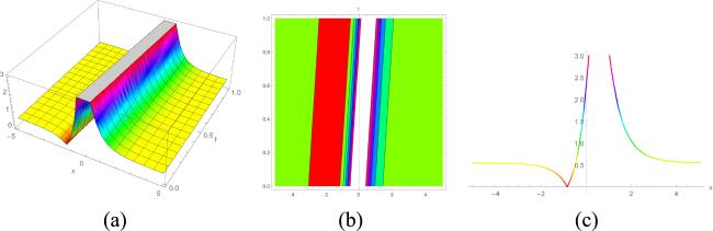
Figure 1 demonstrates the solution of $| {{ \mathcal W }}_{31}(x,t)| $ involving variables σ = 0.1, ϑ = 1, q = 0.3, γ = 0.5, τ = 0.7, S = 0.2, W = 0.61, P = 0.24, ρ = 0.32, and β = 0.21, and describes the singular soliton solution behaviour. Figure 2 also describes the periodic behaviour of solutions with variable values σ = 0.1, ϑ = 1, q = 0.3, γ = 0.5, τ = 0.7, S = 0.2, W = 0.61, P = 0.24, ρ = 0.32, and β = 0.21. Further, if we consider figure 3, it represents the singular soliton solution using parameter values σ = 0.1, ϑ = 1, q = 0.3, γ = 0.5, τ = 0.7, S = 0.2, W = 0.61, P = 0.24, ρ = 0.32, and β = 0.21. Similarly, figure 4 also represents singular soliton behaviour with parameter values σ = 1.1, ϑ = 1.1, q = 1.3, γ = 1.5, τ = 0.7, ρ = 0.32, β = 0.21, and δ = 1.41. Further discussion about figure 5 represents the V-shaped soliton solution with parameter σ = 1.1, ϑ = 1.1, q = 1.3, γ = 1.5, τ = 0.7, ρ = 0.32, β = 0.21, δ = − 0.41, and a = 0.51. Figure 6 denotes the singular soliton behaviour using variable values σ = 1.1, ϑ = 1.1, q = 1.3, γ = 1.5, τ = 0.7, rho = 0.32, β = 0.21, and δ = 0.41. Discussion regarding figure 7 demonstrates the periodic soliton behaviour with variables σ = 0.1, ϑ = 2.1, q = 0.3, γ = 0.5, τ = 0.7, S = 0.2, W = 0.61, P = 0.24, ρ = 0.32, and β = 0.21. Furthermore, figure 8 shows the bell-shaped soliton behaviour with parameter values σ = 0.1, ϑ = 1, q = 0.3, γ = 0.5, τ1 = 0.7, f = − 3.2, W = 0.61, P = 0.24, ρ = 0.32, β = 0.21, and τ = 0.23. Figure 9 represents the V-shaped soliton behaviour with variable values σ = 0.1, ϑ = 2.1, q = 0.3, γ = 0.5, τ = 0.7, P = 0.24, ρ = 0.32, and β = 0.21. Plus, figure 10 shows the periodic behaviour with variables values σ = 1.1, ϑ = 1.5, q = 1.3, γ = 1.5, τ = 1.7, S = 0.2, W = 0.61, P = 0.24, ρ = 0.32, β = 0.21. Finally, figure 11 denotes the singular soliton behaviour with parameter values σ = 1.1, ϑ = − 0.3, q = 1.3, γ = 1.5, τ = 0.7, S = 0.2, W = 0.61, P = 0.24, ρ = 0.32, and β = 0.21. To understand the solution behaviour, one can add the 3D, contour, and 2D graphics.
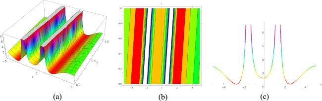
Figure 1. Graphics representation of solution $| {{ \mathcal W }}_{31}(x,t)| $ of ( |
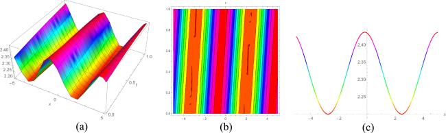
Figure 2. Graphics representation of solution $| {{ \mathcal W }}_{32}(x,t)| $ of ( |
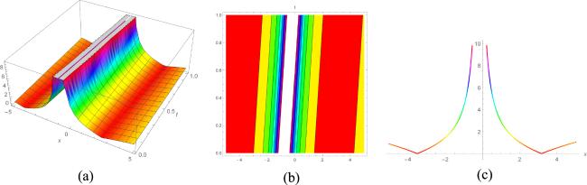
Figure 3. Graphics representation of solution $| {{ \mathcal W }}_{39}(x,t)| $ of ( |
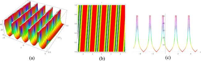
Figure 4. Graphics representation of solution $| {{ \mathcal W }}_{21}(x,t)| $ of ( |
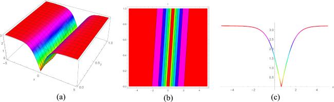
Figure 5. Graphics representation of solution $| {{ \mathcal W }}_{26}(x,t)| $ of ( |
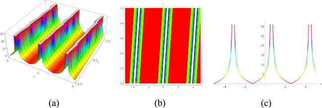
Figure 6. Graphics representation of solution $| {{ \mathcal W }}_{22}(x,t)| $ of ( |
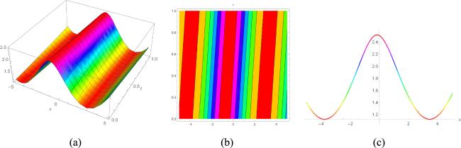
Figure 7. Graphics representation of solution $| {{ \mathcal W }}_{47}(x,t)| $ of ( |
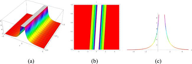
Figure 8. Graphics representation of solution $| {{ \mathcal W }}_{11}(x,t)| $ of ( |
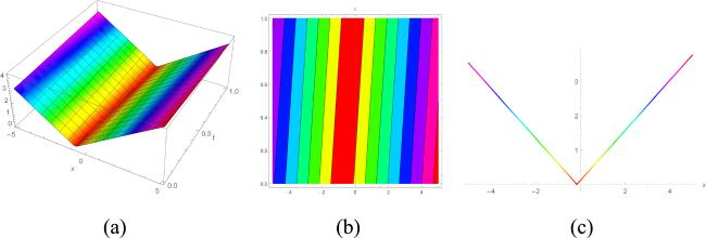
Figure 9. Graphics representation of solution $| {{ \mathcal W }}_{48}(x,t)| $ of ( |
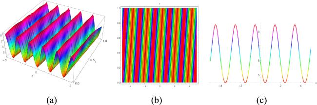
Figure 10. Graphics representation of solution $| {{ \mathcal W }}_{41}(x,t)| $ of ( |
Figure 11. Graphics representation of solution $| {{ \mathcal W }}_{40}(x,t)| $ denoting singular behaviour of ( |
6. Conclusion
In this article, the (1+1)-dimensional nonlinear chiral Schrödinger equation is studied by employing some modern analytical techniques. These approaches are of vital importance in the theory of optics and other complex models in science and engineering. Numerous travelling wave solutions for the governing model have been thoroughly explored using the applied methodologies; see figures 1–11, which illustrate the nonlinear behaviour of known results more efficiently. We are also able to attain different types of traveling-wave structures that describe the geometry of singular, periodic, V-shaped, and bell-shaped soliton solutions, which are useful to understand the dynamics of many complex models. These figures describe the attained solution behaviours. The stability analysis of the solutions have also been considered. For better understanding of solutions, some 2D, contour, and 3D graphs are visualized. In order to produce multiple new solutions for the dynamical model that appears in optical waves, the current work, to the best of our knowledge, presents a novel case study that has not been established before. It is evident from the findings that the tactics used are more capable and successful than the conventional approaches used in earlier studies. The more profound significance and dependability of the results of the investigation in explaining a wide range of physical events makes it more valuable. In future this work is highly valuable and has importance in various fields of mathematical sciences, optical fibers transmissions and physics. In the past, the applied methods in this article were not utilized in the suggested model, which explains the novelty of the work. Therefore, we can say that our findings are newly made and attained solutions are unique, robust and new. Thus, it is demonstrated that the applied approaches appear to be powerful tools in dealing with more complex higher-dimensional nonlinear evolution models that are found in advanced engineering and scientific disciplines.