


1. Introduction
Quantum gravity phenomenology predicts the possible existence of a minimal length on the smallest scale [1, 2], which suggests that the Heisenberg uncertainty principle (HUP) in quantum mechanics should be modified to use a generalized uncertainty principle (GUP) [3–8]. In this line of research, various types of GUPs [9–14] have been studied with much interest over the last few decades to extend the current understanding of general relativity (GR) to the quantum gravity regime. In particular, using the HUP and GUPs, quantum effects on classical GR have been explored through the study of Hawking radiation [15], the thermal radiation emitted by a black hole. The results heuristically include the Hawking temperature. Having obtained the Hawking temperature, one can proceed to study black holes [16–21], including their thermodynamics [22–32] and further, statistical mechanics [33–40].
However, as is well known, Einstein’s GR is the geometric theory of gravitation and a given spacetime structure is completely determined by a metric tensor as a solution to Einstein’s equations, which describe the relation between the geometry of a spacetime and the energy–momentum contained in that spacetime. In this regard, if one can find a metric tensor including the GUP effect, it would be more efficient to implement research such as black hole physics, including both classical and quantum aspects. Various authors [41–48] have tried to incorporate GUPs into metrics, which we will call a GUP-induced effective metric. Very recently, Ong [49] has obtained a satisfying GUP-induced effective metric by emphasizing the importance of using the full GUP expression instead of just series expansions [44–46], which has some subtleties and shortcomings of undesired features.
With the advent of a GUP-induced effective metric, it would be interesting to study tidal forces and their effects to see what the modification in the metric gives. In GR, it is well known that a body in free fall toward the center of another body gets stretched in the radial direction and compressed in the angular direction [50–53]. These are due to the tidal effect of gravity that causes two body parts to be stretched and/or compressed by a difference in the strength of gravity. These are common in the Universe, from our solar system to stars in binary systems, galaxies, clusters of galaxies and even gravitational waves [54]. On the theoretical side, tidal effects have been studied in various spherically symmetric spacetimes, such as the Reissner–Nordström black hole [55], the Kiselev black hole [56], some regular black holes [57, 58], the Schwarzschild black hole in massive gravity [59], the 4D Einstein–Gauss–Bonnet black hole [60], Kottler spacetimes [61], and many others [62–67].
In this paper, we study tidal effects produced in the spacetime of a Schwarzschild black hole modified by a GUP-induced effective metric. In section 2 , by following Ong’s approach, we briefly recapitulate the method to obtain a GUP-induced effective metric and study its properties. In section 3 , we investigate interesting features of the geodesic equations, and in section 4 , tidal forces for a GUP-induced Schwarzschild black hole. Then, we explicitly find radial and angular solutions of the geodesic deviation equations for radially falling bodies toward a GUP-induced Schwarzschild black hole and compare the results with the Schwarzschild solutions with no GUP effects in section 5 . A discussion is presented in section 6 .
2. GUP-induced effective metric
In this section, we briefly recapitulate Ong’s idea [49] of getting an effective metric based on a GUP, and we study the metric’s general properties. First, we begin with the most familiar form of a GUP given by
$\begin{eqnarray}{\rm{\Delta }}x{\rm{\Delta }}p\geqslant \displaystyle \frac{\hslash }{2}\,\left(1+\alpha {L}_{{\rm{p}}}^{2}\,\displaystyle \frac{{\rm{\Delta }}{p}^{2}}{{\hslash }^{2}}\right),\end{eqnarray}$
where α is a dimensionless GUP parameter of order unity and Lp is the Planck length. It is easy to see that this reduces to the HUP as α → 0. The GUP implies the following inequality $\begin{eqnarray}\begin{array}{c}\displaystyle \frac{\hslash }{\alpha {L}_{{\rm{p}}}^{2}}{\rm{\Delta }}x\,\left(1-\sqrt{1-\displaystyle \frac{\alpha {L}_{{\rm{p}}}^{2}}{{\rm{\Delta }}{x}^{2}}}\right)\leqslant {\rm{\Delta }}p\\ \,\leqslant \,\displaystyle \frac{\hslash }{\alpha {L}_{{\rm{p}}}^{2}}{\rm{\Delta }}x\,\left(1+\sqrt{1-\displaystyle \frac{\alpha {L}_{{\rm{p}}}^{2}}{{\rm{\Delta }}{x}^{2}}}\right),\end{array}\end{eqnarray}$
from which one can find that a minimum bound exists in the position uncertainty as $\begin{eqnarray}{\left({\rm{\Delta }}x\right)}_{\min }\,=\,\sqrt{\alpha }{L}_{{\rm{p}}}.\end{eqnarray}$
Now, by assuming that photons escape the Schwarzschild black hole in the radius of rH = 2M and that the spectrum of such escaping photons is thermal, according to Adler et al [16], one can arrive at the Hawking temperature
$\begin{eqnarray}{T}_{\mathrm{GUP}}\,=\,\displaystyle \frac{{Mc}}{\pi \alpha }\,\left(1-\sqrt{1-\displaystyle \frac{\alpha {\hslash }c}{4{{GM}}^{2}}}\right).\end{eqnarray}$
Here, we have followed the convention of introducing 1/2π factor to give the Hawking temperature of the Schwarzschild black hole, TSch = 1/8πM, in the small α limit. Note also that ${M}_{p}^{2}={\hslash }c/G$.On the other hand, to incorporate the GUP into a metric, by following Ong’s idea [49], one can consider a modified metric ansatz, without loss of generality, as
$\begin{eqnarray}{\rm{d}}{s}^{2}=-f\,(r)\,{\rm{d}}{t}^{2}+f{\left(\,,r\right)}^{-1}{\rm{d}}{r}^{2}+{r}^{2}{\rm{d}}{{\rm{\Omega }}}^{2}\end{eqnarray}$
with $\begin{eqnarray}f\,(r)=\left(1-\displaystyle \frac{2{GM}}{{{rc}}^{2}}\right)\,g\,(r),\end{eqnarray}$
which is the most general form of an ansatz while preserving the areal radius. Then, the Hawking temperature is modified to $\begin{eqnarray}T=\displaystyle \frac{1}{4\pi }{\left.f^{\prime} \,(r)\,\right|}_{r={r}_{H}}=\displaystyle \frac{{c}^{2}}{8\pi {GM}}g\,({r}_{H}),\end{eqnarray}$
proportional to the g(rH) function. Note that the event horizon remains intact, i.e. at rH = 2GM/c2, f(rH) = 0, although g(rH) ≠ 0.By equating the temperature in equation (2.7 ) with the GUP-induced temperature, equation (2.4 ), one can have
$\begin{eqnarray}g\,({r}_{H})=\displaystyle \frac{2{r}_{H}^{2}\,c}{G\alpha }\,\left(1-\sqrt{1-\displaystyle \frac{\alpha {L}_{{\rm{p}}}^{2}\,}{{r}_{H}^{2}}}\right),\end{eqnarray}$
where ${L}_{{\rm{p}}}^{2}=G{\hslash }/{c}^{3}$. Thus, one can infer the proper form of g(r) as $\begin{eqnarray}g\,(r)=\displaystyle \frac{2{r}^{2}c}{G\alpha }\,\left(1-\sqrt{1-\displaystyle \frac{\alpha {L}_{{\rm{p}}}^{2}}{{r}^{2}}}\right),\end{eqnarray}$
which produces an effective metric embodying the effect of the GUP as $\begin{eqnarray}\begin{array}{l}f\,(r)=\left(1-\displaystyle \frac{2{GM}}{{{rc}}^{2}}\right)\,\displaystyle \frac{2{r}^{2}c}{G\alpha }\\ \quad \times \left(1-\sqrt{1-\displaystyle \frac{\alpha {L}_{{\rm{p}}}^{2}}{{r}^{2}}}\right).\end{array}\end{eqnarray}$
For the issue of uniqueness when choosing g(r), we refer to Ong’s work [49]. Hereafter, for simplicity, we will use the Planck units of c = ℏ = G = 1, which also imply that Lp = Mp = 1. Thus, the GUP-induced effective metric which we will study has the form of $\begin{eqnarray}f\,(r)=\left(1-\displaystyle \frac{2M}{r}\right)\,\displaystyle \frac{2{r}^{2}}{\alpha }\,\left(1-\sqrt{1-\displaystyle \frac{\alpha }{{r}^{2}}}\right).\end{eqnarray}$
We have plotted the GUP-induced effective metrics with different values of α in figure 1 compared to the original Schwarzschild metric of α = 0. This graph shows that the GUP-induced effective metric functions have the same properties as the Schwarzschild case, both at the asymptotic infinity and at the event horizon. However, in between the regions of rH < r < ∞ , the curves of the GUP-induced effective metrics are slightly higher than the original Schwarzschild metric case, and when r < rH, they are lower, as shown in the inserted boxes in figure 1. In particular, since the metric in equation (2.11 ) is physically meaningful when $r\geqslant \sqrt{\alpha }$ due to the square root, the GUP parameter α makes black hole solutions possible when $\sqrt{\alpha }\lt {r}_{H}$, which was drawn in figure 2. Therefore, in this paper, we have concentrated on the GUP parameter α in the range of $0\leqslant \alpha \leqslant {r}_{H}^{2}$ to study GUP modification effects on the Schwarzschild black hole. Finally, in the small α limit, the GUP-induced effective metric is reduced to
$\begin{eqnarray}f\,(r)=\left(1-\displaystyle \frac{2M}{r}\right)\,\left(1+\displaystyle \frac{\alpha }{4{r}^{2}}+\displaystyle \frac{{\alpha }^{2}}{8{r}^{4}}\right)\end{eqnarray}$
up to α2-orders. From the second parenthesis multiplied by the original Schwarzschild metric, one may infer how much the GUP-induced effective metric differs qualitatively from the original Schwarzschild metric in the whole range of r.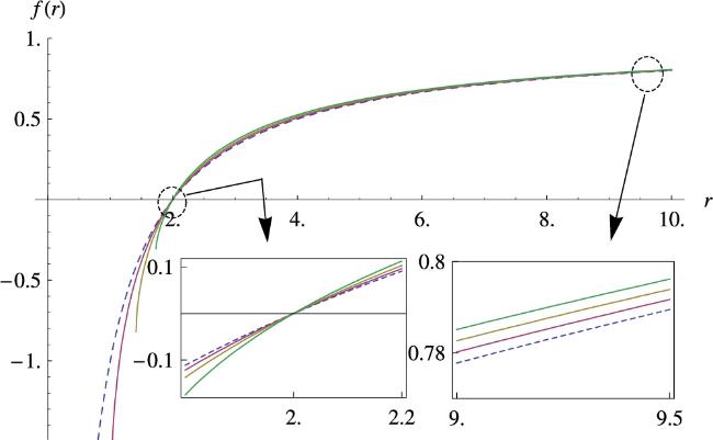
Figure 1. The effective metric: the dashed curve is for α = 0 and the solid curves are for α = 1.0, 2.0, 3.0 from down to top. Note that we have chosen M = 1 for figures unless stated otherwise. |
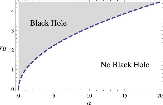
Figure 2. The plot between the event horizon rH of the black hole and the GUP parameter α in the effective metric. |
On the other hand, the Kretschmann scalar for the effective metric is given by
$\begin{eqnarray}\begin{array}{l}{K}^{2}\equiv {K}_{\mu \nu \rho \sigma }\,{K}^{\mu \nu \rho \sigma }=\displaystyle \frac{1}{{r}^{3}{\left(\,,{r}^{2}-\alpha \right)}^{2}{\alpha }^{2}}\\ \quad \times \,\left(\displaystyle \frac{{k}_{1}}{r\,({r}^{2}-\alpha )}-16{k}_{2}\,\sqrt{1-\displaystyle \frac{\alpha }{{r}^{2}}}\right),\end{array}\end{eqnarray}$
where $\begin{eqnarray}\begin{array}{l}{k}_{1}=192{r}^{10}-384{{Mr}}^{9}+32\,(8{M}^{2}-19\alpha )\,{r}^{8}\\ \quad +\,1216M\alpha {r}^{7}-8\,(96{M}^{2}-85\alpha )\,\alpha {r}^{6}-1360M{\alpha }^{2}{r}^{5}\\ \quad +\,4\,(212{M}^{2}-79\alpha )\,{\alpha }^{2}{r}^{4}+608M{\alpha }^{3}{r}^{3}\\ \quad -\,12\,(32{M}^{2}-5\alpha )\,{\alpha }^{3}{r}^{2}-96M{\alpha }^{4}r+4\,(16{M}^{2}-\alpha )\,{\alpha }^{4},\\ {k}_{2}=12{r}^{7}-24{{Mr}}^{6}+4\,(4{M}^{2}-5\alpha )\,{r}^{5}\\ \quad +\,40M\alpha {r}^{4}-8\,(3{M}^{2}-\alpha )\,\alpha {r}^{3}-16M{\alpha }^{2}{r}^{2}\\ \quad +\,(8{M}^{2}-\alpha )\,{\alpha }^{2}r+2M{\alpha }^{3}.\end{array}\end{eqnarray}$
One can find that there is no curvature singularity anywhere, except r = 0 and $r=\sqrt{\alpha }$. Note that in the limit of α → 0, the Kretschmann scalar recovers the Schwarzschild case as $\begin{eqnarray}{K}^{2}=\displaystyle \frac{48{M}^{2}}{{r}^{6}}.\end{eqnarray}$
In figure 3, we have drawn the Kretschmann scalar for the GUP-modified effective metric, showing that there is no curvature singularity, except r = 0 and $r=\sqrt{\alpha }$.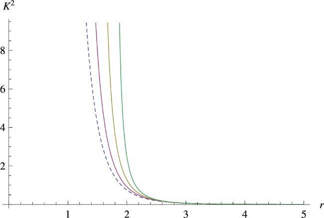
Figure 3. The Kretschmann scalar plotted over r: the dashed curve is for α = 0 and the solid curves are for α = 1.0, 2.0, 3.0 from left to right. |
3. Geodesic in Schwarzschild black hole with effective metric
Now, from the GUP-induced effective metric, equation (2.5 ) with equation (2.11 ), one can calculate the geodesic equations of3.7 ) and (3.9 ) by direct integrations as3.10 ) and (3.11 ), one can obtain
$\begin{eqnarray}\displaystyle \frac{{{\rm{d}}}^{2}{x}^{\mu }}{{\rm{d}}{\tau }^{2}}+{{\rm{\Gamma }}}_{\nu \rho }^{\mu }\,\displaystyle \frac{{\rm{d}}{x}^{\nu }}{{\rm{d}}\tau }\displaystyle \frac{{\rm{d}}{x}^{\rho }}{{\rm{d}}\tau }\,=\,0,\end{eqnarray}$
where xμ = (t, r, θ, φ). With the non-vanishing components of the Christoffel symbols $\begin{eqnarray}\begin{array}{rcl}{{\rm{\Gamma }}}_{01}^{0} & = & -{{\rm{\Gamma }}}_{11}^{1}=\displaystyle \frac{f^{\prime} \,(r)}{2f\,(r)},\,\,\,{{\rm{\Gamma }}}_{00}^{1}=\displaystyle \frac{1}{2}f^{\prime} \,(r)\,f\,(r),\\ {{\rm{\Gamma }}}_{22}^{1} & = & -{rf}\,(r),\,\,\,{{\rm{\Gamma }}}_{33}^{1}=-{rf}\,(r)\,{\sin }^{2}\;\theta ,\\ {{\rm{\Gamma }}}_{12}^{2} & = & {{\rm{\Gamma }}}_{13}^{3}=\displaystyle \frac{1}{r},\\ {{\rm{\Gamma }}}_{33}^{2} & = & -\sin \;\theta \;\cos \;\theta ,\,\,\,\,{{\rm{\Gamma }}}_{23}^{3}=\cot \;\theta ,\end{array}\end{eqnarray}$
one can explicitly obtain the geodesic equations as $\begin{eqnarray}\displaystyle \frac{{\rm{d}}{v}^{0}}{{\rm{d}}\tau }-\displaystyle \frac{\left(1-\tfrac{2M}{r}-\sqrt{1-\tfrac{\alpha }{{r}^{2}}}\right)}{r\,\left(1-\tfrac{2M}{r}\right)\,\sqrt{1-\tfrac{\alpha }{{r}^{2}}}}{v}^{0}{v}^{1}=0,\end{eqnarray}$
$\begin{eqnarray}\begin{array}{l}\displaystyle \frac{{\rm{d}}{v}^{1}}{{\rm{d}}\tau }+\displaystyle \frac{2r\,\left(1-\tfrac{2M}{r}\right)\,\left(1-\sqrt{1-\tfrac{\alpha }{{r}^{2}}}\right)\,\left(\alpha -2{r}^{2}\,\left(1-\tfrac{M}{r}\right)\,\left(1-\sqrt{1-\tfrac{\alpha }{{r}^{2}}}\right)\,\right)}{{\alpha }^{2}\sqrt{1-\tfrac{\alpha }{{r}^{2}}}}{\left(\,,{v}^{0}\right)}^{2}\\ \quad +\,\displaystyle \frac{\left(1-\tfrac{2M}{r}-\sqrt{1-\tfrac{\alpha }{{r}^{2}}}\right)}{2r\,\left(1-\tfrac{2M}{r}\right)\,\sqrt{1-\tfrac{\alpha }{{r}^{2}}}}{\left(\,,{v}^{1}\right)}^{2}\\ \quad -\,r\,\left(1-\displaystyle \frac{2M}{r}\right)\,\displaystyle \frac{2{r}^{2}}{\alpha }\,\left(1-\sqrt{1-\displaystyle \frac{\alpha }{{r}^{2}}}\right)\,[{\left({v}^{2}\right)}^{2}\\ \quad +\,{\sin }^{2}\;\theta {\left(\,,{v}^{3}\right)}^{2}]=0,\end{array}\end{eqnarray}$
$\begin{eqnarray}\displaystyle \frac{{\rm{d}}{v}^{2}}{{\rm{d}}\tau }+\displaystyle \frac{2}{r}{v}^{1}{v}^{2}-\sin \;\theta \;\cos \;\theta {\left(\,,{v}^{3}\right)}^{2}=0,\end{eqnarray}$
$\begin{eqnarray}\displaystyle \frac{{\rm{d}}{v}^{3}}{{\rm{d}}\tau }+\displaystyle \frac{2}{r}{v}^{1}{v}^{3}+2\;\cot \;\theta {v}^{2}{v}^{3}=0,\end{eqnarray}$
where we denote the four-velocity vector as vμ = dxμ/dτ. For simplicity, one can consider the geodesics on the equatorial plane θ = π/2, and thus ${v}^{2}=\dot{\theta }=0$ for all τ, without loss of generality. Then, the geodesic equations are simplified to $\begin{eqnarray}\displaystyle \frac{{\rm{d}}{v}^{0}}{{\rm{d}}\tau }-\displaystyle \frac{\left(1-\tfrac{2M}{r}-\sqrt{1-\tfrac{\alpha }{{r}^{2}}}\right)}{r\,\left(1-\tfrac{2M}{r}\right)\,\sqrt{1-\tfrac{\alpha }{{r}^{2}}}}{v}^{0}{v}^{1}=0,\end{eqnarray}$
$\begin{eqnarray}\begin{array}{l}\displaystyle \frac{{\rm{d}}{v}^{1}}{{\rm{d}}\tau }+\displaystyle \frac{2r\,\left(1-\tfrac{2M}{r}\right)\,\left(1-\sqrt{1-\tfrac{\alpha }{{r}^{2}}}\right)\,\left(\alpha -2{r}^{2}\,\left(1-\tfrac{M}{r}\right)\,\left(1-\sqrt{1-\tfrac{\alpha }{{r}^{2}}}\right)\,\right)}{{\alpha }^{2}\sqrt{1-\tfrac{\alpha }{{r}^{2}}}}{\left(\,,{v}^{0}\right)}^{2}\\ \quad +\,\displaystyle \frac{\left(1-\tfrac{2M}{r}-\sqrt{1-\tfrac{\alpha }{{r}^{2}}}\right)}{2r\,\left(1-\tfrac{2M}{r}\right)\,\sqrt{1-\tfrac{\alpha }{{r}^{2}}}}{\left(\,,{v}^{1}\right)}^{2}\\ \quad -\,r\,\left(1-\displaystyle \frac{2M}{r}\right)\,\displaystyle \frac{2{r}^{2}}{\alpha }\,\left(1-\sqrt{1-\displaystyle \frac{\alpha }{{r}^{2}}}\right)\,{\left({v}^{3}\right)}^{2}=0,\end{array}\end{eqnarray}$
$\begin{eqnarray}\displaystyle \frac{{\rm{d}}{v}^{3}}{{\rm{d}}\tau }+\displaystyle \frac{2}{r}{v}^{1}{v}^{3}=0.\end{eqnarray}$
It is now easy to find solutions for equations ( $\begin{eqnarray}{v}^{0}=\displaystyle \frac{{c}_{1}}{\left(1-\tfrac{2M}{r}\right)\,\tfrac{2{r}^{2}}{\alpha }\,\left(1-\sqrt{1-\tfrac{\alpha }{{r}^{2}}}\right)},\end{eqnarray}$
$\begin{eqnarray}{v}^{3}=\displaystyle \frac{{c}_{2}}{{r}^{2}},\end{eqnarray}$
respectively, where c1 and c2 are integration constants. Two conserved quantities defined by $\begin{eqnarray}E=-{g}_{\mu \nu }\,{\xi }^{\mu }{v}^{\nu },\end{eqnarray}$
$\begin{eqnarray}L={g}_{\mu \nu }\,{\psi }^{\mu }{v}^{\nu }\end{eqnarray}$
can be used to identify the integration constants c1, c2 with E, L, respectively. Here, ξμ = (1, 0, 0, 0) and ψμ = (0, 0, 0, 1) are the Killing vectors. Finally, by letting ds2 = − kdτ2 and using equations ( $\begin{eqnarray}\begin{array}{l}{v}^{1}=\displaystyle \frac{{\rm{d}}r}{{\rm{d}}\tau }\,=\,\pm \left[{E}^{2}-\left(k+\displaystyle \frac{{L}^{2}}{{r}^{2}}\right)\right.\\ \quad {\left.\times \,\left(1-\displaystyle \frac{2M}{r}\right)\,\displaystyle \frac{2{r}^{2}}{\alpha }\,\left(1-\sqrt{1-\displaystyle \frac{\alpha }{{r}^{2}}}\right)\,\right]}^{1/2},\end{array}\end{eqnarray}$
where the +/− sign is for outward/inward motion. Also, the timelike (null-like) geodesic is for k = 1 (0).4. Tidal force in Schwarzschild black hole with effective metric
Now, let us investigate the tidal force acting in the Schwarzschild black hole modified by the effective metric. First, let us consider the geodesic deviation equation [50–53]
$\begin{eqnarray}\displaystyle \frac{{{\rm{D}}}^{2}{\eta }^{\mu }}{{\rm{D}}{\tau }^{2}}+{R}_{\nu \rho \sigma }^{\mu }\,{v}^{\nu }{\eta }^{\rho }{v}^{\sigma }=0,\end{eqnarray}$
where ${R}_{\nu \rho \sigma }^{\mu }$ is the Riemann curvature and vμ is the unit tangent vector to the geodesic line. The geodesic deviation equation describes the behavior of a one-parameter family of neighboring geodesics through relative separation of four-vectors ημ, the infinitesimal displacement between two nearby geodesics.To study the behavior of the separation vectors in detail, we consider the timelike geodesic equation with L = 0 for simplicity. We also introduce the tetrad basis describing a freely falling frame given by
$\begin{eqnarray}\begin{array}{rcl}{e}_{\hat{0}}^{\mu } & = & \left(\displaystyle \frac{E}{f\,(r)},-\sqrt{{E}^{2}-f\,(r)},0,0\right),\\ {e}_{\hat{1}}^{\mu } & = & \left(-\displaystyle \frac{\sqrt{{E}^{2}-f\,(r)}}{f\,(r)},E,0,0\right),\\ {e}_{\hat{2}}^{\mu } & = & \left(0,0,\displaystyle \frac{1}{r},0\right),\\ {e}_{\hat{3}}^{\mu } & = & \left(0,0,0,\displaystyle \frac{1}{r\;\sin \;\theta }\right),\end{array}\end{eqnarray}$
satisfying the orthonormality relation of ${e}_{\hat{\alpha }}^{\mu }\,{e}_{\mu \hat{\beta }}\,=\,{\eta }_{\hat{\alpha }\hat{\beta }}$ with ${\eta }_{\hat{\alpha }\hat{\beta }}\,=\,\mathrm{diag}\,(-1,1,1,1)$. The separation vectors can also be expanded as ${\eta }^{\mu }={e}_{\hat{\alpha }}^{\mu }\,{\eta }^{\hat{\alpha }}$ with a fixed temporal component of ${\eta }^{\hat{0}}=0$ [51, 53].In the tetrad basis, the Riemann tensor can be written as
$\begin{eqnarray}{R}_{\hat{\beta }\hat{\gamma }\hat{\delta }}^{\hat{\alpha }}\,=\,{e}_{\mu }^{\hat{\alpha }}\,{e}_{\hat{\beta }}^{\nu }\,{e}_{\hat{\gamma }}^{\rho }\,{e}_{\hat{\delta }}^{\sigma }\,{R}_{\nu \rho \sigma }^{\mu },\end{eqnarray}$
so one can obtain the non-vanishing independent components of the Riemann tensor in the Schwarzschild black hole modified by the effective metric as $\begin{eqnarray}\begin{array}{l}{R}_{\hat{1}\hat{0}\hat{1}}^{\hat{0}}=-\displaystyle \frac{f^{\prime\prime} \,(r)}{2},\,\,{R}_{\hat{2}\hat{0}\hat{2}}^{\hat{0}}={R}_{\hat{3}\hat{0}\hat{3}}^{\hat{0}}={R}_{\hat{2}\hat{1}\hat{2}}^{\hat{1}}\\ \quad =\,{R}_{\hat{3}\hat{1}\hat{3}}^{\hat{1}}=-\displaystyle \frac{f^{\prime} \,(r)}{2r},\,\,{R}_{\hat{3}\hat{2}\hat{3}}^{\hat{2}}=\displaystyle \frac{1-f\,(r)}{{r}^{2}}.\end{array}\end{eqnarray}$
Then, one can obtain the desired tidal forces in the radially freely falling frame as $\begin{eqnarray}\begin{array}{l}\displaystyle \frac{{{\rm{d}}}^{2}{\eta }^{\hat{1}}}{{\rm{d}}{\tau }^{2}}=-\displaystyle \frac{f^{\prime\prime} \,(r)}{2}{\eta }^{\hat{1}}\\ \,=\,\displaystyle \frac{(2M-3r)\,\alpha +2{r}^{3}\,\left(1-{\left(1-\tfrac{\alpha }{{r}^{2}}\right)}^{3/2}\right)}{{r}^{3}\alpha {\,\left(1-\tfrac{\alpha }{{r}^{2}}\right)}^{3/2}}{\eta }^{\hat{1}},\end{array}\end{eqnarray}$
$\begin{eqnarray}\begin{array}{l}\displaystyle \frac{{{\rm{d}}}^{2}{\eta }^{\hat{i}}}{{\rm{d}}{\tau }^{2}}=-\displaystyle \frac{f^{\prime} \,(r)}{2r}{\eta }^{\hat{i}}\\ \,=\,-\displaystyle \frac{\alpha +2\,(M-r)\,r\,\left(1-\sqrt{1-\tfrac{\alpha }{{r}^{2}}}\right)}{{r}^{2}\alpha \sqrt{1-\tfrac{\alpha }{{r}^{2}}}}{\eta }^{\hat{i}},\end{array}\end{eqnarray}$
where i = 2, 3. As α → 0, they are reduced to $\begin{eqnarray}\displaystyle \frac{{{\rm{d}}}^{2}{\eta }^{\hat{1}}}{{\rm{d}}{\tau }^{2}}=\displaystyle \frac{2M}{{r}^{3}}{\eta }^{\hat{1}},\end{eqnarray}$
$\begin{eqnarray}\displaystyle \frac{{{\rm{d}}}^{2}{\eta }^{\hat{i}}}{{\rm{d}}{\tau }^{2}}=-\displaystyle \frac{M}{{r}^{3}}{\eta }^{\hat{i}},\end{eqnarray}$
which are the radial and angular tidal forces of the Schwarzschild black hole. As a result, we have newly obtained the tidal effect that is dependent on the GUP parameter α that is embodied in the effective metric. In figure 4, we have plotted the radial and angular tidal forces by comparing them with the original Schwarzschild case.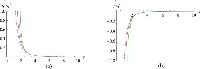
Figure 4. (a) Radial and (b) angular tidal forces with different GUP parameters α = 1.0, 2.0, 3.0 from the left. The dashed curves are for α = 0, the original Schwarzschild case. |
As seen in figure 4(a), the radial tidal forces are always positive, and as the GUP parameters α increase, the curves move to the right while the curves' shapes remain the same. It seems appropriate to comment that the radial tidal forces go to infinities as they approach their singularities; therefore, the radial stretchings get infinities. A similar interpretation can be applied to the angular tidal forces. However, note that they go to negative infinities as r approaches the singularity, as seen in figure 4(b). Thus, there are infinite compressions in the angular direction.
5. Geodesic deviation equations of Schwarzschild black hole with effective metric
For the geodesic deviation equations (4.5 ) and (4.6 ) of the Schwarzschild black hole modified by the effective metric, the tidal forces can be rewritten in terms of the r-derivative as5.1 ), is known to have the following general form of5.2 ), it is
$\begin{eqnarray}[{E}^{2}-f\,(r)]\,\displaystyle \frac{{{\rm{d}}}^{2}{\eta }^{\hat{1}}}{{\rm{d}}{r}^{2}}-\displaystyle \frac{f^{\prime} \,(r)}{2}\displaystyle \frac{{\rm{d}}{\eta }^{\hat{1}}}{{\rm{d}}r}+\displaystyle \frac{f^{\prime\prime} \,(r)}{2}{\eta }^{\hat{1}}=0,\end{eqnarray}$
$\begin{eqnarray}[{E}^{2}-f\,(r)]\,\displaystyle \frac{{{\rm{d}}}^{2}{\eta }^{\hat{i}}}{{\rm{d}}{r}^{2}}-\displaystyle \frac{f^{\prime} \,(r)}{2}\displaystyle \frac{{\rm{d}}{\eta }^{\hat{i}}}{{\rm{d}}r}+\displaystyle \frac{f^{\prime} \,(r)}{2r}{\eta }^{\hat{i}}=0.\end{eqnarray}$
The solution of the radial component, equation ( $\begin{eqnarray}\begin{array}{l}{\eta }^{\hat{1}}\,(r)={c}_{1}\,\sqrt{{E}^{2}-f\,(r)}+{c}_{2}\,\sqrt{{E}^{2}-f\,(r)}\\ \,\times \displaystyle \int \displaystyle \frac{{\rm{d}}r}{{\left[{E}^{2}-f\,(r)\right]}^{3/2}},\end{array}\end{eqnarray}$
and for the angular component, equation ( $\begin{eqnarray}{\eta }^{\hat{i}}\,(r)=r\,\left({c}_{3}+{c}_{4}\,\int \displaystyle \frac{{\rm{d}}r}{{r}^{2}\sqrt{{E}^{2}-f\,(r)}}\right),\end{eqnarray}$
where ci (i = 1, 2, 3, 4) are constants of integration [55–61], which will be determined by the boundary conditions.Now, let us solve the geodesic deviation equations (5.1 ) and (5.2 ) by series expansions of the integrands to the power of α. Firstly, we consider a body released from rest at r = b so that we have $E=\sqrt{f\,(b)}$. Then, the term E2 − f(r) can be expressed as5.1 ), can be obtained up to α2 order as
$\begin{eqnarray}{E}^{2}-f\,(r)=2M\,\left(\displaystyle \frac{1}{r}-\displaystyle \frac{1}{b}\right)\,Q\,(r),\end{eqnarray}$
where $\begin{eqnarray}\begin{array}{rcl}Q\,(r) & = & 1+\displaystyle \sum _{n=1}^{\infty }\,{\alpha }^{n}\displaystyle \frac{(2n-1)\,!!}{(n+1)!{2}^{n}}\\ & & \times \,\left(-\displaystyle \frac{{P}_{n}\,(r)}{2M}+{P}_{n+1}\,(r)\right),\\ & \equiv & 1+\displaystyle \sum _{n=1}^{\infty }\,{\alpha }^{n}{Q}^{(n)\,}(r),\\ {P}_{n}\,(r) & = & \displaystyle \sum _{m=0}^{n}\,\displaystyle \frac{1}{{r}^{n-m}{b}^{m}}.\end{array}\end{eqnarray}$
Here, Q(n)(r) is the function of r of order αn. Then, without loss of generality, the solution of the radial component, equation ( $\begin{eqnarray}\begin{array}{l}{\eta }^{\hat{1}}\,(r)={c}_{1}\,\sqrt{\displaystyle \frac{2M}{b}}\displaystyle \frac{\sqrt{{br}-{r}^{2}}}{r}\sqrt{1+\alpha {Q}^{(1)\,}(r)+{\alpha }^{2}{Q}^{(2)\,}(r)}\\ \quad +\,{c}_{2}\,\displaystyle \frac{b}{2M}\sqrt{1+\alpha {Q}^{(1)\,}(r)+{\alpha }^{2}{Q}^{(2)\,}(r)}\\ \quad \times \,\left[2{{bd}}_{1}\,(r)+\displaystyle \frac{3b}{2r}{d}_{2}\,(r)\,\sqrt{{br}-{r}^{2}}{\;\cos }^{-1}\;\,\left(\displaystyle \frac{2r}{b}-1\right)\,\right],\end{array}\end{eqnarray}$
$\begin{eqnarray}{\eta }^{\hat{i}}\,(r)={c}_{3}\,r-{c}_{4}\,\sqrt{\displaystyle \frac{2b}{M}}\displaystyle \frac{\sqrt{{br}-{r}^{2}}}{b}{d}_{3}\,(r),\end{eqnarray}$
where $\begin{eqnarray}\begin{array}{l}{d}_{1}\,(r)=\displaystyle \frac{3}{2}-\displaystyle \frac{r}{2b}+\displaystyle \frac{3\alpha }{16b}\,\left(\displaystyle \frac{5}{2M}-\displaystyle \frac{7}{b}+\displaystyle \frac{r}{{b}^{2}}-\displaystyle \frac{r}{2{bM}}\right)\\ \quad +\,\displaystyle \frac{3{\alpha }^{2}}{64{b}^{2}r}\,\left(\displaystyle \frac{1}{b}+\displaystyle \frac{1}{2M}+\displaystyle \frac{1}{2r}+\displaystyle \frac{r}{4{b}^{2}}+\displaystyle \frac{45r}{16{M}^{2}}\right.\\ \quad \left.-\,\displaystyle \frac{31r}{4{bM}}+\displaystyle \frac{3{r}^{2}}{4{b}^{3}}-\displaystyle \frac{5{r}^{2}}{16{{bM}}^{2}}+\displaystyle \frac{{r}^{2}}{4{b}^{2}M}\right),\\ {d}_{2}\,(r)=1+\displaystyle \frac{5\alpha }{8b}\,\left(\displaystyle \frac{1}{2M}-\displaystyle \frac{1}{b}\right)\\ \quad +\,\displaystyle \frac{5{\alpha }^{2}}{128{b}^{2}}\,\left(\displaystyle \frac{7}{4{M}^{2}}-\displaystyle \frac{3}{{bM}}-\displaystyle \frac{1}{{b}^{2}}\right),\\ {d}_{3}\,(r)=1+\displaystyle \frac{\alpha }{8}\,\left(\displaystyle \frac{5}{6{Mb}}-\displaystyle \frac{11}{5{b}^{2}}+\displaystyle \frac{1}{6{Mr}}-\displaystyle \frac{3}{5{br}}-\displaystyle \frac{1}{5{r}^{2}}\right)\\ \quad +\,\displaystyle \frac{{\alpha }^{2}}{16}\,\left(\displaystyle \frac{43}{160{b}^{2}{M}^{2}}-\displaystyle \frac{33}{280{b}^{3}M}-\displaystyle \frac{551}{504{b}^{4}}+\displaystyle \frac{7}{80{{bM}}^{2}r}\right.\\ \quad -\,\displaystyle \frac{17}{140{b}^{2}{Mr}}-\displaystyle \frac{59}{252{b}^{3}r}+\displaystyle \frac{3}{160{M}^{2}{r}^{2}}-\displaystyle \frac{1}{35{{bMr}}^{2}}\\ \quad \left.-\,\displaystyle \frac{19}{168{b}^{2}{r}^{2}}+\displaystyle \frac{1}{56{{Mr}}^{3}}-\displaystyle \frac{29}{252{{br}}^{3}}-\displaystyle \frac{5}{72{r}^{4}}\right).\end{array}\end{eqnarray}$
Note that d2(r) has no r-dependence. The integration constants ci can be determined by adopting appropriate boundary conditions where the infinitesimal displacement and initial velocity between two nearby particles are given by ηk(b) and dηk(r)/dτ∣r=b ≡ dηk(b)/dτ (k = 1, 2, 3) at r = b. Explicitly, we have $\begin{eqnarray}\begin{array}{rcl}{c}_{1} & = & \displaystyle \frac{{b}^{2}}{M}{\left(\,,1+\alpha {Q}^{(1)\,}(b)+{\alpha }^{2}{Q}^{(2)\,}(b)\right)}^{-1}\displaystyle \frac{{\rm{d}}{\eta }^{\hat{1}}\,(b)}{{\rm{d}}\tau },\\ {c}_{2} & = & \displaystyle \frac{M}{{b}^{2}}{\left(\,,1+\alpha {Q}^{(1)\,}(b)+{\alpha }^{2}{Q}^{(2)\,}(b)\right)}^{-1/2}{d}_{1}^{-1}\,(b)\,{\eta }^{\hat{1}}\,(b),\\ {c}_{3} & = & \displaystyle \frac{1}{b}{\eta }^{\hat{i}}\,(b),\\ {c}_{4} & = & -b{\left(\,,1+\alpha {Q}^{(1)\,}(b)+{\alpha }^{2}{Q}^{(2)\,}(b)\right)}^{-1/2}{d}_{3}^{-1}\,(b)\,\displaystyle \frac{{\rm{d}}{\eta }^{\hat{i}}\,(b)}{{\rm{d}}\tau }.\end{array}\end{eqnarray}$
Thus, the solutions are finally written as $\begin{eqnarray}\begin{array}{rcl}{\eta }^{\hat{1}}\,(r) & = & b\sqrt{\displaystyle \frac{2b}{M}}\displaystyle \frac{{\rm{d}}{\eta }^{\hat{1}}\,(b)}{{\rm{d}}\tau }\displaystyle \frac{\sqrt{{br}-{r}^{2}}}{r}\\ & & \times \,\displaystyle \frac{{\left(1+\alpha {Q}^{(1)\,}(r)+{\alpha }^{2}{Q}^{(2)\,}(r)\right)}^{1/2}}{\left(1+\alpha {Q}^{(1)\,}(b)+{\alpha }^{2}{Q}^{(2)\,}(b)\right)}\\ & & +\,{\eta }^{\hat{1}}\,(b)\,{d}_{1}^{-1}\,(b)\,{\left(\displaystyle \frac{1+\alpha {Q}^{(1)\,}(r)+{\alpha }^{2}{Q}^{(2)\,}(r)}{1+\alpha {Q}^{(1)\,}(b)+{\alpha }^{2}{Q}^{(2)\,}(b)}\right)}^{1/2}\\ & & \times \,\left[{d}_{1}\,(r)+\displaystyle \frac{3}{4r}{d}_{2}\,(r)\,\sqrt{{br}-{r}^{2}}{\;\cos }^{-1}\;\,\left(\displaystyle \frac{2r}{b}-1\right)\,\right],\end{array}\end{eqnarray}$
$\begin{eqnarray}\begin{array}{c}{\eta }^{\hat{i}}\,(r)=\displaystyle \frac{1}{b}{\eta }^{\hat{i}}\,(b)\,r+\sqrt{\displaystyle \frac{2b}{M}}\displaystyle \frac{\left.{\rm{d}}{\eta }^{\hat{i}}\,(b\right)}{{\rm{d}}\tau }{d}_{2}^{-1}\,(b)\\ \,\times \,{\left(\displaystyle \frac{{br}-{r}^{2}}{1+\alpha {Q}^{\left(1\,\right)}\left(\,b)+{\alpha }^{2}{Q}^{\left(2\,\right)}\,(b\right)}\right)}^{1/2}{d}_{3}\,(r).\end{array}\end{eqnarray}$
In figure 5, we have drawn the radial components of the geodesic deviation by comparing the case of not having a GUP parameter to that of having a GUP parameter for both $\tfrac{{\rm{d}}{\eta }^{\hat{1}}\,(b)}{{\rm{d}}\tau }\,=\,0$ and $\tfrac{{\rm{d}}{\eta }^{\hat{1}}\,(b)}{{\rm{d}}\tau }\ne 0$ initial velocities. From the figure, one can see that the radial separation vectors of a falling object in the GUP-modified Schwarzschild black hole start with the same initial values as the original Schwarzschild black hole, and then it gets stretched steeper than the original Schwarzschild case as it approaches the singularities. This results in much greater separation effects. Note that when comparing figures 5(a) and (b), the latter shows a much steeper slope in the range of 0 < r < 10 than the former. In figure 6, we have also drawn the radial components of the geodesic deviation by varying the mass parameter M in the Schwarzschild black hole modified by the effective metric. Here, one can find that the bigger the black hole mass is, the greater the geodesic separation is near the singularity. Moreover, for comparison, we have drawn the radial components of geodesic deviation for the Planck mass comparable scales M in figure 6(a) and for some larger M in figure 6(b), which shows that the latter sharply increases compared to the former as it approaches the singularity.
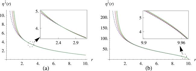
Figure 5. Radial components of geodesic deviation in the Schwarzschild black hole modified by an effective metric, (a) with $\tfrac{{\rm{d}}{\eta }^{\hat{1}}(b)}{{\rm{d}}\tau }\,=\,0$, and (b) with $\tfrac{{\rm{d}}{\eta }^{\hat{1}}(b)}{{\rm{d}}\tau }\,=\,1\,(\ne 0)$: the dashed curves are for α = 0, and the solid curves for α = 1.0, 2.0, 3.0 from the left. |
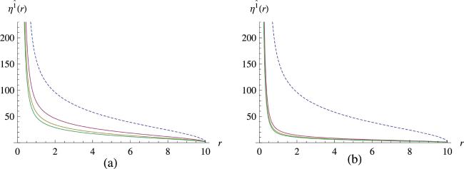
Figure 6. Radial components of geodesic deviation by varying the mass M in the Schwarzschild black hole modified by an effective metric with $\tfrac{{\rm{d}}{\eta }^{\hat{1}}(b)}{{\rm{d}}\tau }\,=\,1$: (a) the solid curves for M = 5, 10, 15, and (b) the solid curves for M = 100, 200, 300, downwards, with the dashed curve for M = 1. |
Meanwhile, in figure 7, we have drawn the angular components of the geodesic deviation in the Schwarzschild black hole modified by the α-dependent effective metric. Figure 7(a) corresponds to α = 0 with zero initial velocity, $\tfrac{{\rm{d}}{\eta }^{\hat{1}}\,(b)}{{\rm{d}}\tau }\,=\,0$, the original Schwarzschild case. When the initial velocity of the original Schwarzschild black hole is non-zero as $\tfrac{{\rm{d}}{\eta }^{\hat{1}}\,(b)}{{\rm{d}}\tau }\ne 0$, the angular separation is drawn by the dashed curve in figure 7(b). Now, the angular components of the geodesic deviation in the Schwarzschild black hole modified by an effective metric by varying the GUP parameter α are drawn by the solid curves in figure 7(b). Note that as the GUP parameters α increase, the angular separation appears to be larger in all ranges, except near the singularity, where the angular separation is inverted to be small. Moreover, in figure 8, we have also drawn the angular components of the geodesic deviation by varying the mass. The original Schwarzschild case is drawn in figure 8(a). The GUP-modified Schwarzschild black hole case is drawn in figure 8(b), which shows that it resembles the original Schwarzschild case but differs near the singularities. Moreover, for comparison, for some large M cases, we have drawn the angular components of geodesic deviation in figure 9, which shows the angular separations have not changed much.

Figure 7. Angular components of geodesic deviation in the Schwarzschild black hole modified by the α-dependent effective metric: (a) with α = 0 and $\tfrac{{\rm{d}}{\eta }^{\hat{1}}(b)}{{\rm{d}}\tau }\,=\,0$, (b) with α = 0 and $\tfrac{{\rm{d}}{\eta }^{\hat{1}}(b)}{{\rm{d}}\tau }\,=\,1$ for the dashed curve, and α = 1.0, 2.0, 3.0 (from the left near r = 0.5) and $\tfrac{{\rm{d}}{\eta }^{\hat{1}}(b)}{{\rm{d}}\tau }\,=\,1$ for the solid curves. |
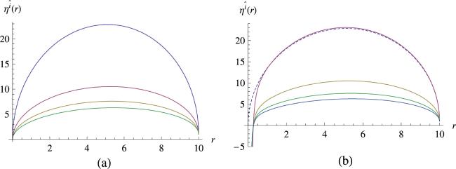
Figure 8. (a) Angular components of geodesic deviation by varying the mass M in the effective metric for M = 1, 5, 10, 15 (from top to down) with α = 0 in the original Schwarzschild black hole. (b) Angular components of geodesic deviation by varying the mass in the effective metric for M = 1, 5, 10, 15 with α = 1 in the Schwarzschild black hole modified by an effective metric. Here, the dashed curve is for the α = 0 case, drawn for comparison. |

Figure 9. (a) Angular components of geodesic deviation by varying the mass M in the effective metric for M = 1, 100, 200, 300 (from top to down) with α = 0 in the original Schwarzschild black hole. (b) Angular components of geodesic deviation by varying the mass in the effective metric for M = 1, 100, 200, 300 with α = 1 in the Schwarzschild black hole modified by an effective metric. Here, the dashed curve is for the α = 0 case, as before, drawn for comparison. |
It seems appropriate to comment that as it approaches the singularity, the radial and angular components of the geodesic deviation of the GUP-modified Schwarzschild black hole are stretched steeper and larger than those of the original Schwarzschild black hole, respectively. It looks peculiar since we usually expect quantum gravity effects such as a GUP to make physical quantities more finite, not worse. However, there is also an example of applying GUP to white dwarfs, which leads to a peculiar property. A GUP can remove the Chandrasekhar limit [68–70], and thus white dwarfs can be seemingly arbitrarily large. In this respect, a GUP correction can lead to more divergent behavior for some physical quantities, which goes against our usual expectations and should be further studied.
6. Discussion
In this paper, we have studied tidal effects in a GUP-effect embodied Schwarzschild black hole. We have first recapitulated the GUP-induced effective metric by following Ong’s approach and have studied its properties in detail. As a result, we have shown that the α-dependent effective metric is only valid in the $0\leqslant \alpha \leqslant {r}_{H}^{2}$ range. When $\alpha \gt {r}_{H}^{2}$, it does not even form an event horizon. Moreover, we have also obtained the Kretschmann scalar for the effective metric, showing no curvature singularity, except r = 0 and $r=\sqrt{\alpha }$.
Then, we have investigated interesting features of the geodesic equations and tidal forces that are dependent on the GUP parameter α. By comparing the radial and angular tidal forces with the original Schwarzschild case, we have shown that as the GUP parameters α increase, the radial and angular tidal forces go to infinities faster than those of the original Schwarzschild black hole’s.
Furthermore, by considering a free fall of a body released from rest at r = b, we have derived the geodesic deviation equations and explicitly and analytically solved them. As a result, we have shown that the radial components of the geodesic deviation get stretched steeper than the original Schwarzschild case when approaching the singularities, resulting in much greater separation effects. Also, by varying the mass parameter M, we have found that the bigger the black hole mass is, the greater the geodesic separation is near the singularity. On the other hand, as the GUP parameters α increase, the curves of the angular components of the geodesic deviation are higher over almost all ranges r < b, and then they become lower near the singularity than the original Schwarzschild case. As a result, we have found that the α-dependent effective metric affects both the radial and angular components, particularly near the singularities, compared with the original Schwarzschild black hole case.
Finally, it seems appropriate to comment that our coordinate systems still contain a singularity at $r=\sqrt{\alpha }$, implying that the geodesics are still incomplete inside the black hole. In this respect, it would be interesting to construct and analyze the tidal effect, related to the works of [71–74], on GUP-induced geodesically compete non-singular black holes through further investigation.