


1. Introduction
Gravitational effects can be manifested through three different avenues. In general relativity, the space–time curvature describes the gravity. In teleparallel and symmetric teleparallel theories of general relativity, the gravitational effects are ascribed to torsion and nonmetricity, respectively. The symmetric teleparallel f(Q) theory of gravity has been at the center of extensive study for quite some time now. With the help of data from various astrophysical observations such as Type Ia supernovae (SNe Ia) and quasars, Lazkoz et al [1] analyzed the validity of the f(Q) theory. The validity of f(Q) cosmological models has also been investigated [2] through the embedding approach. D’Ambrosio et al [3] studied black holes (BHs) in f(Q) gravity. The static and spherically symmetric solutions resulting from f(Q) gravity immersed in an anisotropic fluid were elucidated in [4]. Hassan et al [5] analyzed wormhole geometries in f(Q) gravity, employing the linear equation of state and anisotropic solutions. Mustafa et al [6] elucidated the possibility of traversal wormholes consistent with energy conditions. There have been various studies regarding wormholes in f(Q) gravity [7, 8]. Calza and Sebastiani [9] scrutinized various aspects of static and spherically symmetric solutions in f(Q) gravity.
Observations of various astrophysical phenomena provide an excellent avenue for probing different theories of gravity. One such phenomenon is the quasinormal modes (QNMs) of BHs. Since QNMs bear imprints of the underlying space–time, they can be utilized to obtain important aspects of space–time. These modes are referred to as quasinormal because, unlike normal modes, they are transient in nature. These modes represent oscillations of the BH that eventually die out owing to the emission of gravitational waves. QNMs are basically complex-valued numbers where the real part provides the frequency of the emitted gravitational waves and the imaginary part gives the decay rate or the damping rate. BHs undergo three different phases after perturbation: inspiral, merger and ringdown. QNMs are related to the ringdown phase for remnant BHs. A significant number of articles have studied QNMs of various black holes [10–43]. Jha [44, 45] has studied QNMs of non-rotating loop quantum gravity and Simpson–Visser BHs, respectively. Gogoi et al [46] studied QNMs of a static and spherically symmetric BH in f(Q) gravity for scalar and electromagnetic fields. In this article, we intend to study QNMs of the BH for a massless Dirac field and investigate its time evolution and will not discuss the relevant material in [46].
Another astrophysical phenomenon that encodes important information about the underlying space–time is gravitational lensing. In the absence of any massive object, light rays travel in a straight line. But in the presence of BHs, due to their strong gravitational fields, light rays become deflected. Thus, BHs act as gravitational lenses. Since the deflection angle is a function of different parameters that arise in the theory of gravity under consideration, the study of gravitational lensing provides us with a way to analyze the effect of various theories of gravity on the observable. The phenomenon of gravitational lensing has been studied extensively in strong as well as weak field limits in various articles [47–75]. Motivated by previous studies, and with the intention of studying the effect of the nonmetricity parameter on the deflection angle, we study gravitational lensing in f(Q) gravity in the weak field limit.
Our primary focus in this article is to gauge the impact of the nonmetricity scalar Q0 on astrophysical observations such as QNMs and gravitational lensing. It is imperative to probe the signature of additional parameter(s) so that with future experimental results we can either validate or invalidate the new solution. The structure of the paper is as follows: section 2 briefly discusses the space–time of a static and spherical BH in f(Q) gravity. In section 3 we describe the massless Dirac perturbation at the neighborhood of a static BH in f(Q) gravity. In section 4 the QNM frequencies are evaluated using the sixth-order Wentzel–Kramers–Brillouin (WKB) method. The time evolution profile of the Dirac perturbation is provided in section 5 . In section 6 we study the deflection angle in the weak field limit. We end our manuscript with a brief discussion of the results.
2. A brief discussion on a static BH in f(Q) gravity
The action for f(Q) gravity is [76]1 ) with respect to the metric gμν gives the field equation1 ) with respect to the connection, one obtains9 ) implies that7 ) results in14 ) as follows:16 ), it is obvious that this BH has a physical singularity at r = 0, and that the nonmetricity scalar Q0 considerably alters the scalars associated with this BH.
$\begin{eqnarray}S=\int \sqrt{-g}{\rm{d}}{x}^{4}\left(\displaystyle \frac{1}{2}f\left(Q\right)+{L}_{m}\right),\end{eqnarray}$
where g is the determinant of the metric gμν, f(Q) is an arbitrary function of the nonmetricity Q and Lm is the matter Lagrangian density. Varying the action ( $\begin{eqnarray}\begin{array}{l}-{T}_{\mu \nu }=\displaystyle \frac{2}{\sqrt{-g}}{{\rm{\nabla }}}_{\alpha }\left(\sqrt{-g}\displaystyle \frac{\partial f}{\partial Q}{P}_{\mu \nu }^{\alpha }\right)+\displaystyle \frac{1}{2}{g}_{\mu \nu }f\\ \,+\displaystyle \frac{\partial f}{\partial Q}\left({P}_{\mu \alpha \beta }{Q}_{\nu }^{\alpha \beta }-2{Q}_{\alpha \beta \mu }{P}_{\nu }^{\alpha \beta }\right).\end{array}\end{eqnarray}$
The stress–energy momentum tensor for cosmic matter content is determined by $\begin{eqnarray}{T}_{\mu \nu }\equiv \displaystyle \frac{-2}{\sqrt{-g}}\displaystyle \frac{\delta \left(\sqrt{-g}{L}_{m}\right)}{\delta {g}^{\mu \nu }}.\end{eqnarray}$
Varying equation ( $\begin{eqnarray}{\rm{\nabla }}\mu {{\rm{\nabla }}}_{\nu }\left(\sqrt{-g}\displaystyle \frac{\partial f}{\partial Q}{P}_{\alpha }^{\mu \nu }\right)=0.\end{eqnarray}$
The metric ansatz for a generic static and spherically symmetric space–time is written as $\begin{eqnarray}{\rm{d}}{s}^{2}=-{{\rm{e}}}^{a\left(r\right)}{\rm{d}}{t}^{2}+{{\rm{e}}}^{b\left(r\right)}{\rm{d}}{r}^{2}+{r}^{2}\left({\rm{d}}{\theta }^{2}+{\sin }^{2}\theta {\rm{d}}{\phi }^{2}\right).\end{eqnarray}$
For this ansatz, the nonmetricity scalar Q can be written as [77] $\begin{eqnarray}Q\left(r\right)=\displaystyle \frac{2{{\rm{e}}}^{b\left(r\right)}}{r}\left({a}^{{\prime} }+\displaystyle \frac{1}{r}\right),\end{eqnarray}$
where the prime $\left({}^{{\prime} }\right)$ denotes a derivative with respect to the radial coordinate r. For a constant nonmetricity scalar $\left(Q={Q}_{0}\right),$ the above equation can be written as $\begin{eqnarray}{a}^{{\prime} }\left(r\right)=-\displaystyle \frac{{Q}_{0}{{r}{\rm{e}}}^{b\left(r\right)}}{2}-\displaystyle \frac{1}{r}.\end{eqnarray}$
Following [77], the components of the field equation in the case of a vacuum can be written as $\begin{eqnarray}\displaystyle \frac{\partial f\left({Q}_{0}\right)}{\partial Q}\displaystyle \frac{{{\rm{e}}}^{-b}}{r}\left({a}^{{\prime} }+{b}^{{\prime} }\right)=0,\end{eqnarray}$
$\begin{eqnarray}\displaystyle \frac{f\left({Q}_{0}\right)}{2}+\displaystyle \frac{\partial f\left({Q}_{0}\right)}{\partial Q}\left({Q}_{0}+\displaystyle \frac{1}{{r}^{2}}\right)=0,\end{eqnarray}$
$\begin{eqnarray}\begin{array}{l}\displaystyle \frac{\partial f\left({Q}_{0}\right)}{\partial Q}\left[\displaystyle \frac{{Q}_{0}}{2}+\displaystyle \frac{1}{{r}^{2}}+{{\rm{e}}}^{-b}\left(\displaystyle \frac{{a}^{{\prime\prime} }}{2}\right.\right.\\ \left.\left.\,+\left(\displaystyle \frac{{a}^{{\prime} }}{4}+\displaystyle \frac{1}{2r}\right)\left({a}^{{\prime} }-{b}^{{\prime} }\right)\right)\right]=0.\end{array}\end{eqnarray}$
Equation ( $\begin{eqnarray}f\left({Q}_{0}\right)=0,\qquad \displaystyle \frac{\partial f\left({Q}_{0}\right)}{\partial Q}=0.\end{eqnarray}$
Those two conditions imply that $\begin{eqnarray}f(Q)=\displaystyle \sum _{n}{a}_{n}{\left(Q-{Q}_{0}\right)}^{n},\end{eqnarray}$
where an represents arbitrary model parameters. Assume ${{\rm{e}}}^{a\left(r\right)}=1-2M/r$ then equation ( $\begin{eqnarray}{{\rm{e}}}^{b}=\displaystyle \frac{-2}{{Q}_{0}r\left(r-2M\right)}.\end{eqnarray}$
The metric of the static spherical BH in f(Q) gravity is given by [77] $\begin{eqnarray}{\rm{d}}{s}^{2}=f(r){\rm{d}}{t}^{2}-\displaystyle \frac{1}{g(r)}{\rm{d}}{r}^{2}-{r}^{2}\left({\rm{d}}{\theta }^{2}+{\sin }^{2}\theta {\rm{d}}{\phi }^{2}\right)\end{eqnarray}$
where $\begin{eqnarray}f\left(r\right)=1-\displaystyle \frac{2M}{r},\qquad g(r)=\displaystyle \frac{-{Q}_{0}{r}^{2}}{2}\left(1-\displaystyle \frac{2M}{r}\right),\end{eqnarray}$
in which, M is the BH mass and Q0 is the constant nonmetricity scalar which must have Q0 < 0. In contrast to a Schwarzschild BH, this BH has a nonmetricity scalar Q0. Moreover, it modifies the scalars of metric ( $\begin{eqnarray}\begin{array}{l}R=\displaystyle \frac{3\left(r-M\right){Q}_{0}r+2}{{r}^{2}}\to \mathrm{Ricci}\,\mathrm{scalar}\\ {R}_{\mu \nu }{R}^{\mu \nu }=\displaystyle \frac{\left(9{M}^{2}-14{Mr}+6{r}^{2}\right){Q}_{0}^{2}{r}^{2}+8\left(r-M\right){Q}_{0}r+4}{2{r}^{4}}\to \mathrm{Ricci}\ \mathrm{squared}\ \mathrm{scalar},\\ { \mathcal K }=\displaystyle \frac{\left(9{M}^{2}-8{Mr}+3{r}^{2}\right){Q}_{0}^{2}{r}^{2}+4\left(r-2M\right){Q}_{0}r+4}{{r}^{4}}\to \mathrm{Kretchmann}\,\mathrm{scalar}.\end{array}\end{eqnarray}$
According to equation (The Hawking temperature of the metric (14 ) can be calculated using the surface gravity given by [78]14 ) reads18 ), it is obvious that the nonmetricity scalar Q0 increases the Hawking temperature of the static BH. The behavior of the Hawking temperature is plotted in figure 1.
$\begin{eqnarray}\kappa ={{\rm{\nabla }}}_{\mu }{\chi }^{\mu }{{\rm{\nabla }}}_{\nu }{\chi }^{\nu },\end{eqnarray}$
where χμ is the timelike Killing vector field. Therefore, the Hawking temperature of the static BH ( $\begin{eqnarray}\begin{array}{l}{T}_{{BH}}=\displaystyle \frac{1}{4\pi \sqrt{-{g}_{{tt}}{g}_{{rr}}}}{\left.\displaystyle \frac{{{\rm{d}}{g}}_{{tt}}}{{\rm{d}}{r}}\right|}_{r={r}_{h}}=\displaystyle \frac{1}{4\pi \sqrt{-\tfrac{2}{{Q}_{0}{r}^{2}}}}\displaystyle \frac{2M}{{r}^{2}}\\ \,=\,\displaystyle \frac{1}{4\pi }\sqrt{-\displaystyle \frac{{Q}_{0}}{2}}.\end{array}\end{eqnarray}$
From equation (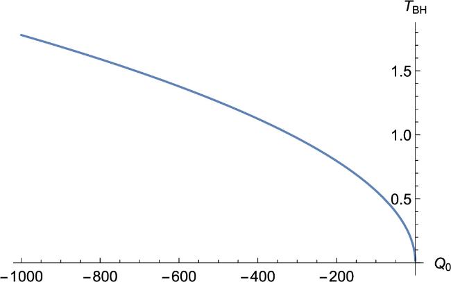
Figure 1. Hawking temperature versus Q0. |
3. Massless Dirac perturbation
In this section, we will discuss the massless Dirac perturbation in a static and spherical BH in f(Q) gravity. To study the massless spin-1/2 field, we will use the Newman–Penrose formalism [79]. The Dirac equations [80] are given by14 ) is19 ) yields a single equation of motion for F1 only (which is actually the equation of motion for a massless Dirac field)20 ) and (21 ), we can express equation (22 ) explicitly as23 ) into radial and angular parts, we consider the spin-1/2 wave function in the form of23 ) becomes26 ) represents the radial Teukolsky equation for a massless spin-1/2 field, which can be transformed into certain Schrödinger-like wave equations
$\begin{eqnarray}\begin{array}{l}\left(D+\epsilon -\rho \right){F}_{1}+\left(\overline{\delta }+\pi -\alpha \right)\,{F}_{2}=0,\\ \left({\rm{\Delta }}+\mu -\gamma \right){F}_{2}+\left(\delta +\beta -\tau \right)\,{F}_{1}=0,\end{array}\end{eqnarray}$
where F1 and F2 represent the Dirac spinors and D = lμ∂μ, Δ = nμ∂μ, δ = mμ∂μ and $\overline{\delta }={\overline{m}}^{\mu }{\partial }_{\mu }$ are the directional derivatives. A suitable choice for the null tetrad basis vectors in terms of elements of the metric ( $\begin{eqnarray}\begin{array}{l}{l}^{\mu }=\left(\displaystyle \frac{1}{f},\sqrt{\displaystyle \frac{g}{f}},0,0\right),\qquad {n}^{\mu }=\displaystyle \frac{1}{2}\left(1,-\sqrt{{fg}},0,0\right),\\ {m}^{\mu }=\displaystyle \frac{1}{\sqrt{2}r}\left(0,0,1,\displaystyle \frac{{\rm{i}}}{\sin \theta }\right),\qquad \\ \,{\overline{m}}^{\mu }=\displaystyle \frac{1}{\sqrt{2}r}\left(0,0,1,\displaystyle \frac{-{\rm{i}}}{\sin \theta }\right).\end{array}\end{eqnarray}$
Based on these definitions, we find that the only non-vanishing components of spin coefficients are $\begin{eqnarray}\begin{array}{l}\rho =-\displaystyle \frac{1}{r}\sqrt{\displaystyle \frac{g}{f}},\qquad \mu =-\displaystyle \frac{\sqrt{{fg}}}{2r},\\ \gamma =\displaystyle \frac{{f}^{{\prime} }}{4}\sqrt{\displaystyle \frac{g}{f}},\qquad \beta =-\alpha =\displaystyle \frac{\cot \theta }{2\sqrt{2}r}.\end{array}\end{eqnarray}$
Decoupling the differential equations ( $\begin{eqnarray}\left[\left(D-2\rho \right)\left({\rm{\Delta }}+\mu -\gamma \right)-\left(\delta +\beta \right)\left(\overline{\delta }+\beta \right)\right]{F}_{1}=0.\end{eqnarray}$
With equations ( $\begin{eqnarray}\begin{array}{l}\left[\displaystyle \frac{1}{2f}{\partial }_{t}^{2}-\left(\displaystyle \frac{\sqrt{{fg}}}{2r}+\displaystyle \frac{{f}^{{\prime} }}{4}\sqrt{\displaystyle \frac{g}{f}}\right)\displaystyle \frac{1}{f}{\partial }_{t}-\displaystyle \frac{\sqrt{{fg}}}{2}\sqrt{\displaystyle \frac{g}{f}}{\partial }_{r}^{2}\right.\\ \left.\,-\sqrt{\displaystyle \frac{g}{f}}{\partial }_{r}\left(\displaystyle \frac{\sqrt{{fg}}}{2r}+\displaystyle \frac{{f}^{{\prime} }}{4}\sqrt{\displaystyle \frac{g}{f}}\right)\right]{F}_{1}\\ +\left[\displaystyle \frac{1}{{\sin }^{2}\theta }{\partial }_{\phi }^{2}+\displaystyle \frac{{\rm{i}}\cot \theta }{\sin \theta }{\partial }_{\phi }+\displaystyle \frac{1}{\sin \theta }{\partial }_{\theta }\left(\sin \theta {\partial }_{\theta }\right)-\displaystyle \frac{1}{4}{\cot }^{2}\theta +\displaystyle \frac{1}{2}\right]{F}_{1}=0\end{array}\end{eqnarray}$
To decouple equation ( $\begin{eqnarray}{F}_{1}=R\left(r\right){A}_{l,m}\left(\theta ,\phi \right){{\rm{e}}}^{-{\rm{i}}{kt}}\end{eqnarray}$
where k is the frequency of the incoming Dirac field and m is the azimuthal quantum number of the wave. Therefore, the angular part of equation ( $\begin{eqnarray}\begin{array}{l}\left[\displaystyle \frac{1}{{\sin }^{2}\theta }{\partial }_{\phi }^{2}+\displaystyle \frac{{\rm{i}}\cot \theta }{\sin \theta }{\partial }_{\phi }+\displaystyle \frac{1}{\sin \theta }{\partial }_{\theta }\left(\sin \theta {\partial }_{\theta }\right)\right.\\ \left.\,-\displaystyle \frac{1}{4}{\cot }^{2}\theta +\displaystyle \frac{1}{2}+\lambda \right]{A}_{l,m}\left(\theta ,\phi \right)=0,\end{array}\end{eqnarray}$
where λ is the separation constant. While the radial part reads $\begin{eqnarray}\begin{array}{l}\left[\displaystyle \frac{-{k}^{2}}{2f}-\left(\displaystyle \frac{\sqrt{{fg}}}{2r}+\displaystyle \frac{{f}^{{\prime} }}{4}\sqrt{\displaystyle \frac{g}{f}}\right)\displaystyle \frac{-{\rm{i}}{k}}{f}-\displaystyle \frac{\sqrt{{fg}}}{2}\sqrt{\displaystyle \frac{g}{f}}{\partial }_{r}^{2}\right.\\ \left.\,-\sqrt{\displaystyle \frac{g}{f}}{\partial }_{r}\left(\displaystyle \frac{\sqrt{{fg}}}{2r}+\displaystyle \frac{{f}^{{\prime} }}{4}\sqrt{\displaystyle \frac{g}{f}}\right)\right]R\left(r\right)=0.\end{array}\end{eqnarray}$
Equation ( $\begin{eqnarray}\displaystyle \frac{{{\rm{d}}}^{2}{U}_{\pm }}{{\rm{d}}{r}_{* }^{2}}+\left({k}^{2}-{V}_{\pm }\right){U}_{\pm }=0,\end{eqnarray}$
where the generalized tortoise coordinate r* is defined as $\tfrac{{\rm{d}}}{{\rm{d}}{r}_{* }}=\sqrt{{fg}}\tfrac{{\rm{d}}}{{\rm{d}}r}$ and the potentials V± for the massless spin-1/2 field are given by $\begin{eqnarray}{V}_{\pm }=\displaystyle \frac{{\left(l+1/2\right)}^{2}}{{r}^{2}}f\pm \displaystyle \frac{\left(l+1/2\right)}{r}\sqrt{{fg}}\left(\displaystyle \frac{{f}^{{\prime} }}{2\sqrt{f}}-\displaystyle \frac{\sqrt{f}}{r}\right).\end{eqnarray}$
4. QNM of a static BH in f(Q) gravity
Using the master wave equation (27 ) with the boundary condition of purely outgoing waves at infinity and purely ingoing waves at the event horizon, we can calculate the spectrum of the complex frequencies of the massless Dirac field, i.e. QNMs, for a static spherical BH (14 ). To estimate the QNMs of the BH considered in this study we will use a well-established method known as the WKB method. Schutz and Will [81] introduced the first-order WKB method or technique. Although this method can approximate QNM, its error is relatively large. This is why higher-order WKB methods have been implemented in the study of BH QNMs, and we will apply the sixth-order method in this study [82, 83]. The formula for the complex QNM is reported in [83].
We can calculate the quasinormal frequencies of the massless Dirac field for a static BH using the potential derived in the previous section and given by equation (28 ). We will select V+ as this potential. Considering V+ rather than V− is sufficient for an analog analysis because V− behaves qualitatively similar to V+. Therefore
$\begin{eqnarray}\begin{array}{l}{V}_{+}=\displaystyle \frac{{\left(l+1/2\right)}^{2}}{{r}^{2}}\left(1-\displaystyle \frac{2M}{r}\right)\\ \,+\,\left(\displaystyle \frac{3M-r}{{r}^{3}}\right)\displaystyle \frac{\sqrt{\tfrac{-{Q}_{0}}{2}{\left(r-2M\right)}^{2}}}{\sqrt{1-\tfrac{2M}{r}}}\left(l+1/2\right).\end{array}\end{eqnarray}$
Let us briefly examine the behavior of the potential for the static BH described above. By observing the behavior of the potential, one can gain some insight into the QNMs. To understand how Q0 affects the effective potential, we plot the potential in figure 2 for smaller and larger values of Q0. It is seen from figure 2 that as Q0 increases the potential decreases. This analysis demonstrates that the model parameter Q0 has a significant influence on potential behavior. This implies that the parameter Q0 may have an effect on the QNM spectrum. In table 1 we show the QNMs for massless Dirac perturbation for different l values with M = 1. Based on these results, it can be concluded that all frequencies have a negative imaginary part, confirming the stability of the BH modes found. Figures 3 and 4 examine the effect of the nonmetricity scalar parameter Q0 on QNM frequencies. Figure 3 shows that as Q0 increases the real part or the oscillatory frequency of the mode decreases. Figure 4 indicates that an increase in Q0 leads to a decrease in the real component and a decrease in the imaginary component. Additionally, it is evident from the analysis of the imaginary part of the QNM frequencies that, with increasing Q0, the damping rate modestly increases.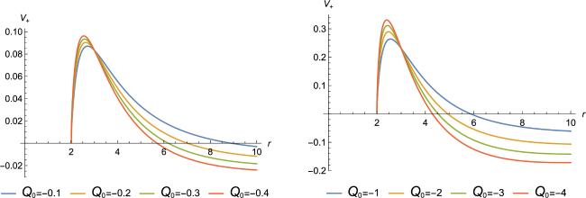
Figure 2. Variation of the potential ( |
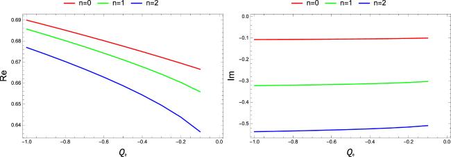
Figure 3. The QNM of a BH with M = 1. |
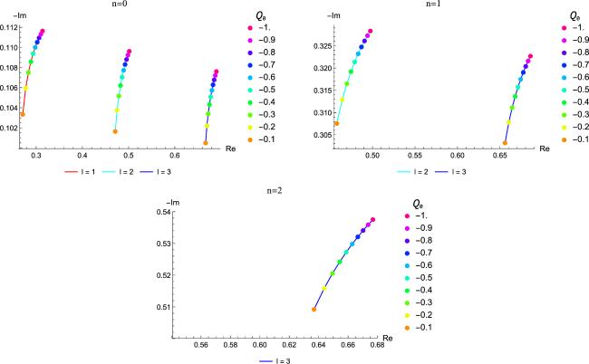
Figure 4. Complex frequency plane for l = 1, l = 2 and l = 3, showing the behavior of the quasinormal frequencies in table 1. |
Table 1. The QNM of a BH with M = 1. |
| Q0 | n | l = 1 | l = 2 | l = 3 |
|---|---|---|---|---|
| −0.1 | $\begin{array}{l}0\\ 1\\ 2\end{array}$ | $\begin{array}{l}0.270934-0.103337i\end{array}$ | $\begin{array}{l}0.471115-0.101636i\\ 0.457984-0.307536i\end{array}$ | $\begin{array}{l}0.666599-0.100494i\\ 0.655877-0.303166i\\ 0.636862-0.509225i\end{array}$ |
| −0.2 | $\begin{array}{l}0\\ 1\\ 2\end{array}$ | $\begin{array}{l}0.277386-0.105941i\end{array}$ | $\begin{array}{l}0.475056-0.103754i\\ 0.464455-0.312882i\end{array}$ | $\begin{array}{l}0.669464-0.102204i\\ 0.660328-0.307832i\\ 0.643805-0.515889i\end{array}$ |
| −0.3 | $\begin{array}{l}0\\ 1\\ 2\end{array}$ | $\begin{array}{l}0.283195-0.107492i\end{array}$ | $\begin{array}{l}0.478814-0.10516i\\ 0.469871-0.31647i\end{array}$ | $\begin{array}{l}0.672249-0.103396i\\ 0.664217-0.311084i\\ 0.649423-0.520552i\end{array}$ |
| −0.4 | $\begin{array}{l}0\\ 1\\ 2\end{array}$ | $\begin{array}{l}0.288498-0.108565i\end{array}$ | $\begin{array}{l}0.482409-0.106209i\\ 0.474687-0.319185i\end{array}$ | $\begin{array}{l}0.67496-0.104323i\\ 0.667781-0.313618i\\ 0.654326-0.524206i\end{array}$ |
| −0.5 | $\begin{array}{l}0\\ 1\\ 2\end{array}$ | $\begin{array}{l}0.293395-0.109369i\end{array}$ | $\begin{array}{l}0.485859-0.107041i\\ 0.47909-0.321365i\end{array}$ | $\begin{array}{l}0.677602-0.105082i\\ 0.671116-0.3157i\\ 0.658756-0.527231i\end{array}$ |
| −0.6 | $\begin{array}{l}0\\ 1\\ 2\end{array}$ | $\begin{array}{l}0.297954-0.110001i\end{array}$ | $\begin{array}{l}0.489179-0.107725i\\ 0.483182-0.32318i\end{array}$ | $\begin{array}{l}0.68018-0.105725i\\ 0.674276-0.317469i\\ 0.662841-0.529818i\end{array}$ |
| −0.7 | $\begin{array}{l}0\\ 1\\ 2\end{array}$ | $\begin{array}{l}0.30223-0.110515i\end{array}$ | $\begin{array}{l}0.492384-0.108302i\\ 0.487027-0.324728i\end{array}$ | $\begin{array}{l}0.682701-0.106282i\\ 0.677294-0.319005i\\ 0.666657-0.53208i\end{array}$ |
| −0.8 | $\begin{array}{l}0\\ 1\\ 2\end{array}$ | $\begin{array}{l}0.306261-0.110945i\end{array}$ | $\begin{array}{l}0.495482-0.108797i\\ 0.490668-0.326072i\end{array}$ | $\begin{array}{l}0.685166-0.106771i\\ 0.680193-0.32036i\\ 0.670256-0.53409i\end{array}$ |
| −0.9 | $\begin{array}{l}0\\ 1\\ 2\end{array}$ | $\begin{array}{l}0.310081-0.111312i\end{array}$ | $\begin{array}{l}0.498485-0.109229i\\ 0.494136-0.327255i\end{array}$ | $\begin{array}{l}0.687581-0.107206i\\ 0.682989-0.321571i\\ 0.673674-0.535897i\end{array}$ |
| −1 | $\begin{array}{l}0\\ 1\\ 2\end{array}$ | $\begin{array}{l}0.313714-0.111629i\end{array}$ | $\begin{array}{l}0.501398-0.10961i\\ 0.497454-0.328308i\end{array}$ | $\begin{array}{l}0.689948-0.107597i\\ 0.685695-0.322663i\\ 0.676937-0.537537i\end{array}$ |
5. Ringdown waveform
In this section we study the effect of the nonmetricity scalar on the ringdown waveform of a massless Dirac field. To this end, we employ the time domain integration method elaborated in [84]. The initial conditions used here are
$\begin{eqnarray}{U}_{+}({r}_{* },t)=\exp \left[-\displaystyle \frac{{\left({r}_{* }-{\hat{r}}_{* }\right)}^{2}}{2{\sigma }^{2}}\right]\quad \mathrm{and}\quad {U}_{+}({r}_{* },t){| }_{t\lt 0}=0,\end{eqnarray}$
where $\hat{r}$ and 2σ2 are taken to be 0.4 and 25, respectively. The values of Δt and Δr* are taken in order to satisfy the von Neumann stability condition, $\tfrac{{\rm{\Delta }}t}{{\rm{\Delta }}{r}_{* }}\lt 1$.In the left panel of figure 5, we provide the ringdown waveform for various values of the parameter Q0 keeping ℓ = 1, and in the right panel the waveform for various values of ℓ keeping Q0 = −0.02. From figure 5 we observe that the frequency of QNMs increases as we increase the multipole number or decrease the nonmetricity parameter. On the other hand, we can clearly conclude from the figure that the decay rate decreases with ℓ but increases with a decrease in Q0. These conclusions are in agreement with those drawn from table 1. Our study conclusively shows the significant impact that the nonmetricity parameter has on QNMs and time profile evolution of a massless Dirac field.

Figure 5. Time domain profile for a massless Dirac field. The left diagram is for various values of nonmetricity parameter Q0 with ℓ = 1 and the right one is for different multipole numbers with Q0 = −0.02. |
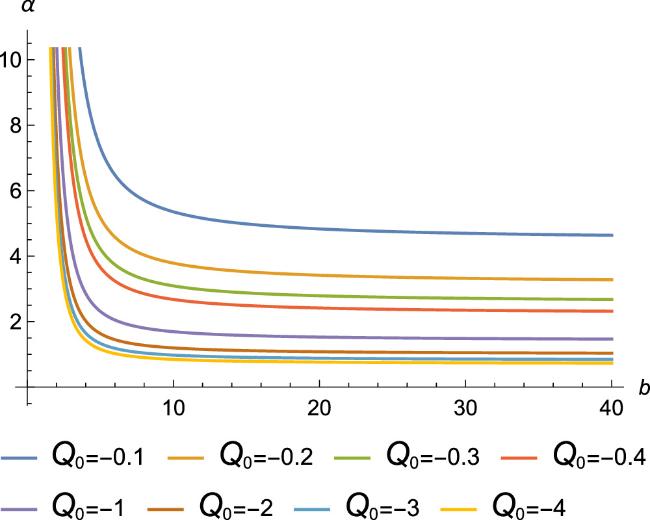
Figure 6. The behavior of deflection angle α in equation ( |
6. Deflection angle of black hole in nonplasma medium
To calculate the deflection angle α we first assume a static, spherically symmetric space–time32 ); therefore the deflection angle becomes36 ) becomes40 ) is, however, coordinate-dependent for the reason that it refers to the distance of closest approach. By using equation (38 ), we can then write40 ) in terms of M/b as follows:42 ) for different values of Q0. Figure 6 shows that the deflection angle decreases with impact parameter for all values of Q0 and remains positive.
$\begin{eqnarray}{\rm{d}}{s}^{2}=A(r){\rm{d}}{t}^{2}-B\left(r\right){\rm{d}}{r}^{2}-C\left(r\right)\left({\rm{d}}{\theta }^{2}+{\sin }^{2}\theta {\rm{d}}{\phi }^{2}\right).\end{eqnarray}$
The deflection angle α is given by [85, 86] $\begin{eqnarray}\alpha \left({r}_{0}\right)=2{\int }_{{r}_{0}}^{\infty }\displaystyle \frac{1}{C}\sqrt{\displaystyle \frac{{AB}}{\tfrac{1}{{b}^{2}}-\tfrac{A}{C}}}{\rm{d}}{r}-\pi ,\end{eqnarray}$
where r0 is the distance of closest approach of the light ray to the lens and b is the impact parameter given by $\begin{eqnarray}b=\sqrt{\displaystyle \frac{C\left(r\right)}{A\left(r\right)}}.\end{eqnarray}$
For some simple cases, the above integral can only be solved analytically. As a result, Keeton and Petters [87] proposed that this result can be approximated by a series of the form $\begin{eqnarray}\alpha \left(b\right)={a}_{0}+{a}_{1}\left(\displaystyle \frac{M}{b}\right)+{a}_{2}{\left(\displaystyle \frac{M}{b}\right)}^{2}+{a}_{3}{\left(\displaystyle \frac{M}{b}\right)}^{3}+O{\left(\displaystyle \frac{M}{b}\right)}^{4},\end{eqnarray}$
where ai are coefficients to be found. To apply this method, let us substitute the functions $\begin{eqnarray}A(r)=1-\displaystyle \frac{2M}{r},B(r)=\displaystyle \frac{-2}{{Q}_{0}{r}^{2}}{\left(1-\displaystyle \frac{2M}{r}\right)}^{-1},C\left(r\right)={r}^{2},\end{eqnarray}$
in equation ( $\begin{eqnarray}\alpha \left({r}_{0}\right)=2{\int }_{{r}_{0}}^{\infty }\displaystyle \frac{\sqrt{2}}{{r}^{2}}\sqrt{\displaystyle \frac{-{b}^{2}r}{{Q}_{0}\left({r}^{3}+{b}^{2}\left(2M-r\right)\right)}}{\rm{d}}r-\pi .\end{eqnarray}$
Let us assume the following coordinate transformation: $\begin{eqnarray}x=\displaystyle \frac{{r}_{0}}{r},h=\displaystyle \frac{M}{{r}_{0}}.\end{eqnarray}$
Then, the impact parameter becomes $\begin{eqnarray}b=\displaystyle \frac{{r}_{0}}{\sqrt{1-2\tfrac{M}{{r}_{0}}}}.\end{eqnarray}$
Therefore, equation ( $\begin{eqnarray}\alpha \left({r}_{0}\right)=2\sqrt{2}{\int }_{0}^{1}\sqrt{-\displaystyle \frac{{x}^{2}}{{Q}_{0}\left({x}^{2}-1-2h\left({x}^{3}-1\right)\right)}}{\rm{d}}{x}-\pi .\end{eqnarray}$
Assuming the weak field regime $\left(h\ll 1\right),$ then the integrand is now expanded into a Taylor series and the integral is solved term by term, giving us $\begin{eqnarray}\begin{array}{l}\alpha \left({r}_{0}\right)=-\displaystyle \frac{2\sqrt{2}}{\sqrt{-{Q}_{0}}}+\displaystyle \frac{2\sqrt{2}}{\sqrt{-{Q}_{0}}}h-\displaystyle \frac{3\sqrt{2}\left(\pi -5\right)}{\sqrt{-{Q}_{0}}}{h}^{2}\\ \,+\,\displaystyle \frac{7\sqrt{2}\left(45\pi -112\right)}{16\sqrt{-{Q}_{0}}}{h}^{3}+O{\left(h\right)}^{4}.\end{array}\end{eqnarray}$
This expression equation ( $\begin{eqnarray}\begin{array}{l}{r}_{0}=4\displaystyle \frac{M}{b}+\displaystyle \frac{15\pi }{4}{\left(\displaystyle \frac{M}{b}\right)}^{2}+\displaystyle \frac{128}{3}{\left(\displaystyle \frac{M}{b}\right)}^{3}+\displaystyle \frac{3465\pi }{64}{\left(\displaystyle \frac{M}{b}\right)}^{4}\\ \,+\,O{\left(h\right)}^{5}.\end{array}\end{eqnarray}$
Finally, we can write the deflection angle equation ( $\begin{eqnarray}\begin{array}{l}\alpha \left(b\right)=\displaystyle \frac{\sqrt{2}}{\sqrt{-{Q}_{0}}}+\displaystyle \frac{-4+3\pi }{2\sqrt{2}\sqrt{-{Q}_{0}}}\left(\displaystyle \frac{M}{b}\right)+\displaystyle \frac{26-3\pi }{2\sqrt{2}\sqrt{-{Q}_{0}}}{\left(\displaystyle \frac{M}{b}\right)}^{2}\\ \,+\,\displaystyle \frac{-384+279\pi }{16\sqrt{2}\sqrt{-{Q}_{0}}}{\left(\displaystyle \frac{M}{b}\right)}^{3}+O{\left(\displaystyle \frac{M}{b}\right)}^{4}.\end{array}\end{eqnarray}$
It is obvious that the nonmetricity scalar constant Q0 decreases the deflection angle. In order to discuss the effect of impact parameter (b) on deflection angle, we plot equation (7. Conclusion
In this work, we have considered a static and spherical BH in f(Q) gravity. f(Q) gravity is an extension of symmetric teleparallel general relativity where both curvature and torsion vanish and gravity is explained by nonmetric terms We have studied the QNMs of a massless Dirac field. We used the sixth-order WKB method to perform our calculations. We have determined how the nonmetricity parameter influences the potential and the real and imaginary parts of quasinormal frequencies. We found that as Q0 increases potential decreases. Moreover, the nonmetricity parameter has a greater influence on QNMs for real QNM values than for imaginary values, as shown in figure 3. According to figure 4, an increase in Q0 leads to a decrease in the real component and a decrease in the imaginary component. As a result of the analysis of the real and imaginary parts of the QNM frequencies, it is evident that the oscillatory frequency of the mode decreases as Q0 increases, while the damping rate increases modestly with Q0. The results obtained from the time domain analysis are in agreement with those obtained from the numerical analysis. It is necessary to understand the theory of f(Q) by studying QNMs from BHs as one of the interesting and widely studied properties of a perturbed BH space–time. In our study we demonstrate that the BH solution studied can generate significantly different QNMs from a Schwarzschild BH [88]. Furthermore, Zhao et al [89] investigated the QNMs of a test massless scalar field around static black hole solutions in f(T) gravity. We investigated how the f(T) model parameter α and orbital angular momentum l affect field decay behavior and discovered that when l increases, the period of quasinormal vibration decreases, mimicking the Schwarzschild scenario. Furthermore, the field decay behavior varies smoothly for varying α. Interestingly, our findings are identical to those in f(T) gravity.
In addition, we calculated the deflection angle using the Keeton and Petters method, which is an approximation of gravitational lensing. We discovered post-Newtonian metric coefficients by comparing the expanded metric function with the standard post-Newtonian metric. Later, we determined the bending angle coefficients and compared them with the general form of the Schwarzschild metric to obtain the final results shown in equation (42 ). Moreover, Chen et al and Wang et al [90, 91] derived a tight constraint upon the parameter space of f(T) theory by virtue of galaxy–galaxy weak lensing surveys. In this work, we use galaxy–galaxy weak gravitational lensing to obtain more precise restrictions on hypothetical departures from General Relativity. Using f(T) gravitational theories to quantify the deviation, we discovered that the quadratic correction on top of General Relativity is preferred. As shown in [92], this method can be generalized to the strong gravitational lensing case around compact astronomical objects. In [92] Jiang et al explored gravitational lensing effects within the framework of f(T) gravity, focusing on the singular isothermal sphere and singular isothermal ellipsoid mass models. They showed that under f(T) gravity, for both mass models, the deflection angle is higher than in General Relativity. In our article, we have considered static and spherically symmetric BH, whereas a BH can have charge and rotation. The presence of charge and rotation will have a quantitative effect on astrophysical observations. However, the qualitative impact of the nonmetricity scalar Q0 on astrophysical observations will remain the same for fixed values of charge and rotation, as static and spherically symmetric BHs can be considered as limiting cases of a rotating, charged BH where the rotation parameter and charge are zero.
Finally, as an application of f(Q) gravity, we examined the theoretical implications for f(Q) cosmology in terms of model construction. In general, the situation Q = Q0 can play the function of the cosmological constant in Schwarzschild-like solutions, implying a cosmological model of f(Q) gravity for dark energy. Equation (12 ) illustrates one possible functional form for f(Q). By setting the coefficients, one can create customized models of f(Q) gravity. The most basic example is the polynomial of Q, which was developed and studied as a cosmological model of f(Q) gravity [93].