


1. Introduction
Black hole thermodynamics are a fascinating field that bridge the classical and quantum facets of gravity. While essentially quantum in nature, a black hole’s (BHs) thermodynamic properties, such as entropy and temperature, correspond to more regular features like surface gravity and horizon size [1–5]. In fact, Bardeen, Carter, and Hawking’s significant study made the connection between BH fluctuations and the first law of thermodynamics by taking into account the usual reaction of a BH to infalling matter [6]. The explanation of the different variables and our knowledge of BH thermodynamics have both advanced recently. By incorporating pressure under the guise of deviations in vacuum energy, the laws of thermodynamics in gravitational mechanisms have been more thoroughly understood as an extended thermodynamical law [7–12, 87–91] and a more precise description of the BH physics has made the mass apparent as its enthalpy.
These efforts to comprehend the First Law have mainly focused on BHs, such as those found in the solutions of the Kerr–Newman family. However, there are multi-BH systems with known, precise solutions that are more fascinating. This makes such geometries suitable for thermodynamic analysis. For instance, the Israel–Khan solution [13] is an asymptotically flat structure made up of two BHs that are separated from one another by a ‘strut,’ which is a conical defect with an angular excess, that corresponds to a cosmic string with negative tension. More generally, by extending a positive-tension cosmic string through spacetime, one can give up global asymptotic flatness in order to fix the unphysical negative-tension defect [14–16]. One preserves the local asymptotic flat away from the core by doing this. Further generalising, the accelerating BH contained in the C-metric [17, 18] is made up of a BH and a cosmic string that extends [19, 20] from it as it generates an accelerating force.
A non-compact acceleration horizon also develops in this situation, in addition to asymptotic flatness being lost near the string’s extension to spatial infinity. A fixed deficiency threading the horizon or an insufficient variation during the absorption [21] of a cosmic string were the main topics of early thermodynamic studies of BH conical defects [22–25]. However, it has only recently been determined what a truly changing delay would mean in terms of thermodynamics. In particular, an asymptotically local anti-de Sitter BH that is accelerating has given rise to a situation where one can maintain fantastic computation efficiency. There has also been some progress in understanding the origin of thermodynamic length. Krtous and Zelnikov [26] discovered a thermodynamic length corresponding to the strut world volume evaluated at a specific time when considering the two BHs coupled by a strut. For similarly coupled Kerr–Newman BHs, this has since been confirmed [27].
Entropy and Bekenstein’s area are associated [1, 28] with studying the thermodynamics of BH, and the thermodynamics law can be used to calculate temperature. The corrected BH thermodynamics can be used to study many significant properties of BH, such as unstable and stable forms, criticality, holographic duality and multiple critical perspectives. The quantum-corrected fluctuations in BH thermodynamics have taken on a significant role in the study of the physics of BHs. The logarithmic correction effect of thermal fluctuations for charged anti-de Sitter BH, Horava–Lifshitz BH and Kerr-AdS BH has been calculated by Pourhassan et al [29–31]. The corrected entropy corrections for spinning BHs, Reissner–Nordstrom, Kerr, charged AdS BHs and other types of BHs have been studied by Faizal and Khalil [32]. They have also examined their remnants. For the Godel BH, the logarithmic modified entropy has been examined using the Cardy formula [33, 34] as well. Consideration of Kerr–Newman-anti-de Sitter and Reissner–Nordstrom’s BHs of 1st-order modifications to temperature and entropy has been investigated to see how the modified temperature and entropy affect anti-de Sitter BH effects on thermodynamic parameters such as internal energy, enthalpy, Helmholtz energy and Gibbs free energy [35]. In modified Hayward-BHs thermodynamics [36], the impacts of thermal fluctuations have been studied. The impact of these modification terms on thermodynamic parameters such as inner energy, pressure, entropy and specific heat has been calculated [37].
The main goal of this study is to examine the effects of the Rindler parameter and the cosmological constant on the Hawking radiation. However, the BHs are surrounded by a dilaton field and the effects of the correction parameter, the Rindler parameter, and the cosmological constant may have important contributions to thermodynamics. Moreover, we investigate the significant scales that simulate the gravity of a central object, as well as a cosmic constant and Rindler parameter, which is a term that establishes the physical scales and subleading terms to the leading order in the significant radius expansion. With the exception of the Rindler term, general relativity also predicts all of these statements. Every realistic item passes through a transitional phase when it transitions from an unstable to a stable state, as indicated by Gibbs free energy and heat capacity transmission from a negative to a positive area. Heat capacity dissipation reveals the crucial points for phase transition.
We proceed with our study in this manuscript in the following scheme: in section 2 , we explain the brief review of Rindler–Schwarzschild black hole. In section 3 , we discuss the physical existence of BH by explaining the geometric mass and Hawking temperature. In section 4 , we study the corrected entropy. In section 5 , we study the thermal stability of BH by discussing the heat capacity and Gibbs free energy. Section 6 , discusses the emission energy process of BH. In the last section 7 , we write a brief summary of our concluding remarks.
2. Introductory review of the Rindler–Schwarzschild black hole
Assume a four-dimensional symmetric spherically line element defines spacetime [38] as1 ) for every line element solution. The test particles are then considered to travel in the background of a four-dimensional metric (1 ). For further information, see [39]. The technique of spherical reduction [40] can reduce the four-dimensional Einstein–Hilbert action to a specific two-dimensional dilaton gravity model. This approach is novel in that it allows for infrared changes to the dilaton gravity model. The following assumptions are compatible with the general theory for two-dimensional geometry with field content f and Ξ. To begin, we assume that all non-renormalizable terms have been removed; therefore, the theory must be power-counting renormalizable. This precisely refers to the action [41, 42] as2 ) has to be done. In the four-dimensional structure words, we consider extensive surface regions surrounding a central item. At spherical reduction, the limit of an immense dilaton field (Ξ) follows the limit of enormous surface areas. We analyse the possibility of V performing in the following ways:3 ) for the potential V is critical to the discussion, let us take some time to explain its justification. Physics shows that the leading term Ξ in the huge expansion is quadratic, and that if we take permit powers bigger than Ξ2, the resulting spacetime has a curvature singularity for large Ξ. As a result, the equation (3 ) is the universal asymptotic result requiring the absence of curvature singularity and analytic in Ξ in the infrared domain. With the impacts of the initial three terms in (3 ), the term $O(\tfrac{1}{{\rm{\Xi }}})$ contributes to the gravitational potential in a proportionate way to $\mathrm{ln}r/r$. In the extreme infrared region, these effects are subordinate. As a result, we reject this sentence (along with other subleading phrases). We can fix the subleading coefficients in the asymptotic potential (3 ) by immediately re-scaling Ξ and k, which refers to setting up the physical length scale. We used b = 2 to preserve universality. The action (2 ) is reduced to eliminating all asymptotically subleading terms and selecting adequate normalisation of the coupling constants k = 1 as4 ) provides a theory whose existence depends upon the coupling constant a. The descending EOM solutions (4 ) are identified as a spherically symmetric solution (1 ) that model gravity in the infrared domain. It is easy to find solutions for the EOM [43] given as:8 ), M is an integral constant related to the mass (AdM mass) of the Rindler–Schwarzschild black hole [45], and a is Rindler coupling parameter [43]. It is obvious that the considered spacetime transforms [45] into the well-known Schwarzschild BH for a = 0 = Λ. This study examines the geodesic evaluation of Grumiller’s metric, which measures gravity over extended distances. The Rindler parameter can be compared to the Schwarzschild geodesic [47]. Furthermore, the Rindler–Schwarzschild black hole temperature was compared to the Schwarzschild BH in [48]. The black hole possesses Rindler parameter; hence, it is also known as the Rindler-improved Schwarzschild BH [49].
$\begin{eqnarray}{{\rm{d}}{s}}^{2}={f}_{\mu \nu }{{\rm{d}}{x}}^{\mu }{{\rm{d}}{x}}^{\nu }+{{\rm{\Xi }}}^{2}\left({\sin }^{2}\theta {\rm{d}}{\phi }^{2}+{\rm{d}}{\theta }^{2}\right).\end{eqnarray}$
In classical dynamics, the two-dimensional theory of equations of motion (EOM) leads to a four-dimensional metric ( $\begin{eqnarray}S=-\displaystyle \frac{1}{{k}^{2}}\int {{\rm{d}}}^{2}x\sqrt{-{\boldsymbol{f}}}\left[f({\rm{\Xi }})R+2{\left(\partial {\rm{\Xi }}\right)}^{2}-2V({\rm{\Xi }})\right].\end{eqnarray}$
Consider an appropriate form for the kinetic term associated with the dilaton field Ξ via field redefinition. This assumption is not substantially dependent on the gravitational coupling constant (k). We assume that the free functions f and V are analytic in Ξ for large d, as in spherically omitted GR [39]. According to the EOM analysis, in order to reproduce the Newton potential ($-\tfrac{M}{r}$), the coupling function f that multiplies the Ricci scalar R must be supplied by f = Ξ2 [43]. When f = cΞ2 is taken into account, the potential changes to $-\tfrac{M}{{r}^{1/c}}$ and ∣c − 1∣ < 10−10 [44] is an observational bound for c. If the power of Ξ in the function f was modified, it would result in an exponential growth or decay of the potential. Further, we make the cautious assumption that f = cΞ2 is not renormalized in the infrared, which agrees perfectly with the experimental data. Choosing the possible V in the reaction ( $\begin{eqnarray}V({\rm{\Xi }})={\rm{\Lambda }}{{\rm{\Xi }}}^{2}+a{\rm{\Xi }}+b+O\left(\displaystyle \frac{1}{{\rm{\Xi }}}\right).\end{eqnarray}$
Because the ansatz ( $\begin{eqnarray}S=-\int {{\rm{d}}}^{2}x\sqrt{-{\boldsymbol{f}}}\left[{{\rm{\Xi }}}^{2}R+2{\left(\partial {\rm{\Xi }}\right)}^{2}+8a{\rm{\Xi }}-6{\rm{\Lambda }}{{\rm{\Xi }}}^{2}+2\right].\end{eqnarray}$
It provides a generic, efficient theory of relativity in the infrared region that is consistent with the preceding conditions. The action ( $\begin{eqnarray}R=\displaystyle \frac{2}{{\rm{\Xi }}}{f}^{\mu \nu }{{\rm{\Delta }}}_{\mu }{\partial }_{\nu }{\rm{\Xi }}-\displaystyle \frac{4a}{{\rm{\Xi }}}-6{\rm{\Lambda }},\end{eqnarray}$
$\begin{eqnarray}{f}_{\alpha \beta }V({\rm{\Xi }})=2{\rm{\Xi }}({{\rm{\Delta }}}_{\alpha }{\partial }_{\beta }-{f}_{\alpha \beta }{{\rm{\Delta }}}^{\mu }{\partial }_{\mu }){\rm{\Xi }}-{f}_{\alpha \beta }{\left(\partial {\rm{\Xi }}\right)}^{2}.\end{eqnarray}$
In [45–46], a spherically symmetric four-dimensional line element can be obtained as $\begin{eqnarray}{{\rm{d}}{s}}^{2}=f(r){{\rm{d}}{t}}^{2}-\displaystyle \frac{{{\rm{d}}{r}}^{2}}{f(r)}-{r}^{2}\left({\sin }^{2}\theta {\rm{d}}{\phi }^{2}+{\rm{d}}{\theta }^{2}\right),\end{eqnarray}$
with $\begin{eqnarray}f(r)=2{ar}-\displaystyle \frac{2M}{r}-{\rm{\Lambda }}{r}^{2}+1\,\,{and}\,\,{\rm{\Xi }}={r}^{2}.\end{eqnarray}$
In equation (Here we choose Λ = –8πP [50]. Here, pressure P is directly linked with the cosmological constant Λ, thus by taking the negative value of pressure we consider the anti-de Sitter spacetime (AdS-spacetime), and for positive values of P, we mean de Sitter spacetime (dS-spacetime) [51]. In this manuscript we analyze the black hole thermodynamics for both AdS-spacetime and dS-spacetime. The possible existence of positive and negative event horizons can be predicted by the physical behavior of lapse function f(r) as shown in figure 1. It is obvious that for the fixed value of Rindler parameter a, positive pressure P depicts the positive event horizon and negative pressure P shows the negative event horizon along radial coordinate. For fixed positive pressure P, increasing values of a depict the increasing possibility of positive event horizon.
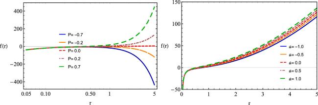
Figure 1. The figure shows the lapse function, f(r), plotted against radius, r. Fixed parameters are M = 1, P = 0.2, a = 0.5. |
3. Physical existence of the Rindler–Schwarzschild black hole
The utilization of the lapse function provided by equation (8 ) to determine the mass of the BH confers significant importance. It signifies the presence of the BH in a physical sense. It is important to know that positive mass indicates stable BH, whereas negative mass indicates towards the instability of the BH. There are several approaches to calculating the mass of a black hole like the conformal approach [52–54], by using the first law of thermodynamics [55, 56]. Here, we calculate the geometric mass by setting f(r) = 0 [57, 58]. The ensuing equation furnishes the geometric mass of the BH, specifically in the context of our BH solution it is given as:
$\begin{eqnarray}M=\displaystyle \frac{1}{2}{r}_{0}\left(2{{ar}}_{0}+8\pi {{\Pr }}_{0}^{2}+1\right),\end{eqnarray}$
where r0 is the BH horizon radius. We plot the geometric mass of the BH along horizon radius r0 in figure 2. It is obvious that for the fixed value of Rindler parameter a, positive pressure P depicts the positive mass, and negative pressure P shows the negative mass along event horizon r0. For fixed positive pressure P, increasing values of a depicted mass is positive. Thus pressure P and all values of a depict the stability of our solution of the Rindler–Schwarzschild BH.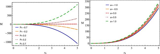
Figure 2. Geometric mass M and values of fixed parameters are P = 0.2, a = 0.5. |
The Hawking temperature TH of the BH can be determined [59, 60] by $\tfrac{{f}^{{\prime} }(r)}{4\pi }$ as:
$\begin{eqnarray}{T}_{H}=\displaystyle \frac{a+\tfrac{M}{{r}_{0}^{2}}+8\pi {{\Pr }}_{0}}{2\pi }.\end{eqnarray}$
The entropy of the BH can be written as [28]: $\begin{eqnarray}S=\pi {r}_{0}^{2}\end{eqnarray}$
4. Corrected entropy
In this section, we investigate the impact of thermal fluctuations on the thermodynamics of the Rindler–Schwarzschild BH. To study this phenomenon, we utilize the formalism of Euclidean quantum gravity, which involves rotating the temporal coordinate within a complex plane. As a result, the partition function for the BH can mathematically be found in the references [61–66]. Specifically detailed calculations can be found in reference [62], where the simplified action is given as:10 ) and (21 ), we can obtain the following expression for the corrected entropy
$\begin{eqnarray}Z=\int {DgDA}\exp (-I),\end{eqnarray}$
where $I\to \iota \hat{I}$ is the Euclidean action of the field for this system, and the integral is taken over all fields that justify some periodicity or boundary condition. One can relate the statistical mechanical partition function [67, 68] as $\begin{eqnarray}Z={\int }_{0}^{\infty }{DE}{\rm{\Gamma }}(E)\exp (-\psi E),\end{eqnarray}$
where ψ = T−1. We can calculate the density of states by using $\begin{eqnarray}{\rm{\Gamma }}(E)=\displaystyle \frac{1}{2\pi i}{\int }_{{\psi }_{0}-{\rm{i}}\infty }^{{\psi }_{0}+{\rm{i}}\infty }{\rm{d}}\psi {{\rm{e}}}^{S(\psi )},\end{eqnarray}$
where ${S}_{c}=\psi E+\mathrm{ln}Z$. The entropy near the equilibrium temperature ψ can be calculated by neglecting thermal fluctuations, which yields $S=\pi {r}_{0}^{2}$. But, when we are taking into account thermal fluctuations then the entropy Sc(ψ) is given by [61]: $\begin{eqnarray}{S}_{c}=S+\displaystyle \frac{1}{2}\left(\psi -{\psi }_{0}\right){\left(\displaystyle \frac{{\partial }^{2}S(\psi )}{\partial {\psi }^{2}}\right)}_{\psi ={\psi }_{0}}.\end{eqnarray}$
So, one can write the density as stated by: $\begin{eqnarray}{\rm{\Gamma }}(E)=\displaystyle \frac{1}{2\pi i}{\int }_{{\psi }_{0}-{\rm{i}}\infty }^{{\psi }_{0}+{\rm{i}}\infty }{\rm{d}}\psi {{\rm{e}}}^{\tfrac{1}{2}\left(\psi -{\psi }_{0}\right){\left(\tfrac{{\partial }^{2}S(\psi )}{\partial {\psi }^{2}}\right)}_{\psi ={\psi }_{0}},}\end{eqnarray}$
which leads to $\begin{eqnarray}{\rm{\Gamma }}(E)=\displaystyle \frac{{{\rm{e}}}^{S}}{\sqrt{2\pi }}{\left[{\left(\displaystyle \frac{\left.{{\rm{\partial }}}^{2}S(\psi \right)}{{\rm{\partial }}{\psi }^{2}}\right)}_{\psi ={\psi }_{0}}\right]}^{\tfrac{1}{2}}.\end{eqnarray}$
We can write corrected entropy as $\begin{eqnarray}{S}_{c}=S-\displaystyle \frac{1}{2}\mathrm{ln}{\left[{\left(\displaystyle \frac{{\partial }^{2}S(\psi )}{\partial {\psi }^{2}}\right)}_{\psi ={\psi }_{0}}\right]}^{\tfrac{1}{2}}.\end{eqnarray}$
The second derivative of entropy provides a measure of the squared fluctuation of energy. By utilizing the connection between conformal field theory and the microscopic degrees of freedom of a BH [69], it becomes possible to simplify this expression. Consequently, the entropy can be expressed as $S={m}_{1}{\psi }^{{n}_{1}}+{m}_{2}{\psi }^{-{n}_{2}}$, where m1, m2, n1, and n2 are positive constants [34]. This entropy exhibits an extremum at ${\psi }_{0}={\left(\tfrac{{{mn}}_{2}}{{m}_{1}{n}_{1}}\right)}^{\tfrac{1}{{n}_{1}+{n}_{2}}}={T}_{H}^{-1}$, where TH denotes hawking temperature. By expanding the entropy around this extremum, we can determine [70, 71]: $\begin{eqnarray}{\left(\displaystyle \frac{{\partial }^{2}S(\psi )}{\partial {\psi }^{2}}\right)}_{\psi ={\psi }_{0}}=S{\psi }_{0}^{-2}.\end{eqnarray}$
A corrected version of entropy by negating higher-order correction terms can be written as $\begin{eqnarray}{S}_{c}=S-\displaystyle \frac{1}{2}\,{\rm{ln}}{\,{ST}}_{H}^{2}.\end{eqnarray}$
Furthermore, the presence of quantum fluctuations in the geometry of BHs introduces a notable concern regarding thermal fluctuations in BH thermodynamics. These correction terms become significant when the size of the BH is small and its temperature is large. Hence, for large BHs, quantum fluctuations can be disregarded. It becomes evident that thermal fluctuations become significant solely for BHs characterized by high temperatures, and as the BH size decreases, its temperature increases. Thus, we can deduce that these correction terms are applicable solely to sufficiently small BHs exhibiting high temperatures [61]. Subsequently, we can derive the general expression for entropy by neglecting higher-order correction terms $\begin{eqnarray}{S}_{c}=S-\gamma \mathrm{ln}{{ST}}_{H}^{2}.\end{eqnarray}$
Here, we introduce γ as a constant parameter to incorporate the logarithmic correction terms associated with thermal fluctuations. By setting γ = 0, we recover the entropy without any correction terms As mentioned earlier, in the case of large BHs with extremely low temperatures, we can take γ → 0, whereas, for small BHs with sufficiently high temperatures, we consider γ → 1. By utilizing equations ( $\begin{eqnarray}{S}_{c}=\pi {r}_{0}^{2}-\gamma \mathrm{log}\left(\displaystyle \frac{{r}_{0}^{2}{\left(4a+\tfrac{24\pi {{\Pr }}_{0}^{2}+1}{\sqrt{{r}_{0}^{2}}}\right)}^{2}}{16\pi }\right).\end{eqnarray}$
We plot SC considering different choices of the correction parameter: γ = 0 for large black holes, γ = 0.2, 0.5, 0.8 & 1.0 for small black holes (0 < γ < 1), and γ = 1 for smaller black holes. The plot shown in figure 3 demonstrates that the entropy of spacetime consistently increases across the entire range considered for different values of γ with both positive and negative fixed values of pressure P. Moreover, for positive pressure, there is no fluctuation, while fluctuation can be observed for negative pressure. Notably, these fluctuations are more pronounced for smaller black holes. One can also observe an initial decrease in corrected entropy for different values of P & a by attaining the negative value, after that it increases continuously by maintaining the positive value. In the coming discussions, we calculate the other thermodynamic properties of BHs using this corrected entropy and compare the results by setting γ = 0 for no correction and γ = 1 for correction terms. Now, we determine the thermodynamic temperature T by using the first law of thermodynamics [55, 72]: $\begin{eqnarray}{\rm{d}}{M}={T}{\rm{d}}{S},\end{eqnarray}$
which yields the temperature as written below $\begin{eqnarray}T=\displaystyle \frac{-24\gamma \,P\,{\rm{log}}\left(\tfrac{{\left(4a\sqrt{{r}_{0}^{2}}+24\pi {Pr}_{0}^{2}+1\right)}^{2}}{16\pi }\right)+24\pi {Pr}_{0}^{2}+1}{4\sqrt{\pi }\sqrt{\pi {r}_{0}^{2}-\gamma {\rm{log}}\left(\tfrac{{\left(4a\sqrt{{r}_{0}^{2}}+24\pi {Pr}_{0}^{2}+1\right)}^{2}}{16\pi }\right)}}+\displaystyle \frac{a}{\pi }.\end{eqnarray}$
For the next calculations, we incorporate the above calculated thermodynamic temperature T. We plot the temperature T in figure 4. One can see that in large BHs (γ = 0), for the fixed value of a and variable P, the BH is initially stable for small event horizon r0 and afterward, for positive pressure the BH is globally unstable, whereas for negative pressure the BH is globally stable. For fixed pressure P and varying values of a. In small BHs (γ = 1), for the fixed value of a and variable P, the BH is unstable (T < 0) for positive pressure and the BH is stable (T > 0) for negative pressure. For the fixed values of P, the BH is stable (T > 0) in the case of both positive and negative a.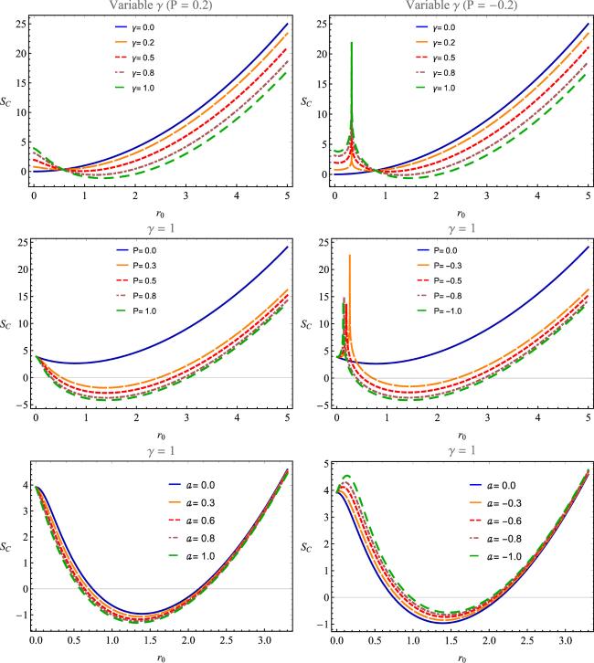
Figure 3. Corrected entropy SC. Values of fixed parameters are P = 0.2, a = 0.5. |

Figure 4. The figure shows temperature T versus the black hole horizon radius r0. Fixed parameters are P = 0.2, a = 0.5. |
5. Thermal stability and phase transition
The thermal stability of the BH is examined by studying the behavior of the heat capacity CP over both positive and negative intervals. Positive values of CP signify the existence of a stable region, whereas negative values indicate an unstable region. Furthermore, the heat capacity plays a crucial role in interpreting phase transitions through its divergence [73–77]. In the case of the Rindler–Schwarzschild BH, the expression for the heat capacity can be represented as follows
$\begin{eqnarray}\begin{array}{rcl}{C}_{P} & = & \displaystyle \frac{2\left(-4a\gamma \sqrt{{r}_{0}^{2}}+4\pi a{\left({r}_{0}^{2}\right)}^{3/2}+24{\pi }^{2}{{\Pr }}_{0}^{4}+\pi {r}_{0}^{2}(1-48\gamma P)\right)}{{C}_{1}}\\ & & \times \,\left[\pi {r}_{0}^{2}-\gamma \mathrm{log}\left[\displaystyle \frac{{\left(4a\sqrt{{r}_{0}^{2}}+24\pi {{\Pr }}_{0}^{2}+1\right)}^{2}}{16\pi }\right]\right]\\ & & \times \,\left[-24\sqrt{\pi }\gamma P\mathrm{log}\left[\displaystyle \frac{{\left(4a\sqrt{{r}_{0}^{2}}+24\pi {{\Pr }}_{0}^{2}+1\right)}^{2}}{16\pi }\right]\right.\\ & & +4a\sqrt{\pi {r}_{0}^{2}-\gamma \mathrm{log}\left[\displaystyle \frac{{\left(4a\sqrt{{r}_{0}^{2}}+24\pi {{\Pr }}_{0}^{2}+1\right)}^{2}}{16\pi }\right]}\\ & & \left.+24{\pi }^{3/2}{{\Pr }}_{0}^{2}+\sqrt{\pi }\Space{0ex}{4.45ex}{0ex}\right],\end{array}\end{eqnarray}$
where $\begin{eqnarray*}\begin{array}{c}\begin{array}{rcl}{C}_{1} & = & \sqrt{\pi }\sqrt{{r}_{0}^{2}}\left(4a\left(\pi {r}_{0}^{2}-\gamma \right)+\pi \sqrt{{r}_{0}^{2}}\left(24P\left(\pi {r}_{0}^{2}-2\gamma \right)+1\right)\right)\\ & & \times \,\left[-24\gamma P{\rm{log}}\left[\displaystyle \frac{{\left(4a\sqrt{{r}_{0}^{2}}+24\pi {{\Pr }}_{0}^{2}+1\right)}^{2}}{16\pi }\right]\right.\\ & & \left.+\,24\pi {{\Pr }}_{0}^{2}-1\Space{0ex}{4.27ex}{0ex}\right]\end{array}\end{array}.\end{eqnarray*}$
Figure 5 shows the heat capacity in small and large BHs. It can be identified that for large BHs (γ = 0) in the case of variable pressure P, BHs shift the transition originally from unstable (CP < 0) to the globally stable region (CP > 0) for both positive and negative pressure, whereas for P = 0 it shows the global instability (CP < 0). Also for variable a, BHs shift the transition from unstable (CP < 0 near event horizon r0) to the stable region (CP > 0) for all values of a. In the case of smaller BHs (γ = 1), the BHs show global stability (CP > 0) for small positive and negative values of P (i.e., P = 0.2, –0.2), whereas for large positive and negative values of pressure P (P = 0.7, –0.7), BHs are initially stable (CP > 0) then transit into the unstable region (CP < 0) and enter the globally stable region (CP > 0). And fixed pressure BHs are globally stable (CP > 0) for all values of a. If we talk about the phase transition points related to heat capacity for fix a = 0.5 & γ = 0: we observe singularity between r0 = (0.142, 0.173) for P = –0.7, and r0 = (0.317, 0.348) for P = − 0.2, there is no phase transition for p = 0. For P = 0.2, the phase transition point lies between r0 = (0.242, 0.274), and for P = 0.7 the phase transition point lies between (r0 = 0.122, 0.154). By fixing a = 0.5 γ = 1, we get the following information: we observe singularity between r0 = (0.003, 0.0345) for P = –0.7, and r0 = (0.044, 0.076) for P = –0.2. There is no phase transition for p = 0, and for P = 0.2, the phase transition point lies between r0 = (0.713, 0.745), and for P = 0.7 phase transition point lies between r0 = (0.35, 1.30). Then, by fixing P = 0.2 γ = 0, we obtain the following information: the phase transition point for a = − 1 is r0 = 0.25. For a = − 0.5, the phase transition point is r0 = 0.2575. For a = 0.0, the phase transition point is r0 = 0.257 52. For a = 0.5, the phase transition point is r0 = 0.257 516 2. For a = 1.0, the phase transition point is r0 = 0.2576. For fixing P = 0.2 γ = 1, for all the selected values of a, CP > 0, thus shows no phase transition.
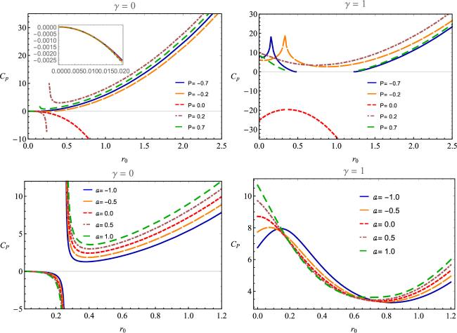
Figure 5. Heat capacity CP. Values of fixed parameters are P = 0.2, a = 0.5. |
Figure 6 gives us information regarding the phase transition between large and small BHs. For γ = 0 (Large BH), the temperature is low and for γ = 1 (small BH), the temperature is high. Thus for negative pressure (P = –0.7), the critical point is r0 = 0.4 where it shifts the transition between small and large BH. For positive pressure (P = 0.7), the critical point is r0 = 0.325 & 0.350, where it shifts the transition between small and large BHs.

Figure 6. Heat capacity CP for fixed constant a = 0.5. |
Apart from heat capacity, the analysis of BH phase transitions also relies on the examination of Gibbs free energy. The Gibbs free energy exhibits unique features, including a ‘swallowing tail’, which assists in identifying the first-order phase transition point characterized by a discontinuity in its first-order derivative. Additionally, the continuous but non-smooth behavior of both the Gibbs free energy and its first-order derivative can indicate a second-order phase transition [78]. The computation of the Gibbs free energy can be performed using the formula [78] given as:
$\begin{eqnarray}\begin{array}{l}G=M-{TS}=\displaystyle \frac{1}{2}{r}_{0}\left(2{{ar}}_{0}+8\pi {{\Pr }}_{0}^{2}+1\right)\\ -\left[\pi {r}_{0}^{2}-\gamma \mathrm{log}\left[\displaystyle \frac{{\left(4a\sqrt{{r}_{0}^{2}}+24\pi {{\Pr }}_{0}^{2}+1\right)}^{2}}{16\pi }\right]\right]\\ \times \left[\displaystyle \frac{-24\gamma P\mathrm{log}\left(\tfrac{{\left(4a\sqrt{{r}_{0}^{2}}+24\pi {{\Pr }}_{0}^{2}+1\right)}^{2}}{16\pi }\right)+24\pi {{\Pr }}_{0}^{2}+1}{4\sqrt{\pi }\sqrt{\pi {r}_{0}^{2}-\gamma \mathrm{log}\left(\tfrac{{\left(4a\sqrt{{r}_{0}^{2}}+24\pi {{\Pr }}_{0}^{2}+1\right)}^{2}}{16\pi }\right)}}+\displaystyle \frac{a}{\pi }\right].\end{array}\end{eqnarray}$
One can get detailed information about the phase transition points in both cases of larger BHs (γ = 0) and smaller BHs (γ = 1) through the graphical behavior of Gibbs free energy in figure 7.
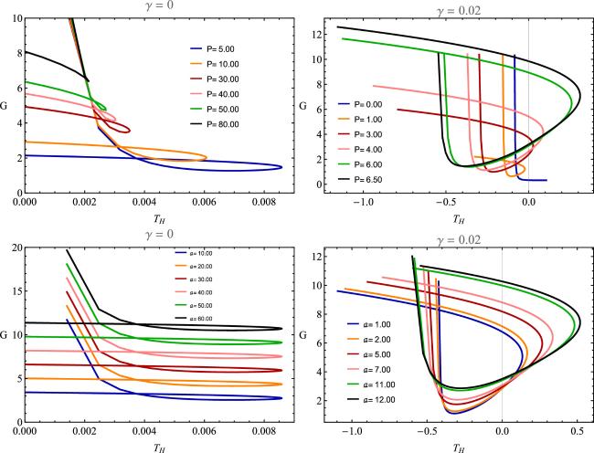
Figure 7. Gibbs free energy G. Values of fixed parameters are M = 0.002, P = 5.0, a = 2.0. |
6. Emission energy
Quantum fluctuations occurring within the interior of BHs results in the continual creation and annihilation of particles beyond the event horizon in large quantities. This tunneling phenomenon [79–83] causes positively charged particles to be attracted toward the innermost region of the BH, which leads to the emission of Hawking radiation and eventual evaporation of the BH over a specific period. The rate of evaporation is directly proportional to the energy emission rate. From the perspective of a distant observer, the high-energy reception cross-section closely approximates the BH shadow. This energy reception cross-section exhibits oscillations around a fixed, constrained value denoted as ${\sigma }_{{lim}}$, which corresponds to the radius of the BH [84–86]:24 ). One can get the expression for the emission energy process from equation (28 ) after replacing the horizon radius r0, temperature T, and cross-section ${\sigma }_{{lim}}$:
$\begin{eqnarray}{\sigma }_{{\rm{lim}}}\approx \pi {r}_{0}^{2},\end{eqnarray}$
where, r0 is the event horizon radius of BH. Thus, the expression for the energy emission rate of BH is [85, 86] $\begin{eqnarray}\displaystyle \frac{{{\rm{d}}}^{2}\varepsilon }{{\rm{d}}\omega {\rm{d}}{t}}=\displaystyle \frac{2{\pi }^{2}{\sigma }_{{\rm{lim}}}}{{{\rm{e}}}^{\tfrac{\omega }{T}}-1}{\omega }^{3},\end{eqnarray}$
where, the temperature T is given in equation ( $\begin{eqnarray}\begin{array}{l}\displaystyle \frac{{{\rm{d}}}^{2}\varepsilon }{{\rm{d}}\omega {\rm{d}}{t}}=\left(2{\pi }^{3}{r}_{0}^{2}\right){\omega }^{3}\left[\Space{0ex}{7.25ex}{0ex}\exp \left[\Space{0ex}{7.25ex}{0ex}\omega \right.\right.\\ \times \left[\Space{0ex}{7.35ex}{0ex},[,\right.\displaystyle \frac{-24\gamma P\mathrm{log}\left(\tfrac{{\left(4a\sqrt{{r}_{0}^{2}}+24\pi {{\Pr }}_{0}^{2}+1\right)}^{2}}{16\pi }\right)+24\pi {{\Pr }}_{0}^{2}+1}{4\sqrt{\pi }\sqrt{\pi {r}_{0}^{2}-\gamma \mathrm{log}\left(\tfrac{{\left(4a\sqrt{{r}_{0}^{2}}+24\pi {{\Pr }}_{0}^{2}+1\right)}^{2}}{16\pi }\right)}}\\ {\left.\left.{\left.\Space{0ex}{7.25ex}{0ex}+\,\displaystyle \frac{a}{\pi }\right]}^{-1}\right]-1\right]}^{-1}.\end{array}\end{eqnarray}$
One can obtain information about emission energy from figure 8. One can see that ϵωt increases with increasing values of P & a for both large and small BHs. Moreover ϵωt∣γ=0 > ϵωt∣γ=1.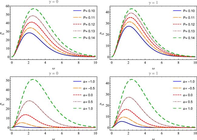
Figure 8. Emission energy ϵωt. Values of fixed parameters are P = 0.10, a = 0.5. |
7. Conclusion
In our current analysis, we delve into the study of a new type of BH solution called the Rindler–Schwarzschild BH, which is differentiated through the parameters a from the Schwarzschild BH solution. When a = 0, the solution corresponds to the original Schwarzschild BH. It is important to note that the Rindler–Schwarzschild BH is thermodynamically stable. We consider the pressure $P=-\tfrac{1}{8\pi }{\rm{\Lambda }}$. We investigate the thermal stability of the solution by analyzing its temperature and heat capacity, as well as its phase transition via heat capacity and Gibbs free energy analysis, thermal fluctuations, and mass evaporation through energy emission by comparing the small and large BHs and also the results with the Schwarzschild BH by setting a = 0.
Our study shows that the positive behavior of the metric function f(r) and mass M ensure the physical existence of Rindler–Schwarzschild BHs. The temperature T > 0 predicts the physical existence of the solutions, and CP > 0 ensures the thermally stable hairy BHs. As decay is natural in realistic objects, the evaporation of mass is predicted through the energy emission process. Every realistic object undergoes a transitional phase while turning from an unstable to a stable state, as evidenced by the swallowing behaviors of Gibbs free energy and transmission of heat capacity from negative to positive region. The critical points for phase transition are apparent in heat capacity dissipation.
In the domain of a very short event horizon, we observe the monotonically increasing behavior of entropy in the case of small BHs and negative pressure P. The height of entropy decreases for a specific value of the radii, which signifies an abrupt change and represents a thermal fluctuation in the system. We also find that small BHs (0 < γ ≤ 1) are more affected by thermal fluctuations. Whereas no fluctuation process occurs in the case of positive P and larger black holes (γ = 0). Furthermore, Rindler–Schwarzschild BHs exhibit natural evaporation. In summary, this study has physical significance in predicting the existence of realistic small and large Rindler–Schwarzschild BHs.