


1. Introduction
2. $f({\mathbb{R}},{\mathbb{T}})$ theory admitting Einstein–Maxwell field equations
3. Gravitational decoupling
4. Finch–Skea ansatz and matching criteria
5. Reviewing physical constraints admitted by compact models
| (a)Addressing the presence of a singularity within a compact structure is a fundamental concern that forms the basis of our investigation. In our quest to validate the singularity-free nature of the Finch–Skea components, we checked the following criteria. In addition, it is imperative to determine their outwardly increasing behavior. Here, we have $\begin{eqnarray*}\begin{array}{l}{{\rm{e}}}^{{b}_{1}(r)}{| }_{r=0}={c}_{1}^{2},\quad {{\rm{e}}}^{{b}_{2}(r)}{| }_{r=0}=1.\end{array}\end{eqnarray*}$ Upon computing the first derivatives of these potentials, we arrived at $\begin{eqnarray*}\begin{array}{l}({{\rm{e}}}^{{b}_{1}(r)})^{\prime} =2{c}_{2}\sqrt{{c}_{3}}r\left(\displaystyle \frac{1}{2}{c}_{2}\sqrt{{c}_{3}}{r}^{2}+{c}_{1}\right),\quad ({{\rm{e}}}^{{b}_{2}(r)})^{\prime} =2{c}_{3}r,\end{array}\end{eqnarray*}$ finding them both zero in the core. This confirms the nondecreasing behavior of metric components and thereby establishes the validity of employing the Finch–Skea ansatz. | |
| (b)Understanding the fundamental properties of matter-related factors is of paramount importance. These elements should maintain finite and positive values across the whole domain. Moreover, they should attain their maximum (minimum) values at the center (outer boundary). Similarly, it can be established that the decrement in these factors while moving outward is assured when the first derivatives of these parameters vanish at r = 0 while exhibiting a negative profile outward. Further, anisotropy also plays a crucial role in increasing or decreasing the collapse rate of a celestial body [71–73]. | |
| (c)The spherical mass function can be determined using two approaches, accounting for its geometric properties and fluid distribution. In this regard, we opted for the latter approach to calculate the corresponding mass. The mathematical representation for this is given as $\begin{eqnarray}m(r)=\displaystyle \frac{1}{2}{\int }_{0}^{R}{s}^{2}\mu {\rm{d}}{s}.\end{eqnarray}$ In the following, we used $\tilde{\mu }$ instead of μ to explore the effects of the modified theory on the mass function. Within the realm of astrophysics, the concept of compactness plays a pivotal role in characterizing the density of mass within a given region. This factor, often denoted as ν(r), is the ratio of mass to size (radius) of a compact celestial body. A high value of compactness signifies an extraordinary concentration of matter within a remarkably small volume, resulting in the propagation of powerful gravitational attraction. When a spherical body is considered, this factor must be less than $\tfrac{4}{9}$ [74]. When self-gravitating objects interact with potent gravitational effects produced by neighboring bodies, their surfaces emit light and electromagnetic radiation. Measuring the increment in their wavelength is known as redshift and can be expressed as follows: $\begin{eqnarray}z(r)={\left\{1-2\nu (r)\right\}}^{\tfrac{-1}{2}}-1{\rm{.}}\end{eqnarray}$ It should be highlighted that the maximum value of this parameter is 5.211 [75], whereas it is comparatively lower in an isotropic configuration. | |
| (d)Exploring energy conditions is indeed an important aspect when investigating compact fluid configurations. This exploration is pivotal for assessing the viability of the internal structure. The essential criterion for confirming the presence of usual matter is to have a positive profile of the matter variables throughout. If any of these conditions is not met, this suggests the existence of exotic fluids within the structure. For the anisotropic interior, they are $\begin{eqnarray}\begin{array}{l}\mu +\displaystyle \frac{{q}^{2}}{8\pi {r}^{4}}\geqslant 0,\quad \mu +{P}_{\perp }+\displaystyle \frac{{q}^{2}}{4\pi {r}^{4}}\geqslant 0,\quad \mu +{P}_{r}\geqslant 0,\\ \mu -{P}_{\perp }\geqslant 0,\quad \mu -{P}_{r}+\displaystyle \frac{{q}^{2}}{4\pi {r}^{4}}\geqslant 0,\quad \mu +2{P}_{\perp }+{P}_{r}+\displaystyle \frac{{q}^{2}}{4\pi {r}^{4}}\geqslant 0.\end{array}\end{eqnarray}$ In practice, the fulfillment of the dominant conditions, such as $\mu -{P}_{r}+\tfrac{{q}^{2}}{4\pi {r}^{4}}\geqslant 0$ and μ − P⊥ ≥ 0, is sufficient, rendering the fulfillment of all other conditions a mere formality. | |
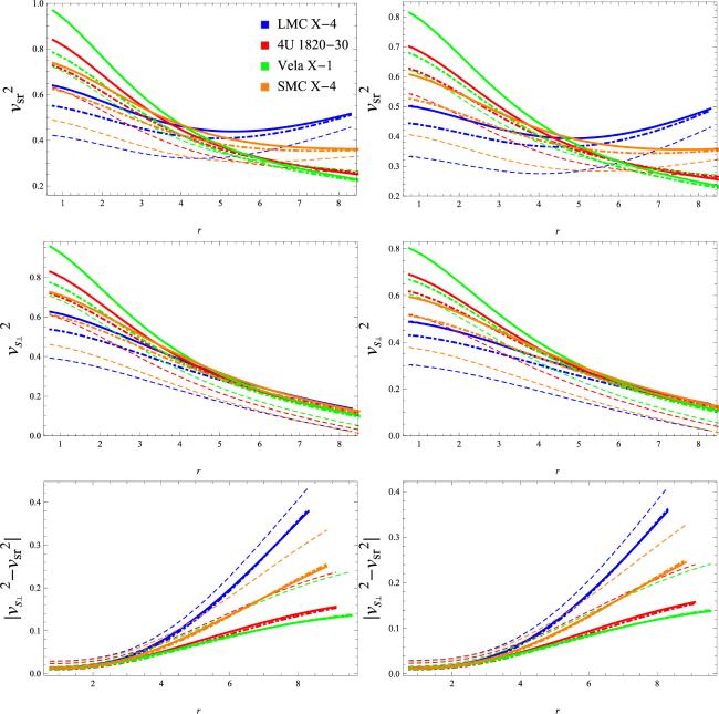
| (e)In the realm of celestial bodies, various factors can induce fluctuations, causing deviations from being in hydrostatic equilibrium state. Such deviations may lead to instability within the fluid distribution of these celestial objects, potentially affecting their long-term existence. To assess the structural stability, multiple methodologies have been proposed, with a particular focus on sound speed and perturbation techniques. An interesting and fundamental condition for the stability of a celestial body is that the speed of light must surpass the speed of sound within it. This can be expressed mathematically as $\begin{eqnarray*}0\lt {v}_{{sr}}^{2}=\displaystyle \frac{{{\rm{d}}{P}}_{r}}{{\rm{d}}\mu },\,{v}_{s\perp }^{2}=\displaystyle \frac{{{\rm{d}}{P}}_{\perp }}{{\rm{d}}\mu }\lt 1,\end{eqnarray*}$ where vsr2 is the radial speed and ${v}_{s\perp }^{2}$ represents the tangential speed of sound [76]. Additionally, Herrera [77] suggested that structural stability is maintained when the total force in the radial direction remains the same. Thus, preventing structural cracking is imperative for establishing a physically stable model. According to him, the factor $| {v}_{s\perp }^{2}-{v}_{{sr}}^{2}| $ must fall within the range of 0 to 1 to reduce the risk of instability of the considered structure. |
6. Some novel anisotropic models
6.1. Model 1

Figure 1. Deformation function ( |

Figure 2. Physical determinants (in km−2) versus r (in km) for α = 0.3 and ϖ = 0.1 (solid), α = 0.3 and ϖ = 0.9 (dotted–dashed), and α = 0.4 and ϖ = 0.9 (dashed) along with Q = 0.1 (left) and Q = 0.6 (right) corresponding to model 1. |
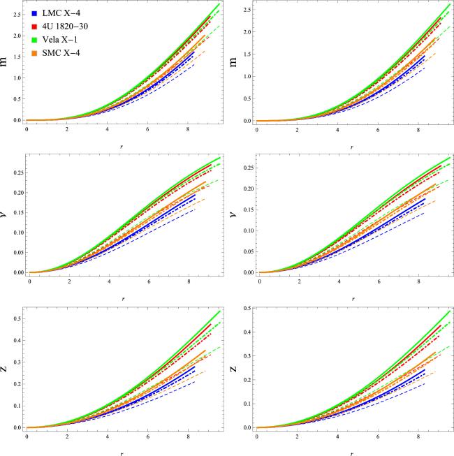
Figure 3. Mass (in km), compactness, and surface redshift versus r (in km) for α = 0.3 and ϖ = 0.1 (solid), α = 0.3 and ϖ = 0.9 (dotted–dashed), and α = 0.4 and ϖ = 0.9 (dashed) along with Q = 0.1 (left) and Q = 0.6 (right) corresponding to model 1. |

Figure 4. Energy bounds (in km−2) versus r (in km) for α = 0.3 and ϖ = 0.1 (solid), α = 0.3 and ϖ = 0.9 (dotted–dashed), and α = 0.4 and ϖ = 0.9 (dashed) along with Q = 0.1 (left) and Q = 0.6 (right) corresponding to model 1. |
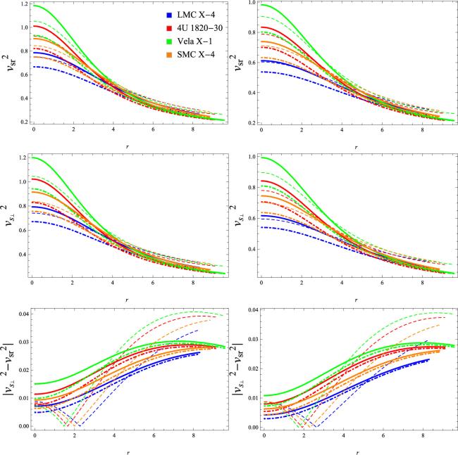
Figure 5. Stability analysis versus r (in km) for α = 0.3 and ϖ = 0.1 (solid), α = 0.3 and ϖ = 0.9 (dotted–dashed), and α = 0.4 and ϖ = 0.9 (dashed) along with Q = 0.1 (left) and Q = 0.6 (right) corresponding to model 1. |
6.2. Model 2

Figure 6. Deformation function ( |

Figure 7. Physical determinants (in km−2) versus r (in km) for α = 0.3 and ϖ = 0.1 (solid), α = 0.3 and ϖ = 0.9 (dotted–dashed), and α = 0.4 and ϖ = 0.9 (dashed) along with Q = 0.1 (left) and Q = 0.6 (right) corresponding to model 2. |

Figure 8. Mass (in km), compactness, and surface redshift versus r (in km) for α = 0.3 and ϖ = 0.1 (solid), α = 0.3 and ϖ = 0.9 (dotted–dashed), and α = 0.4 and ϖ = 0.9 (dashed) along with Q = 0.1 (left) and Q = 0.6 (right) corresponding to model 2. |
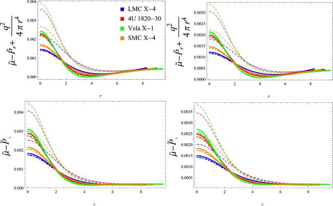
Figure 9. Energy bounds (in km−2) versus r (in km) for α = 0.3 and ϖ = 0.1 (solid), α = 0.3 and ϖ = 0.9 (dotted–dashed), and α = 0.4 and ϖ = 0.9 (dashed) along with Q = 0.1 (left) and Q = 0.6 (right) corresponding to model 2. |

Figure 10. Stability analysis versus r (in km) for α = 0.3 and ϖ = 0.1 (solid), α = 0.3 and ϖ = 0.9 (dotted–dashed), and α = 0.4 and ϖ = 0.9 (dashed) along with Q = 0.1 (left) and Q = 0.6 (right) corresponding to model 2. |
6.3. Model 3

Figure 11. Deformation function and extended component versus r (in km) for α = 0.3 and ϖ = 0.1 (solid), α = 0.3 and ϖ = 0.9 (dotted–dashed), and α = 0.4 and ϖ = 0.9 (dashed) along with Q = 0.1 (left) and Q = 0.6 (right) corresponding to model 3. |

Figure 12. Physical determinants (in km−2) versus r (in km) for α = 0.3 and ϖ = 0.1 (solid), α = 0.3 and ϖ = 0.9 (dotted–dashed), and α = 0.4 and ϖ = 0.9 (dashed) along with Q = 0.1 (left) and Q = 0.6 (right) corresponding to model 3. |
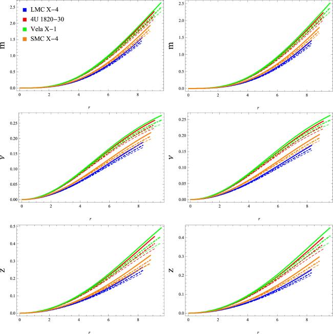
Figure 13. Mass (in km), compactness, and surface redshift versus r (in km) for α = 0.3 and ϖ = 0.1 (solid), α = 0.3 and ϖ = 0.9 (dotted–dashed), and α = 0.4 and ϖ = 0.9 (dashed) along with Q = 0.1 (left) and Q = 0.6 (right) corresponding to model 3. |
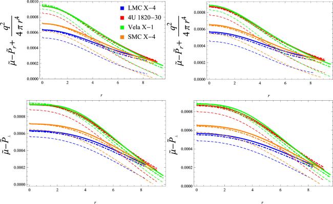
Figure 14. Energy bounds (in km−2) versus r (in km) for α = 0.3 and ϖ = 0.1 (solid), α = 0.3 and ϖ = 0.9 (dotted–dashed), and α = 0.4 and ϖ = 0.9 (dashed) along with Q = 0.1 (left) and Q = 0.6 (right) corresponding to model 3. |
Figure 15. Stability analysis versus r (in km) for α = 0.3 and ϖ = 0.1 (solid), α = 0.3 and ϖ = 0.9 (dotted–dashed), and α = 0.4 and ϖ = 0.9 (dashed) along with Q = 0.1 (left) and Q = 0.6 (right) corresponding to model 3. |