


1. Introduction
The theory of discrete integrable systems has been well studied within the past decades, leading to a large number of magnificent achievements in this field (see [1] and references therein). A key feature of the integrability of discrete systems is the phenomenon of multidimensional consistency [2, 3]. For multi-linear quadrilateral lattice equations A = B = Q = 0, this property also named consistency-around-the-cube (CAC), is usually characterized as an initial value problem, where $\widehat{\widetilde{v}}$ is determined uniquely from $u,\,\widetilde{u},\,\widehat{u},\,v$ [3–5] (see figure 1). With this property and three additional requirements (affine linear, D4 symmetry and tetrahedron property) on lattice equations1.1 ), the dependent variable u: = u(n, m) is function defined on the discrete coordinates $(n,m)\in {{\mathbb{Z}}}^{2};$ p and q are the continuous lattice parameter associated with the grid size in the n and m-directions of the lattice and we write $\widetilde{u}:= u(n+1,m)$ and $\widehat{u}:= u(n,m+1)$ for the elementary shifts in the n and m-direction of the lattice. Up to now, many methods have been applied to construct a variety of exact solutions to the H1 equation (1.2 ), including the bilinear method [9–11], Cauchy matrix approach [12, 13], inverse scattering transform [14], finite-gap integration [15], and so forth.
$\begin{eqnarray}Q(u,\widetilde{u},\widehat{u},\widehat{\widetilde{u}};p,q)=0,\end{eqnarray}$
Adler, Bobenko, and Suris (ABS) [6] got a lattice list named H1, H2, H3δ, A1δ, A2, Q1δ, Q2, Q3δ and Q4, where v is taken as $\bar{u}$. Among the list some are lattice Korteweg–de Vries (KdV) type equations [7], where H1 as the lowest equation in the list is nothing but the lattice potential KdV equation $\begin{eqnarray}{\rm{H}}1\,:\,\quad (u-\widehat{\widetilde{u}})(\widetilde{u}-\widehat{u})-p+q=0,\end{eqnarray}$
firstly appearing as the nonlinear superposition of Bäcklund transformations of the potential KdV equation [8]. In equation (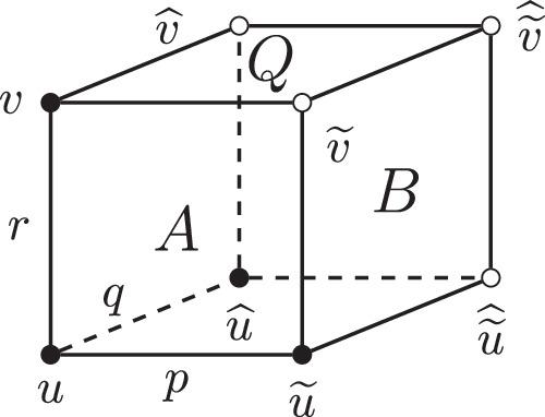
Figure 1. Consistency: quad equations can be posed on the six faces of a cube, we have A = 0 on the front and back faces, B = 0 on the left and right faces, and Q = 0 on the top and bottom faces. The black dots indicate initial values. Each equation depends on two of the three lattice parameters p, q, r. |
In the ABS classification, the scalar quadrilateral equation (1.1 ) together with its five copies defined on the other five faces compose a consistent cube, where the bottom equation and the top equation in figure 1 are, respectively, described as (1.1 ) and $(\bar{u}-\widehat{\widetilde{\bar{u}}})(\widetilde{\bar{u}}-\widehat{\bar{u}})-p+q=0$, and the equations in the front and left faces to supply the auto-Bäcklund transformation (BT). In [16], Boll extended the ABS classification and considered a more general consistent cube (e.g. the equations defined on the bottom, left and back side being different). In this case, the two equations defined on the left and front sides still compose a BT for the two equations on the bottom and on the top. Recently, a type of BTs given in [17] was interpreted as a result of the deformation of auto BTs of the ABS equations and the torqued versions of the ABS equations were obtained [18], where a torqued H1 equation is proposed1.3 ), and plane wave factor
$\begin{eqnarray}{\rm{H}}{1}^{a}\,:\,\quad (u-\widetilde{u})(\widehat{\widetilde{u}}-\widehat{u})+{p}^{2}=0.\end{eqnarray}$
This equation is referred to as nonsymmetric discrete KdV model, which composes a consistent cube together with H1 equation and Q1δ=0 in two ways [19]. In [19], BT was applied to construct a one-soliton solution for the H1a equation ( $\begin{eqnarray}\rho ={\left(\displaystyle \frac{k+p}{k-p}\right)}^{n}{\left(-1\right)}^{m}{\rho }^{0},\end{eqnarray}$
was revealed.In this paper, we would like to construct multisoliton solutions and Jordan-block solutions for the H1a equation (1.3 ) by utilizing the Cauchy matrix approach [12, 13], where the method arose from the well-known Sylvester equation in matrix theory [20] and could be viewed as a byproduct of the direct linearization method [7, 21]. The idea behind the Cauchy matrix approach, to use the determining equation set (DES) as the starting point, was developed further in a series of papers [22–29]. The paper is organized as follows. In section 2 , we describe the Cauchy matrix scheme for the H1a equation (1.3 ). In section 3 , exact solutions, including soliton solutions, Jordan-block solutions and soliton-Jordan-block mixed solutions, are constructed by solving the DES. Section 4 is for conclusions.
2. Cauchy matrix scheme for the H1a equation
We start by introducing the DES 2.1 a) is nothing but the famous Sylvester equation (SE), which has a unique solution M for given K, r and tc if ${ \mathcal E }({\boldsymbol{K}})\cap { \mathcal E }(-{\boldsymbol{K}})=\varnothing $, where ${ \mathcal E }({\boldsymbol{K}})$ represents the eigenvalue set of K. A straightforward calculation based on the DES (2.1 ) yields the following relations2.1a ) which can be thought of as the defining property of M, where and whereafter I is the N × N unit matrix.
$\begin{eqnarray}{\boldsymbol{M}}{\boldsymbol{K}}+{\boldsymbol{K}}{\boldsymbol{M}}={\boldsymbol{r}}\,{\,}^{t}{\boldsymbol{c}},\end{eqnarray}$
$\begin{eqnarray}({\boldsymbol{K}}-p{\boldsymbol{I}})\widetilde{{\boldsymbol{r}}}=({\boldsymbol{K}}+p{\boldsymbol{I}}){\boldsymbol{r}},\end{eqnarray}$
$\begin{eqnarray}\widehat{{\boldsymbol{r}}}=-{\boldsymbol{r}},\end{eqnarray}$
where ${\boldsymbol{M}}={\left({M}_{i,j}\right)}_{N\times N}$ and ${\boldsymbol{K}}={\left({k}_{i,j}\right)}_{N\times N}$ are N × N matrices, ${\boldsymbol{r}}={({\rho }_{1},{\rho }_{2},\cdots ,{\rho }_{N})}^{{\rm{T}}}$ and tc = (c1, c2, ⋯ ,cN) are Nth order column and row vectors, respectively. Here tc does not mean transpose of c but only a notation, transpose is represented by tcT. Among these matrices, Mi,j and ρj are undetermined functions of (n, m) while ki,j and cj are constants. Equation ( $\begin{eqnarray}\widetilde{{\boldsymbol{M}}}({\boldsymbol{K}}+p{\boldsymbol{I}})+({\boldsymbol{K}}+p{\boldsymbol{I}}){\boldsymbol{M}}=\widetilde{{\boldsymbol{r}}}\,{\,}^{t}{\boldsymbol{c}},\end{eqnarray}$
$\begin{eqnarray}\widehat{{\boldsymbol{M}}}{\boldsymbol{K}}-{\boldsymbol{K}}{\boldsymbol{M}}=\widehat{{\boldsymbol{r}}}\,{\,}^{t}{\boldsymbol{c}},\end{eqnarray}$
$\begin{eqnarray}({\boldsymbol{K}}-p{\boldsymbol{I}})\widetilde{{\boldsymbol{M}}}+{\boldsymbol{M}}({\boldsymbol{K}}-p{\boldsymbol{I}})={\boldsymbol{r}}{\,}^{t}{\boldsymbol{c}},\end{eqnarray}$
$\begin{eqnarray}-{\boldsymbol{K}}\widehat{{\boldsymbol{M}}}-{\boldsymbol{M}}(-{\boldsymbol{K}})={\boldsymbol{r}}{\,}^{t}{\boldsymbol{c}},\end{eqnarray}$
which encode all the information on the dynamics of the matrix M, with respect to the discrete variables n, m, in addition to (To proceed, we introduce master function2.1a ) and shift relation (2.1b ) [13]. Besides, we introduce two vector functions 2.3 ) can be expressed as2.1 ) we can derive shift relations for the master function (2.3a ), which are presented in the following proposition.
$\begin{eqnarray}{S}^{(i,j)}={\,}^{t}{\boldsymbol{c}}\,{{\boldsymbol{K}}}^{j}{\left({\boldsymbol{I}}+{\boldsymbol{M}}\right)}^{-1}{{\boldsymbol{K}}}^{i}{\boldsymbol{r}},\ \end{eqnarray}$
together with auxiliary scalar functions $\begin{eqnarray}{U}^{(i,j)}={\,}^{t}{\boldsymbol{c}}{{\boldsymbol{K}}}^{j}{\left({\boldsymbol{I}}+{\boldsymbol{M}}\right)}^{-1}({\boldsymbol{K}}-p{\boldsymbol{I}}){\left({\boldsymbol{I}}+\widetilde{{\boldsymbol{M}}}\right)}^{-1}{{\boldsymbol{K}}}^{i}\widetilde{{\boldsymbol{r}}},\end{eqnarray}$
$\begin{eqnarray}{V}^{(i,j)}={\,}^{t}{\boldsymbol{c}}{{\boldsymbol{K}}}^{j}{\left({\boldsymbol{I}}+\widetilde{{\boldsymbol{M}}}\right)}^{-1}({\boldsymbol{K}}+p{\boldsymbol{I}}){\left({\boldsymbol{I}}+{\boldsymbol{M}}\right)}^{-1}{{\boldsymbol{K}}}^{i}{\boldsymbol{r}},\end{eqnarray}$
with $i,j\in {\mathbb{Z}}$, where these functions have the symmetric property S(i,j) = S(j,i) and U(i,j) = V(j,i) thanks to the SE ( $\begin{eqnarray}{{\boldsymbol{u}}}^{(i)}={\left({\boldsymbol{I}}+{\boldsymbol{M}}\right)}^{-1}{{\boldsymbol{K}}}^{i}{\boldsymbol{r}},\quad i\in {\mathbb{Z}},\end{eqnarray}$
$\begin{eqnarray}{\,}^{t}{{\boldsymbol{u}}}^{(j)}={\,}^{t}{\boldsymbol{c}}{{\boldsymbol{K}}}^{j}{\left({\boldsymbol{I}}+{\boldsymbol{M}}\right)}^{-1},\quad j\in {\mathbb{Z}},\end{eqnarray}$
with which the functions in ( $\begin{eqnarray}\begin{array}{l}{S}^{(i,j)}={\,}^{t}{\boldsymbol{c}}\,{{\boldsymbol{K}}}^{j}{{\boldsymbol{u}}}^{(i)}={\,}^{t}{{\boldsymbol{u}}}^{(j)}{{\boldsymbol{K}}}^{i}{\boldsymbol{r}},\\ {U}^{(i,j)}={\,}^{t}{{\boldsymbol{u}}}^{(j)}({\boldsymbol{K}}-p{\boldsymbol{I}}){\widetilde{{\boldsymbol{u}}}}^{(i)},\\ {V}^{(i,j)}={\widetilde{{\,}^{t}{\boldsymbol{u}}}}^{(j)}({\boldsymbol{K}}+p{\boldsymbol{I}}){{\boldsymbol{u}}}^{(i)}.\end{array}\end{eqnarray}$
It is easy to find the functions S(i,j), U(i,j) and V(i,j) are invariant under similarity transformation [13]. By the DES (For the matrices ${\boldsymbol{M}},{\boldsymbol{K}}$ and vectors ${\boldsymbol{r}},{\,}^{t}{\boldsymbol{c}}$ obeying the DES (
$\begin{eqnarray}\begin{array}{l}{\widetilde{S}}^{(i,j+1)}-p{\widetilde{S}}^{(i,j)}=2{U}^{(i,j)}-{S}^{(i+1,j)}\\ -{{pS}}^{(i,j)}+{\widetilde{S}}^{(i,0)}{S}^{(0,j)},\end{array}\end{eqnarray}$
$\begin{eqnarray}\begin{array}{l}{S}^{(i,j+1)}+{{pS}}^{(i,j)}=2{V}^{(i,j)}-{\widetilde{S}}^{(i+1,j)}\\ +p{\widetilde{S}}^{(i,j)}+{S}^{(i,0)}{\widetilde{S}}^{(0,j)},\end{array}\end{eqnarray}$
$\begin{eqnarray}{\widehat{S}}^{(i,j+1)}={S}^{(0,j)}{\widehat{S}}^{(i,0)}-{S}^{(i+1,j)},\end{eqnarray}$
$\begin{eqnarray}{S}^{(i,j+1)}={S}^{(i,0)}{\widehat{S}}^{(0,j)}-{\widehat{S}}^{(i+1,j)}.\end{eqnarray}$
We just pay attention to the relation (
$\begin{eqnarray}({\boldsymbol{I}}+{\boldsymbol{M}}){{\boldsymbol{u}}}^{(i)}={{\boldsymbol{K}}}^{i}{\boldsymbol{r}}.\end{eqnarray}$
Taking $\widetilde{}$-shift of ( $\begin{eqnarray}\begin{array}{l}{{\boldsymbol{K}}}^{i}({\boldsymbol{K}}+p{\boldsymbol{I}}){\boldsymbol{r}}=2({\boldsymbol{K}}-p{\boldsymbol{I}}){\widetilde{{\boldsymbol{u}}}}^{(i)}\\ -({\boldsymbol{I}}+{\boldsymbol{M}})({\boldsymbol{K}}-p{\boldsymbol{I}}){\widetilde{{\boldsymbol{u}}}}^{(i)}+{\widetilde{S}}^{(i,0)}{\boldsymbol{r}},\end{array}\end{eqnarray}$
where we have used the relation ( $\begin{eqnarray}\begin{array}{l}({\boldsymbol{K}}-p{\boldsymbol{I}}){\widetilde{{\boldsymbol{u}}}}^{(i)}=2{\left({\boldsymbol{I}}+{\boldsymbol{M}}\right)}^{-1}({\boldsymbol{K}}-p{\boldsymbol{I}}){\widetilde{{\boldsymbol{u}}}}^{(i)}\\ -{{\boldsymbol{u}}}^{(i+1)}-p{{\boldsymbol{u}}}^{(i)}+{\widetilde{S}}^{(i,0)}{{\boldsymbol{u}}}^{(0)}.\end{array}\end{eqnarray}$
Left-multiplying (We next to construct the H1a equation (1.3 ). For the sake of simplicity, we define w = S(0,0), v = U(0,0) = V(0,0). Let i = j = 0, then relations (2.6 ) give rise to2.1b ) and (2.1c ), from (2.10a ) and its hat-version we obtain2.2a ) is adopted. From a comparison of (2.11 ) with (2.12 ), it follows that a closed-form equation in terms of w:2.13 ), we obtain torqued H1a equation2.1 ).
$\begin{eqnarray}{\widetilde{S}}^{(\mathrm{0,1})}-p\widetilde{w}=2v-{S}^{(\mathrm{0,1})}-{pw}+\widetilde{w}w,\end{eqnarray}$
$\begin{eqnarray}{\widehat{S}}^{(\mathrm{0,1})}=w\widehat{w}-{S}^{(\mathrm{0,1})},\end{eqnarray}$
where the symmetric relation S(1,0) = S(0,1) is used. On one hand, removing variable S(0,1) yields $\begin{eqnarray}2(v+\widehat{v})=p(w+\widehat{w}-\widetilde{w}-\widehat{\widetilde{w}})-(\widetilde{w}-\widehat{w})(w-\widehat{\widetilde{w}}).\end{eqnarray}$
On the other hand, noticing ( $\begin{eqnarray}\begin{array}{l}2(v+\widehat{v})={\widetilde{S}}^{(\mathrm{0,1})}-p\widetilde{w}+{S}^{(\mathrm{0,1})}+{pw}+{\widehat{\widetilde{S}}}^{(\mathrm{0,1})}-p\widehat{\widetilde{w}}+{\widehat{S}}^{(\mathrm{1,0})}+p\widehat{w}-\widetilde{w}w-\widehat{\widetilde{w}}\widehat{w}\\ ={\,}^{t}{\boldsymbol{c}}{\left({\boldsymbol{I}}+\widetilde{{\boldsymbol{M}}}\right)}^{-1}({\boldsymbol{K}}+p{\boldsymbol{I}}){\boldsymbol{r}}+{\,}^{t}{\boldsymbol{c}}({\boldsymbol{K}}+p{\boldsymbol{I}}){\left({\boldsymbol{I}}+{\boldsymbol{M}}\right)}^{-1}{\boldsymbol{r}}\\ \quad -{\,}^{t}{\boldsymbol{c}}{\left({\boldsymbol{I}}+\widehat{\widetilde{{\boldsymbol{M}}}}\right)}^{-1}({\boldsymbol{K}}+p{\boldsymbol{I}}){\boldsymbol{r}}-{\,}^{t}{\boldsymbol{c}}({\boldsymbol{K}}+p{\boldsymbol{I}}){\left({\boldsymbol{I}}+\widehat{{\boldsymbol{M}}}\right)}^{-1}{\boldsymbol{r}}-\widetilde{w}w-\widehat{\widetilde{w}}\widehat{w}\\ ={\,}^{t}{\boldsymbol{c}}\,[{\left({\boldsymbol{I}}+\widetilde{{\boldsymbol{M}}}\right)}^{-1}({\boldsymbol{K}}+p{\boldsymbol{I}})({\boldsymbol{I}}+\widehat{{\boldsymbol{M}}}){\left({\boldsymbol{I}}+\widehat{{\boldsymbol{M}}}\right)}^{-1}-{\left({\boldsymbol{I}}+\widehat{\widetilde{{\boldsymbol{M}}}}\right)}^{-1}({\boldsymbol{K}}+p{\boldsymbol{I}})({\boldsymbol{I}}+{\boldsymbol{M}}){\left({\boldsymbol{I}}+{\boldsymbol{M}}\right)}^{-1}\\ \quad +{\left({\boldsymbol{I}}+\widehat{\widetilde{{\boldsymbol{M}}}}\right)}^{-1}({\boldsymbol{I}}+\widehat{\widetilde{{\boldsymbol{M}}}})({\boldsymbol{K}}+p{\boldsymbol{I}}){\left({\boldsymbol{I}}+{\boldsymbol{M}}\right)}^{-1}-{\left({\boldsymbol{I}}+\widetilde{{\boldsymbol{M}}}\right)}^{-1}({\boldsymbol{I}}+\widetilde{{\boldsymbol{M}}})({\boldsymbol{K}}+p{\boldsymbol{I}}){\left({\boldsymbol{I}}+\widehat{{\boldsymbol{M}}}\right)}^{-1}]{\boldsymbol{r}}\\ \quad -\widetilde{w}w-\widehat{\widetilde{w}}\widehat{w}\\ ={\,}^{t}{\boldsymbol{c}}\,[-{\left({\boldsymbol{I}}+\widetilde{{\boldsymbol{M}}}\right)}^{-1}({\boldsymbol{K}}+p{\boldsymbol{I}}){\boldsymbol{M}}{\left({\boldsymbol{I}}+\widehat{{\boldsymbol{M}}}\right)}^{-1}-{\left({\boldsymbol{I}}+\widetilde{{\boldsymbol{M}}}\right)}^{-1}\widetilde{{\boldsymbol{M}}}({\boldsymbol{K}}+p{\boldsymbol{I}}){\left({\boldsymbol{I}}+\widehat{{\boldsymbol{M}}}\right)}^{-1}\\ \quad -{\left({\boldsymbol{I}}+\widehat{\widetilde{{\boldsymbol{M}}}}\right)}^{-1}\widetilde{{\boldsymbol{M}}}({\boldsymbol{K}}+p{\boldsymbol{I}}){\left({\boldsymbol{I}}+{\boldsymbol{M}}\right)}^{-1}-{\left({\boldsymbol{I}}+\widehat{\widetilde{{\boldsymbol{M}}}}\right)}^{-1}({\boldsymbol{K}}+p{\boldsymbol{I}}){\boldsymbol{M}}{\left({\boldsymbol{I}}+{\boldsymbol{M}}\right)}^{-1}]{\boldsymbol{r}}-\widetilde{w}w-\widehat{\widetilde{w}}\widehat{w}\\ ={\,}^{t}{\boldsymbol{c}}\,[-{\left({\boldsymbol{I}}+\widetilde{{\boldsymbol{M}}}\right)}^{-1}(\widetilde{{\boldsymbol{M}}}({\boldsymbol{K}}+p{\boldsymbol{I}})+({\boldsymbol{K}}+p{\boldsymbol{I}}){\boldsymbol{M}}){\left({\boldsymbol{I}}+\widehat{{\boldsymbol{M}}}\right)}^{-1}\\ \quad -{\left({\boldsymbol{I}}+\widehat{\widetilde{{\boldsymbol{M}}}}\right)}^{-1}(\widetilde{{\boldsymbol{M}}}({\boldsymbol{K}}+p{\boldsymbol{I}})+({\boldsymbol{K}}+p{\boldsymbol{I}}){\boldsymbol{M}}){\left({\boldsymbol{I}}+{\boldsymbol{M}}\right)}^{-1}]{\boldsymbol{r}}-\widetilde{w}w-\widehat{\widetilde{w}}\widehat{w}\\ ={\,}^{t}{\boldsymbol{c}}\,[-{\left({\boldsymbol{I}}+\widetilde{{\boldsymbol{M}}}\right)}^{-1}\widetilde{{\boldsymbol{r}}}{\,}^{t}{\boldsymbol{c}}{\left({\boldsymbol{I}}+\widehat{{\boldsymbol{M}}}\right)}^{-1}-{\left({\boldsymbol{I}}+\widehat{\widetilde{{\boldsymbol{M}}}}\right)}^{-1}\widetilde{{\boldsymbol{r}}}{\,}^{t}{\boldsymbol{c}}{\left({\boldsymbol{I}}+{\boldsymbol{M}}\right)}^{-1}]{\boldsymbol{r}}-\widetilde{w}w-\widehat{\widetilde{w}}\widehat{w}\\ ={\,}^{t}{\boldsymbol{c}}{\left({\boldsymbol{I}}+\widetilde{{\boldsymbol{M}}}\right)}^{-1}\widetilde{{\boldsymbol{r}}}{\,}^{t}{\boldsymbol{c}}{\left({\boldsymbol{I}}+\widehat{{\boldsymbol{M}}}\right)}^{-1}\widehat{{\boldsymbol{r}}}+{\,}^{t}{\boldsymbol{c}}{\left({\boldsymbol{I}}+\widehat{\widetilde{{\boldsymbol{M}}}}\right)}^{-1}\widehat{\widetilde{{\boldsymbol{r}}}}{\,}^{t}{\boldsymbol{c}}{\left({\boldsymbol{I}}+{\boldsymbol{M}}\right)}^{-1}{\boldsymbol{r}}-\widetilde{w}w-\widehat{\widetilde{w}}\widehat{w}\\ =\widetilde{w}\widehat{w}+\widehat{\widetilde{w}}w-\widetilde{w}w-\widehat{\widetilde{w}}\widehat{w},\end{array}\end{eqnarray}$
where equation ( $\begin{eqnarray}(p+w-\widetilde{w})(p+\widehat{w}-\widehat{\widetilde{w}})-{p}^{2}=0.\end{eqnarray}$
Inserting the point transformation u = w − np − qm − c (c is a constant) into ( $\begin{eqnarray}(u-\widetilde{u})(\widehat{\widetilde{u}}-\widehat{u})-{p}^{2}=0,\end{eqnarray}$
whose solution is given by $\begin{eqnarray}u={\,}^{t}{\boldsymbol{c}}{\left({\boldsymbol{I}}+{\boldsymbol{M}}\right)}^{-1}{\boldsymbol{r}}-{np}-{qm}-c,\end{eqnarray}$
where matrices tc, M and r satisfy the DES (3. Exact solutions
The main result of the paper [19] was to give the one-soliton solution for equation (2.14 ), however, without presenting multisoliton solutions. To exhibit exact solutions of the torqued H1a equation, we just need to solve the DES (2.1 ). Since it is covariant under similarity transformation, we turn to solve the canonical DES
$\begin{eqnarray}{\boldsymbol{M}}{\boldsymbol{\Gamma }}+{\boldsymbol{\Gamma }}{\boldsymbol{M}}={\boldsymbol{r}}\,{\,}^{t}{\boldsymbol{c}},\end{eqnarray}$
$\begin{eqnarray}({\boldsymbol{\Gamma }}-p{\boldsymbol{I}})\widetilde{{\boldsymbol{r}}}=({\boldsymbol{\Gamma }}+p{\boldsymbol{I}}){\boldsymbol{r}},\end{eqnarray}$
$\begin{eqnarray}\widehat{{\boldsymbol{r}}}=-{\boldsymbol{r}},\end{eqnarray}$
where Γ is the Jordan canonical matrix of K and satisfies ${ \mathcal E }({\boldsymbol{\Gamma }})\cap { \mathcal E }(-{\boldsymbol{\Gamma }})=\varnothing $. In virtue of the canonical structure of Γ, it is possible to give a complete classification for the solutions. The procedure follows the method shown in [13], where the matrix M was factorized as M = FGH.3.1. List of notations
We firstly list some main notations, where the subscripts D and J usually correspond to the cases of Γ being diagonal and being Jordan-block, respectively.
$\begin{eqnarray}{\rm{plane}}\,{\rm{wave}}\,{\rm{factor}}:\,\,{\rho }_{i}={\left(\displaystyle \frac{{k}_{i}+p}{{k}_{i}-p}\right)}^{n}{\left(-1\right)}^{m}{\rho }_{i}^{0},\end{eqnarray}$
$\begin{eqnarray}N{\rm{th}}\,{\rm{order}}\,{\rm{vector}}:\,\,{{\boldsymbol{r}}}_{D}^{\left[N\right]}({\left\{{k}_{i}\right\}}_{1}^{N})={\left({\rho }_{1},{\rho }_{2},\cdots ,{\rho }_{N}\right)}^{{\rm{T}}},\end{eqnarray}$
$\begin{eqnarray}N{\rm{th}}\,{\rm{order}}\,{\rm{vector}}:\,\,{{\boldsymbol{r}}}_{J}^{\left[N\right]}({k}_{1})={\left({\rho }_{1},\displaystyle \frac{{{\rm{\partial }}}_{{k}_{1}}{\rho }_{1}}{1!},\cdots ,\displaystyle \frac{{{\rm{\partial }}}_{{k}_{1}}^{N-1}{\rho }_{1}}{\left(N-1)!\right.}\right)}^{{\rm{T}}},\end{eqnarray}$
$\begin{eqnarray}N\times N\,\mathrm{matrix}:\,\,{{\boldsymbol{\Gamma }}}_{D}^{[N]}({\{{k}_{i}\}}_{1}^{N})=\mathrm{Diag}({k}_{1},{k}_{2},\cdots ,{k}_{N}),\end{eqnarray}$
$\begin{eqnarray}N\times N\,\mathrm{matrix}:\,\,{{\boldsymbol{\Gamma }}}_{J}^{[N]}(a)=\left(\begin{array}{cccccc}a & 0 & 0 & \cdots & 0 & 0\\ 1 & a & 0 & \cdots & 0 & 0\\ 0 & 1 & a & \cdots & 0 & 0\\ \vdots & \vdots & \vdots & \vdots & \vdots & \vdots \\ 0 & 0 & 0 & \cdots & 1 & a\end{array}\right),\end{eqnarray}$
$\begin{eqnarray}N\times N\,\mathrm{matrix}:\,\,{{\boldsymbol{F}}}_{D}^{[N]}({\{{k}_{i}\}}_{1}^{N})=\mathrm{Diag}({\rho }_{1},{\rho }_{2},\cdots ,{\rho }_{N}),\end{eqnarray}$
$\begin{eqnarray}N\times N\,\mathrm{matrix}:\,\,{{\boldsymbol{H}}}_{D}^{[N]}(\{{c}_{i}\}{}_{1}^{N})=\mathrm{Diag}({c}_{1},{c}_{2},\cdots ,{c}_{N}),\end{eqnarray}$
$\begin{eqnarray}N\times N\,\mathrm{matrix}:\,\,{{\boldsymbol{F}}}_{J}^{[N]}({k}_{1})=\left(\begin{array}{ccccc}{\rho }_{1} & 0 & 0 & \cdots & 0\\ \displaystyle \frac{{\partial }_{{k}_{1}}{\rho }_{1}}{1!} & {\rho }_{1} & 0 & \cdots & 0\\ \displaystyle \frac{{\partial }_{{k}_{1}}^{2}{\rho }_{1}}{2!} & \displaystyle \frac{{\partial }_{{k}_{1}}{\rho }_{1}}{1!} & {\rho }_{1} & \cdots & 0\\ \vdots & \vdots & \vdots & \ddots & \vdots \\ \displaystyle \frac{{\partial }_{{k}_{1}}^{N-1}{\rho }_{1}}{(N-1)!} & \displaystyle \frac{{\partial }_{{k}_{1}}^{N-2}{\rho }_{1}}{(N-2)!} & \displaystyle \frac{{\partial }_{{k}_{1}}^{N-3}{\rho }_{1}}{(N-3)!} & \cdots & {\rho }_{1}\end{array}\right),\end{eqnarray}$
$\begin{eqnarray}N\times N\,\mathrm{matrix}:\,\,{{\boldsymbol{H}}}_{J}^{[N]}(\{{c}_{i}\}{}_{1}^{N})=\left(\begin{array}{ccccc}{c}_{1} & \cdots & {c}_{N-2} & {c}_{N-1} & {c}_{N}\\ {c}_{2} & \cdots & {c}_{N-1} & {c}_{N} & 0\\ {c}_{3} & \cdots & {c}_{N} & 0 & 0\\ \vdots & \vdots & \vdots & \vdots & \vdots \\ {c}_{N} & \cdots & 0 & 0 & 0\end{array}\right),\end{eqnarray}$
$\begin{eqnarray}N\times N\,\mathrm{matrix}:\,\,{{\boldsymbol{G}}}_{D}^{[N]}({\{{k}_{i}\}}_{1}^{N})={\left({g}_{i,j}\right)}_{N\times N},\,\,\,{g}_{i,j}=\displaystyle \frac{1}{{k}_{i}+{k}_{j}},\end{eqnarray}$
$\begin{eqnarray}\begin{array}{l}{N}_{1}\times {N}_{2}\,\mathrm{matrix}:\,\,{{\boldsymbol{G}}}_{{DJ}}^{\left[{N}_{1},{N}_{2}\right]}({\{{k}_{i}\}}_{1}^{{N}_{1}};a)\\ ={\left({g}_{i,j}\right)}_{{N}_{1}\times {N}_{2}},\,\,\,{g}_{i,j}=-{\left(\displaystyle \frac{-1}{{k}_{i}+a}\right)}^{j},\end{array}\end{eqnarray}$
$\begin{eqnarray}\begin{array}{l}{N}_{1}\times {N}_{2}\,\mathrm{matrix}:\,\,{{\boldsymbol{G}}}_{{JJ}}^{\left[{N}_{1},{N}_{2}\right]}(a;b)\\ ={\left({g}_{i,j}\right)}_{{N}_{1}\times {N}_{2}},\,\,\,{g}_{i,j}={{\rm{C}}}_{i+j-2}^{i-1}\displaystyle \frac{{\left(-1\right)}^{i+j}}{{\left(a+b\right)}^{i+j-1}},\end{array}\end{eqnarray}$
$\begin{eqnarray}\begin{array}{l}N\times N\,\mathrm{matrix}:\,\,{{\boldsymbol{G}}}_{J}^{\left[N\right]}(a)={{\boldsymbol{G}}}_{{JJ}}^{\left[N,N\right]}(a;a)\\ ={\left({g}_{i,j}\right)}_{N\times N},\,\,\,{g}_{i,j}={{\rm{C}}}_{i+j-2}^{i-1}\displaystyle \frac{{\left(-1\right)}^{i+j}}{{\left(2a\right)}^{i+j-1}},\end{array}\end{eqnarray}$
where $\begin{eqnarray*}{{\rm{C}}}_{j}^{i}=\displaystyle \frac{j!}{i!(j-i)!},\,\,(j\geqslant i).\end{eqnarray*}$
The Nth order matrix in the following form $\begin{eqnarray}{ \mathcal A }={\left(\begin{array}{cccccc}{a}_{0} & 0 & 0 & \cdots & 0 & 0\\ {a}_{1} & {a}_{0} & 0 & \cdots & 0 & 0\\ {a}_{2} & {a}_{1} & {a}_{0} & \cdots & 0 & 0\\ \vdots & \vdots & \cdots & \vdots & \vdots & \vdots \\ {a}_{N-1} & {a}_{N-2} & {a}_{N-3} & \cdots & {a}_{1} & {a}_{0}\end{array}\right)}_{N\times N}\end{eqnarray}$
with scalar elements {ai} is an Nth-order lower triangular Toeplitz matrix. All such matrices compose a commutative set ${\widetilde{G}}^{\left[N\right]}$ with respect to matrix multiplication and the subset $\begin{eqnarray*}{G}^{\left[N\right]}=\left\{{ \mathcal A }| { \mathcal A }\in {\widetilde{G}}^{\left[N\right]},| { \mathcal A }| \,\ne \,0\right\}\end{eqnarray*}$
is an Abelian group. Such kind of matrices play useful roles in the expression of exact solution for soliton equations [30, 31].3.2. Solutions of the canonical DES (3.1 )
In terms of three forms of Γ: diagonal, Jordan-block, and diagonal-Jordan-block mixed form, in what follows we list solitons, Jordan-block solutions and diagonal-Jordan-block mixed solutions, respectively.
(1). When Γ being diagonal form:
$\begin{eqnarray}{\boldsymbol{\Gamma }}={{\boldsymbol{\Gamma }}}_{D}^{\left[N\right]}({\{{k}_{i}\}}_{1}^{N}),\end{eqnarray}$
we have $\begin{eqnarray}{\boldsymbol{r}}={{\boldsymbol{r}}}_{D}^{\left[N\right]}({\{{k}_{i}\}}_{1}^{N}),\quad {\boldsymbol{M}}={\boldsymbol{F}}{\boldsymbol{G}}{\boldsymbol{H}},\end{eqnarray}$
where $\begin{eqnarray}\begin{array}{l}{\boldsymbol{F}}={{\boldsymbol{F}}}_{D}^{\left[N\right]}({\{{k}_{i}\}}_{1}^{N}),\\ {\boldsymbol{G}}={{\boldsymbol{G}}}_{D}^{\left[N\right]}({\{{k}_{i}\}}_{1}^{N}),\\ {\boldsymbol{H}}={{\boldsymbol{H}}}_{D}^{\left[N\right]}(\{{c}_{i}\}{}_{1}^{N}).\end{array}\end{eqnarray}$
(2). When Γ being Jordan-block form: $\begin{eqnarray}{\boldsymbol{\Gamma }}={{\boldsymbol{\Gamma }}}_{J}^{\left[N\right]}({k}_{1}),\end{eqnarray}$
we have $\begin{eqnarray}{\boldsymbol{r}}={{\boldsymbol{r}}}_{J}^{\left[N\right]}({k}_{1}),\quad {\boldsymbol{M}}={\boldsymbol{F}}{\boldsymbol{G}}{\boldsymbol{H}},\end{eqnarray}$
where $\begin{eqnarray}\begin{array}{l}{\boldsymbol{F}}={{\boldsymbol{F}}}_{J}^{\left[N\right]}({k}_{1}),\quad {\boldsymbol{G}}={{\boldsymbol{G}}}_{J}^{\left[N\right]}({k}_{1}),\\ {\boldsymbol{H}}={{\boldsymbol{H}}}_{J}^{\left[N\right]}(\{{c}_{i}\}{}_{1}^{N}).\end{array}\end{eqnarray}$
(3). When Γ being diagonal-Jordan-block mixed form: $\begin{eqnarray}\begin{array}{l}{\boldsymbol{\Gamma }}=\mathrm{Diag}\left({{\boldsymbol{\Gamma }}}_{D}^{\left[{N}_{1}\right]}({\{{k}_{i}\}}_{1}^{{N}_{1}}),{{\boldsymbol{\Gamma }}}_{J}^{\left[{N}_{2}\right]}({k}_{{N}_{1}+1}),\right.\\ \left.{{\boldsymbol{\Gamma }}}_{J}^{\left[{N}_{3}\right]}({k}_{{N}_{1}+2}),\cdots ,{{\boldsymbol{\Gamma }}}_{J}^{\left[{N}_{s}\right]}({k}_{{N}_{1}+(s-1)})\right),\end{array}\end{eqnarray}$
where ${\sum }_{j=1}^{s}{N}_{j}=N$, we have $\begin{eqnarray}\begin{array}{l}{\boldsymbol{r}}=\left(\begin{array}{l}{{\boldsymbol{r}}}_{D}^{\left[{N}_{1}\right]}({\{{k}_{i}\}}_{1}^{{N}_{1}})\\ {{\boldsymbol{r}}}_{J}^{\left[{N}_{2}\right]}({k}_{{N}_{1}+1})\\ {{\boldsymbol{r}}}_{J}^{\left[{N}_{3}\right]}({k}_{{N}_{1}+2})\\ \vdots \\ {{\boldsymbol{r}}}_{J}^{\left[{N}_{s}\right]}({k}_{{N}_{1}+(s-1)})\end{array}\right),\quad {\boldsymbol{M}}={\boldsymbol{F}}{\boldsymbol{G}}{\boldsymbol{H}},\end{array}\end{eqnarray}$
in which $\begin{eqnarray}\begin{array}{l}{\boldsymbol{F}}=\mathrm{Diag}\left({{\boldsymbol{F}}}_{D}^{\left[{N}_{1}\right]}({\{{k}_{i}\}}_{1}^{{N}_{1}}),{{\boldsymbol{F}}}_{J}^{\left[{N}_{2}\right]}({k}_{{N}_{1}+1}),\cdots ,\right.\\ \left.{{\boldsymbol{F}}}_{J}^{\left[{N}_{s}\right]}({k}_{{N}_{1}+(s-1)})\right),\end{array}\end{eqnarray}$
$\begin{eqnarray}\begin{array}{l}{\boldsymbol{H}}=\mathrm{Diag}\left(\Space{0ex}{5.25ex}{0ex}{{\boldsymbol{H}}}_{D}^{\left[{N}_{1}\right]}(\{{c}_{i}\}{}_{1}^{{N}_{1}}),{{\boldsymbol{H}}}_{J}^{\left[{N}_{2}\right]}(\{{c}_{i}\}{}_{{N}_{1}+1}^{{N}_{1}+{N}_{2}}),\cdots ,\right.\\ \left.{{\boldsymbol{H}}}_{J}^{\left[{N}_{s}\right]}\Space{0ex}{0.25ex}{0ex}(\{{c}_{i}\}{}_{1+\displaystyle \sum _{j=1}^{s-1}{N}_{j}}^{N}\Space{0ex}{0.25ex}{0ex})\right),\end{array}\end{eqnarray}$
and G is a symmetric matrix with block structure $\begin{eqnarray}{\boldsymbol{G}}={{\boldsymbol{G}}}^{{\rm{T}}}={\left({{\boldsymbol{G}}}_{i,j}\right)}_{s\times s},\end{eqnarray}$
where $\begin{eqnarray}\begin{array}{l}{{\boldsymbol{G}}}_{\mathrm{1,1}}={{\boldsymbol{G}}}_{D}({\{{k}_{i}\}}_{1}^{{N}_{1}}),\,\\ {{\boldsymbol{G}}}_{1,j}={{\boldsymbol{G}}}_{j,1}^{{\rm{T}}}={{\boldsymbol{G}}}_{{DJ}}^{\left[{N}_{1},{N}_{j}\right]}({\{{k}_{i}\}}_{1}^{{N}_{1}};{k}_{{N}_{j-1}+1}),\,\,(1\lt i\leqslant s),\\ {{\boldsymbol{G}}}_{i,j}={{\boldsymbol{G}}}_{j,i}^{{\rm{T}}}={{\boldsymbol{G}}}_{{JJ}}^{\left[{N}_{i},{N}_{j}\right]}({k}_{{N}_{i-1}+1};{k}_{{N}_{j-1}+1}),\,\,(1\lt i\leqslant j\leqslant s).\end{array}\end{eqnarray}$
We take one-soliton, two-soliton and the simplest Jordan-block solution as examples to show the explicit form of the obtained solutions. For the sake of simplicity, we introduce the following notations
$\begin{eqnarray}\begin{array}{l}{\rho }_{{ij}}={\rho }_{i}{c}_{j},\quad {{\rm{e}}}^{{A}_{12}}={\left(\displaystyle \frac{{k}_{1}-{k}_{2}}{{k}_{1}+{k}_{2}}\right)}^{2},\\ {\eta }_{1}=\displaystyle \frac{2{np}}{{p}^{2}-{k}_{1}^{2}}.\end{array}\end{eqnarray}$
In the case of Γ = k1, we have $\begin{eqnarray}w=\displaystyle \frac{2{k}_{1}{\rho }_{11}}{2{k}_{1}+{\rho }_{11}}.\end{eqnarray}$
In the case of Γ = Diag(k1, k2), the corresponding solution reads $\begin{eqnarray}w=\displaystyle \frac{4{k}_{1}{k}_{2}({\rho }_{11}+{\rho }_{22})+2({k}_{1}+{k}_{2}){e}^{{A}_{12}}{\rho }_{11}{\rho }_{22}}{4{k}_{1}{k}_{2}+2{k}_{2}{\rho }_{11}+2{k}_{1}{\rho }_{22}+{e}^{{A}_{12}}{\rho }_{11}{\rho }_{22}}.\end{eqnarray}$
In the case of ${\boldsymbol{\Gamma }}=\left(\begin{array}{cc}{k}_{1} & 0\\ 1 & {k}_{1}\end{array}\right)$, we get the simplest Jordan-block solution $\begin{eqnarray}w=\displaystyle \frac{16{k}_{1}^{4}({\rho }_{11}+{\eta }_{1}{\rho }_{12})-4{k}_{1}{\rho }_{12}^{2}}{16{k}_{1}^{4}+8{k}_{1}^{3}({\rho }_{11}+{\eta }_{1}{\rho }_{12})-8{k}_{1}^{2}{\rho }_{12}-{\rho }_{12}^{2}}.\end{eqnarray}$
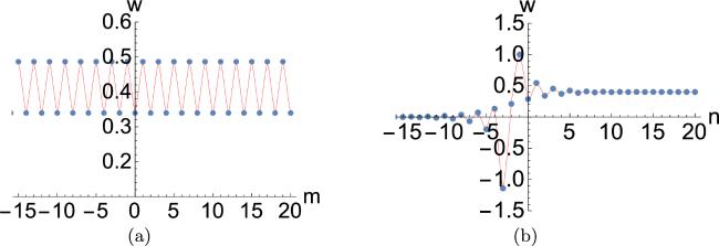
For fixed n, w in (3.11 ) takes two constant values along the m-direction, possessing a jumping property and demonstrating periodic structure (see figure 2(a)). Figure 2 depicts the behavior of solution w in (3.11 ). The two-soliton solution (3.12 ) and Jordan-block solution (3.13 ) also have these properties.
Figure 2. One-soliton solution w given by ( |
4. Conclusions
Different from the H1 equation, the H1a is referred to as a nonsymmetric version of the discrete KdV equation, and only one lattice parameter p is involved in this equation. In this paper, starting from the DES (2.1 ) we define master functions S(i,j) together with two auxiliary functions U(i,j) and V(i,j), which satisfy symmetric properties S(i,j) = S(j,i) and U(i,j) = V(j,i), as well as shift relations (2.6 ). In these four relations, equations (2.6b ) and (2.6 d) can be deduced from (2.6a ) and (2.6c ) by the symmetric properties mentioned, respectively. Compared with the usual Cauchy matrix scheme for the H1 equation, here auxiliary functions U(i,j) and V(i,j) are indispensable. Furthermore, we introduce the dependent variable w = S(0,0) and delete redundant variables from relations (2.10 ) and finally derive the H1a equation as closed-form. By solving the canonical DES (3.1 ), soliton solutions, Jordan-block solutions and mixed soliton-Jordan-block solutions are discussed, where the explicit one-soliton, two-solitons, and the simplest Jordan-block solutions are listed.
We end the paper with the following remarks. First of all, the explicit degeneration relationships among the ABS lattice list [12] enable one to construct a variety of exact solutions to the whole ABS lattice list except for the elliptic case of Q4 [11–13, 32]. While for the torqued ABS lattice list, the existence of analogous degeneration relationships is still an open question. What is more, for the H1a and H2a equations, they have different plane wave factors [19, 33]. How to discuss the whole torqued ABS lattice list in a unified Cauchy matrix scheme is an interesting question and worthy to be considered. In addition, the solutions given in the present paper can be viewed as semi-oscillatory solutions [29] since the form of plane wave factor. These types of solutions jump between two constant values for fixed n and demonstrate periodic structure. Finally, as in the continuous case, oscillatory factors ((−1)n, (−1)m) break differentiability and do not appear in analytic solutions, there is no continuum limit for the torqued H1a equation.