


1. Introduction
Recently, soliton theory has been widely studied and applied in almost all branches of physics like condensed matter physics, quantum field theory, fluid dynamics and nonlinear optics. One of the most important research fields in soliton theory is to seek for exact solutions of nonlinear evolution equations (NLEEs) [1–10]. In (2+1)-dimensions, the possible types of coherent structures represented by exact solutions like the dromions, lumps, ring solitons, breathers, instantons, compactons have been studied well. These studies are restricted to the single-valued situations. For more complicated cases, multivalued-functions also have been used to construct folded solitary waves and foldons.
It is well known that the Fourier transform and variable separation approach are the two most efficient methods for solving linear equations. The famous inverse scattering transformation (IST) can be considered as a nonlinear extension of the Fourier transformation. However, it is difficult to extend the variable separation approach to the nonlinear case consistently. Fortunately, the multilinear variable separation (MLVS) approach has been developed well for various (2+1)-dimensional integrable systems such as the Davey–Stewartson system, Nizhnik–Novikov–Veselov (NNV) system, Broe–Kaup–Kupershmidt system, special Toda equation [11–19]. Thus, there is an important problem that should be studied further for this MLVS approach. Namely, how many or what kinds of NLEEs are suitable to be solved by the MLVS approach?
Let us give a brief account of the MLVS approach. For a given (2+1)-dimensional NLEE,
$\begin{eqnarray*}{\rm{\Phi }}(u,{u}_{x},{u}_{y},{u}_{t},{u}_{{xx}},\cdots )=0,\end{eqnarray*}$
we construct a suitable auto-Bäcklund transformation firstly by means of Painlevé analysis, $\begin{eqnarray*}u={\rm{\Psi }}(f,{f}_{x},{f}_{y},\cdots )+{u}_{0},\end{eqnarray*}$
where Φ is a function of u and of its derivatives with respect to the space variables {x, y} and the time variable {t}, f ≡ f(x, y, t), u0 ≡ u0(x, y, t). Then we set a seed solution u0 and make an assumption about the separation of variables for f. The basic form of function f reads $f={\sum }_{j=1}^{m}{F}_{j}(x,t){G}_{j}(y,t)$. Substituting these formulas into the original equation and using symbolic calculation software, we can construct new MLVS solutions. More detailed steps can be found in [12, 18].In this paper, we apply the MLVS approach to the following (2+1)-dimensional NNV-type system,1 ) is a combination of asymmetric NNV equation and modified asymmetric NNV equation, and has good physical means in the study of water waves. When A ≠ 0, B = 0, Painlevé property, Lie point symmetries and some new coherent structures have been constructed in [16]. In section 2 , by means of the MLVS approach [11–19], new interaction solutions with two low-dimensional arbitrary functions are constructed for equation (1 ) with A, B ≠ 0. Then four-dromion structure, ring-parabolic soliton structure and corresponding fusion phenomena are revealed in section 3 . A brief summary and discussions are given in section 4 .
$\begin{eqnarray}\begin{array}{l}{u}_{t}+{u}_{{xxx}}-\displaystyle \frac{3{u}_{x}{u}_{{xx}}}{2u}+\displaystyle \frac{3{u}_{x}^{3}}{4{u}^{2}}+A{\left({uv}\right)}_{x}\\ +\,{{Bu}}_{{yyy}}+2{AB}{\left({uw}\right)}_{y}=0,\\ {v}_{y}={u}_{x},\\ {w}_{x}={u}_{y}.\end{array}\end{eqnarray}$
It is well known that the NNV equation can be considered as a strong generalization of the KdV equation in (2+1)-dimensions. This equation (2. New interaction solutions
For equation (1 ), through the Painlevé analysis in the sense of Weiss–Tabor–Carnevale [20], we can obtain the following auto-Bäcklund transformation1 ) by multiplying both sides by u2. Thus, the auto-Bäcklund transformation (2 ) with the special selections for this seed solution makes equation (1 ) degenerate to a bilinear form, which is a very tedious equation. Thanks to the development of symbolic computing software, we can calculate results directly here without the need to utilize Hirota's bilinear method.
$\begin{eqnarray}\begin{array}{rcl}u & = & \displaystyle \frac{3}{A}{\left(\mathrm{ln}f\right)}_{{xy}}+{u}_{0},\\ v & = & \displaystyle \frac{3}{A}{\left(\mathrm{ln}f\right)}_{{xx}}+{v}_{0},\\ w & = & \displaystyle \frac{3}{A}{\left(\mathrm{ln}f\right)}_{{yy}}+{w}_{0},\end{array}\end{eqnarray}$
where f ≡ f(x, y, t) and {u0 ≡ u0(x, y, t), v0 ≡ v0(x, y, t), w0 ≡ w0(x, y, t)} is an arbitrary known seed solution. The second key step of the MLVS approach is to select some types of seed solutions for the sake of including as many arbitrary functions as possible. It is straightforward that, {u0 = 0, v0 ≡ v0(x, t), w0 ≡ w0(y, t)} is one of the appropriate seed solutions. The thing to notice here is that u0 = 0 satisfies the first equation in equation (To find out new interaction solutions, we look for the MLVS ansatz,2 ) with the seed solution {0, v0(x, t), w0(y, t)} and the MLVS ansatz (3 ) into equation (1 ), we have4 ) can be separated to two equations,5 ) is non-integrable. However, because v0, w0 are arbitrary functions, to construct coherent structures, we may treat this problem alternatively. We now consider F, G to be arbitrary functions while v0, w0 can be determined by equation (5 ), that is1 with the following form
$\begin{eqnarray}f=F+G,\end{eqnarray}$
where F ≡ F(x, t) and G ≡ G(y, t) are functions of the indicated variables. It is clear that the variables x and y now have been separated totally to F and G, respectively. Substituting the auto-Bäcklund transformation ( $\begin{eqnarray*}\begin{array}{l}{F}_{t}-\displaystyle \frac{{F}_{{xt}}}{2{F}_{x}}f+{F}_{{xxx}}-\displaystyle \frac{{F}_{{xxxx}}}{2{F}_{x}}f+{{AF}}_{x}{v}_{0}-\displaystyle \frac{A}{2}{{v}_{0}}_{x}\\ -\,\displaystyle \frac{{{AF}}_{{xx}}{v}_{0}}{2{F}_{x}}f-\displaystyle \frac{3{F}_{{xx}}^{2}}{4{F}_{x}}+\displaystyle \frac{3{F}_{{xx}}{F}_{{xxx}}}{4{F}_{x}^{2}}f-\displaystyle \frac{3{F}_{{xx}}^{3}}{8{F}_{x}^{3}}f\\ +\,{G}_{t}-\displaystyle \frac{{G}_{{yt}}}{2{G}_{y}}f+{{BG}}_{{yyy}}-\displaystyle \frac{{{BG}}_{{yyyy}}}{2{G}_{y}}f\\ +\,2{{ABG}}_{y}{w}_{0}-{AB}{{w}_{0}}_{y}f-\displaystyle \frac{{{ABw}}_{0}{G}_{{yy}}}{{G}_{y}}f=0.\end{array}\end{eqnarray*}$
In despite of the complexity of this equation, we change it to the form $\begin{eqnarray}\begin{array}{l}\left[-2+\displaystyle \frac{F+G}{{F}_{x}}{\partial }_{x}\right]\left({F}_{t}+{F}_{{xxx}}+{{AF}}_{x}{v}_{0}-\displaystyle \frac{3}{4}\displaystyle \frac{{F}_{{xx}}^{2}}{{F}_{x}}\right)\\ +\,\left[-2+\displaystyle \frac{F+G}{{G}_{y}}{\partial }_{y}\right]\left({G}_{t}+{{BG}}_{{yyy}}+2{{ABG}}_{y}{w}_{0}\right)=0.\end{array}\end{eqnarray}$
This is also the key to the successful calculation of the results. Because F, v0 are y-independent and G, w0 are x-independent, equation ( $\begin{eqnarray}\begin{array}{l}{F}_{t}+{F}_{{xxx}}+{{AF}}_{x}{v}_{0}-\displaystyle \frac{3}{4}\displaystyle \frac{{F}_{{xx}}^{2}}{{F}_{x}}={c}_{1}+{c}_{2}F+{c}_{3}{F}^{2},\\ {G}_{t}+{{BG}}_{{yyy}}+2{{ABG}}_{y}{w}_{0}=-{c}_{1}+{c}_{2}G-{c}_{3}{G}^{2},\end{array}\end{eqnarray}$
where c1 ≡ c1(t), c2 ≡ c2(t), c3 ≡ c3(t) are arbitrary functions. According to the Calogero–Degasperis–Ji's conjecture [21, 22], for any fixed v0, w0 and c3, equation ( $\begin{eqnarray}\begin{array}{l}{v}_{0}=\displaystyle \frac{{c}_{1}+{c}_{2}F+{c}_{3}{F}^{2}-{F}_{t}-{F}_{{xxx}}}{{{AF}}_{x}}+\displaystyle \frac{3}{4A}{\left(\displaystyle \frac{{F}_{{xx}}}{{F}_{x}}\right)}^{2},\\ {w}_{0}=\displaystyle \frac{-{c}_{1}+{c}_{2}G-{c}_{3}{G}^{2}-{G}_{t}-{{BG}}_{{yyy}}}{2{{ABG}}_{y}}.\end{array}\end{eqnarray}$
Thus, new interaction solutions of the (2+1)-dimensional NNV-type system $\begin{eqnarray}\begin{array}{l}u=\displaystyle \frac{3}{A}{\left(\mathrm{ln}f\right)}_{{xy}}=-\displaystyle \frac{3}{A}\displaystyle \frac{{F}_{x}{G}_{y}}{{\left(F+G\right)}^{2}},\\ v=\,\displaystyle \frac{3}{A}{\left(\mathrm{ln}f\right)}_{{xx}}+{v}_{0}\\ \quad =\displaystyle \frac{3}{A}\displaystyle \frac{{F}_{{xx}}}{F+G}-\displaystyle \frac{3}{A}\displaystyle \frac{{F}_{x}^{2}}{{\left(F+G\right)}^{2}}\\ +\,\displaystyle \frac{{c}_{1}+{c}_{2}F+{c}_{3}{F}^{2}-{F}_{t}-{F}_{{xxx}}}{{{AF}}_{x}}+\displaystyle \frac{3}{4A}{\left(\displaystyle \frac{{F}_{{xx}}}{{F}_{x}}\right)}^{2},\\ w=\,\displaystyle \frac{3}{A}{\left(\mathrm{ln}f\right)}_{{yy}}+{w}_{0}\\ \quad =\,\displaystyle \frac{3}{A}\displaystyle \frac{{G}_{{yy}}}{F+G}-\displaystyle \frac{3}{A}\displaystyle \frac{{G}_{y}^{2}}{{\left(F+G\right)}^{2}}\\ +\,\displaystyle \frac{-{c}_{1}+{c}_{2}G-{c}_{3}{G}^{2}-{G}_{t}-{{BG}}_{{yyy}}}{2{{ABG}}_{y}},\end{array}\end{eqnarray}$
are obtained.Next, we construct a (2+1)-dimensional NLEE in the complex form called the (2+1)-dimensional Sasa–Satsuma (SS) equation, which can be solved by using the MLVS approach. In [23, 24], the authors first describe a known result, which is to transform the (1+1)-dimensional nonlinear Schrödinger (NLS) type equation into the (1+1)-dimensional SS equation. For the (2+1)-dimensional case, let us consider10 ) by using methods mentioned in [23, 24]. The MLVS approach also can be generalized to solve this system (10 ). Considering that the solving process is similar, we omit relevant results.
$\begin{eqnarray}\begin{array}{l}{\rm{i}}{u}_{t}+\displaystyle \frac{1}{2}{u}_{{xx}}+\displaystyle \frac{1}{2}{u}_{{yy}}+{uv}+{uw}+{\rm{i}}\epsilon \\ \times \left[{u}_{{xxx}}+6{u}_{x}v+3{{uv}}_{x}\right]+{\rm{i}}B\left[{u}_{{yyy}}+6{u}_{y}w+3{{wv}}_{y}\right]=0,\\ {v}_{y}={\left(| u{| }^{2}\right)}_{x},\\ {w}_{x}={\left(| u{| }^{2}\right)}_{y}.\end{array}\end{eqnarray}$
By using the gauge transformation $\begin{eqnarray}\begin{array}{l}u=U\left(x-\displaystyle \frac{t}{12\epsilon },y-\displaystyle \frac{t}{12B},t\right)\\ \times \exp \left(\displaystyle \frac{{\rm{i}}}{6\epsilon }x+\displaystyle \frac{{\rm{i}}}{6B}y-{\rm{i}}\displaystyle \frac{{\epsilon }^{2}+{B}^{2}}{108{\epsilon }^{2}{B}^{2}}t\right),\\ v=V\left(x-\displaystyle \frac{t}{12\epsilon },y-\displaystyle \frac{t}{12B},t\right),\\ w=W\left(x-\displaystyle \frac{t}{12\epsilon },y-\displaystyle \frac{t}{12B},t\right)\end{array}\end{eqnarray}$
with independent variables $\tau =t,\,\xi =x-\tfrac{t}{12\epsilon },\,\eta =y-\tfrac{t}{12B}$, we have a new (2+1)-dimensional SS system $\begin{eqnarray}\begin{array}{l}{U}_{\tau }+\epsilon \left({U}_{\xi \xi \xi }+6{U}_{\xi }V+3{{UV}}_{\xi }\right)\\ +\,B\left({U}_{\eta \eta \eta }+6{U}_{\eta }W+3{{UW}}_{\eta }\right)=0,\\ {V}_{\eta }={\left(| U{| }^{2}\right)}_{\xi },\\ {W}_{\xi }={\left(| U{| }^{2}\right)}_{\eta }.\end{array}\end{eqnarray}$
Obviously there are higher-order rogue wave solutions, multi-breather solutions to this system (3. Coherent structures and fusion phenomena
In [11–19], a quite universal formula11 ) may be an arbitrary function, or an arbitrary solution of a special equation such as a Riccati-type equation. The constant λ here has no special meaning, just for the sake of drawing. Considering the following transformation11 ) also satisfies the physical quantity $u=\tfrac{3}{A}{(\mathrm{ln}f)}_{{xy}}$ in the (2+1)-dimensional NNV-type system (1 ). Because arbitrary low-dimensional functions have been included in equation (11 ), abundant coherent structures such as the (2+1)-dimensional dromions, lumps, compactons, peakons, ring solitons, foldons and chaotic and fractal patterns can be constructed. In [12, 13], it also is pointed out that the interactions among ring solitons and some types of compactons are completely elastic and the interactions among peakons, or among some other types of compactons are not completely elastic because their shapes are changed during the interactions [25, 26].
$\begin{eqnarray}{U}=\lambda \displaystyle \frac{({a}_{0}{a}_{3}-{a}_{1}{a}_{2}){F}_{x}{G}_{y}}{{\left({a}_{0}+{a}_{1}F+{a}_{2}G+{a}_{3}{FG}\right)}^{2}}\end{eqnarray}$
is derived to describe some special solutions for suitable physical quantities of all the (2+1)-dimensional MLVS solvable equations. In this formula, parameters a0, a1, a2 and a3 are arbitrary constants and F ≡ F(x, t) is an arbitrary function. Function G ≡ G(y, t) in equation ( $\begin{eqnarray}\begin{array}{rcl}u & = & \displaystyle \frac{3}{A}{\left({\rm{ln}}f\right)}_{{xy}}\\ & = & \displaystyle \frac{3}{A}{\left({\rm{ln}}\left(F+G\right)\right)}_{{xy}}\triangleq \displaystyle \frac{3}{A}{\left({\rm{ln}}\left[\displaystyle \frac{{a}_{0}+{a}_{1}\hat{F}}{{a}_{2}+{a}_{3}\hat{F}}+G\right]\right)}_{{xy}}\\ & = & \displaystyle \frac{3}{A}\cdot \displaystyle \frac{\left({a}_{0}{a}_{3}-{a}_{1}{a}_{2}){\hat{F}}_{x}{G}_{y}\right.}{{\left({a}_{0}+{a}_{1}\hat{F}+{a}_{2}G+{a}_{3}\hat{F}G\right)}^{2}}.\end{array}\end{eqnarray}$
We can see that formula (Now starting from formula (11 ), we can obtain abundant coherent structures for the (2+1)-dimensional NNV-type system (1 ) by selecting the arbitrary functions F and G appropriately. We will not discuss all the possible coherent structures but only list two new particular examples.
Example 1: Usually, the first type of multi-dromion structures which are localized in all directions are driven by multiple straight-line solitons with some suitable dispersion relations. However, the second type of multi-dromion structure is driven by multiple curved line solitons. In equation (11 ), restricting the arbitrary functions F and G as
$\begin{eqnarray}\begin{array}{rcl}F & = & \displaystyle \sum _{i=1}^{N}\exp \left({\phi }_{i}x+{\mu }_{i}t+{{x}_{0}}_{i}\right),\\ G & = & \displaystyle \sum _{j=1}^{M}\exp \left({\psi }_{j}y+{\nu }_{j}t+{{y}_{0}}_{j}\right),\end{array}\end{eqnarray}$
where ${\phi }_{i},{\psi }_{j},{\mu }_{i},{\nu }_{j},{{x}_{0}}_{i},{{y}_{0}}_{j}$ are arbitrary constants and M, N are arbitrary positive integers, then we have multi-dromions or multi-solitoff structures [12]. Here we call a half-straight-line soliton solution as a solitoff. Specifically, by using $\begin{eqnarray}\begin{array}{l}F=1+{{\rm{e}}}^{x-t}+{{\rm{e}}}^{-x+9t},\\ G=1+{{\rm{e}}}^{y-t}+{{\rm{e}}}^{-y+9t},\end{array}\end{eqnarray}$
and a0 = 0, a1 = a2 = a3 = 1, λ = 200, we can obtain four-dromion structures (see figures 1(a)–(c)). With the increase of the time variable t, we can find that this four-dromion structure has a fusion-annihilation phenomenon.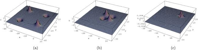
Figure 1. (a) Four-dromion structure of equation ( |
Example 2: There are some types of ring-type coherent structures that are not equal to zero identically at some closed curves and decay exponentially apart from the closed curves. By restricting the functions F, G as some summation forms of the exponential functions
$\begin{eqnarray}\begin{array}{l}F=\exp \left(-\displaystyle \frac{{\left(x-5t\right)}^{2}}{10}+6\right)\\ +\,\exp \left(-\displaystyle \frac{{\left(x+5t\right)}^{2}}{9}+2\right)+\exp \left(x+11t+1\right),\\ G=\exp \left(\displaystyle \frac{{y}^{2}}{10}-6\right),\end{array}\end{eqnarray}$
and a0 = 0, a1 = a2 = 1, a3 = 0, λ = 2, here we can obtain a ring-parabolic soliton structure (see figures 2(a)–(c)). With the increase of the time variable t, we can find that this structure has a fusion phenomenon, and finally tends to a parabolic soliton structure.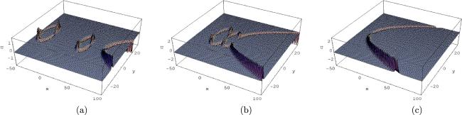
Figure 2. (a) Ring-parabolic soliton structure of equation ( |
4. Summary and discussions
We have considered the (2+1)-dimensional NNV-type system (1 ) by using the MLVS approach. In fact, this system (1 ) and the (2+1)-dimensional SS system (10 ) (or equation (8 )) are also first proposed by us. Starting from an auto-Bäcklund transformation and taking the MLVS ansatz f = F(x, t) + G(y, t) and seed solution {0, v0(x, t), w0(y, t)}, we can obtain much more general exact solutions of equation (1 ).
We can see that the (2+1)-dimensional NNV-type system (1 ) possesses some special types of coherent structures for the physical field u ≡ u(x, y, t) rather than the potentials v ≡ v(x, y, t) and w ≡ w(x, y, t). From expression equation (11 ), we know that equation (1 ) has an abundant coherent structure thanks to the arbitrariness of the functions of F(x, t) and G(y, t). Although the construction of (2+1)-dimensional coherent structures is more difficult than that of the (1+1)-dimensional case, new coherent structures represented by figures 1(a)–(c) and 2(a)–(c) for the physical quantity u are obtained.
The MLVS approach can be considered as a nonlinear extension of the variable separation approach in linear equations. We hope that the MLVS approach may be used for other multi-dimensional integrable (and/or even non-integrable) NLEEs [27–29]. The more about the physical properties of multi-dimensional coherent structures obtained by the MLVS approach is worthy of studying further.