


1. Introduction
Neurons play a crucial role in signal transmission and processing in organisms, and this has attracted widespread attention [1–5]. The biological nervous system contains hundreds of millions of glial cells and neurons, which develop and form in different functional regions. Nonlinear phenomena play a very important role in achieving corresponding biophysical functions under stimuli, thereby driving the body to make appropriate responses and stress activities, such as heartbeat, breathing, hearing, smelling, etc [6, 7]. The FithzHugh–Nagumo (FHN) model is widely used to describe the relationship between neuronal membrane potential and afferent stimuli, which can reproduce various firing modes of neurons, such as bursting, spiking, periodic and chaotic firings [8–11]. As a coupled oscillation system, its dynamic behavior can be effectively controlled through external stimuli, where sensors can be used to perceive external information [12–14]. When the input stimulus exceeds the threshold, the FHN model exhibits excitation oscillation properties, but when the input stimulus does not exceed the threshold, the FHN model is in a non-excitation state.
Considering the distinct physical properties of some functional electrical components, the neural circuits are improved to enhance their biophysical functions by incorporating specific electric components into circuits, such as piezoelectric ceramic, phototube, thermistor, etc. When the visual system is stimulated by external light signals, the nerves are activated and fire in different modes. Based on the characteristics of the phototube, the biophysical process of visual neurons can be simulated by introducing it into the FHN neuron circuit [15–17]. Temperature has a significant impact on the excitability of neurons [18–20]. When a thermistor is embedded in the neuron circuit, a thermistor neuron model can be obtained in which the firing modes and patterns are dependent on temperature [21]. Piezoelectric ceramic can be connected into a FHN neural circuit to obtain an improved functional neural circuit, which can be used to capture and encode external acoustic signals and produce various firing modes [22]. A phototube and a thermistor incorporated into different branches of the FHN neural circuit can develop a functional neuron that is controlled synchronously by external temperature and illumination [23, 24]. Josephson junction coupled neural circuits can detect the impact of external magnetic fields on neural electrical activity [25]. The memristor can be used for coupling between neural circuits to obtain memristor synapses, which is helpful to understand the occurrence of sudden heart disorders and heart failure subjected to electromagnetic radiation [26–29].
The nose can sense the gases in the environment that induce a sense of smell. The initial events in olfactory perception occur in olfactory sensory neurons in the nose. The olfactory sensory neuron is a bipolar nerve cell, in which thin cilia protrude into the layer of mucus that coats the epithelium. The cilia of the olfactory neuron are specialized for odor detection. They have specific receptors for odorants as well as the transduction machinery needed to amplify sensory signals and generate action potentials in the neuron's axon. When the gas signal is captured by the cilia in the nose, the pulse is transmitted to an olfactory neuron [30, 31]. Damage or loss of cilia can lead to odor impairment. For example, after the COVID-19 virus invades the human body, it can lead to an abnormal immune response, continuously damaging olfactory neurons, leading to weakened or even disappearing olfactory function [32, 33].
In order to discriminate it, an odorant must cause a distinct signal to be transmitted from the nose to the brain. That is to say, in the olfactory process, the first step is to convert external gas signals into electrical signals through physical and chemical reactions. When the olfactory sensory neuron binds to specific odorant receptors, a cascade of signal transduction events is initiated, and the ion channel will be activated. Then the external current will be injected into the olfactory neuron cells, causing changes in cell membrane potential. This process is similar to the working principle of field-effect transistors (FETs) [34]. Therefore, in this paper, both an FET and a gas sensor are embedded into the FHN neural circuit to develop an olfactory functional neural circuit. Herein, a gas sensor can be used to convert external gas concentration into the gate voltage of the FET, and control the continuity and disconnection between the drain and source electrodes. That is to say, the current injected into the FHN neural circuit can be controlled, thereby changing the firing states of the neural circuit. Furthermore, the gate voltage, threshold voltage and activation coefficient of the FET in this functional neural circuit can be used to study the effects of gas concentration, gas species and neuronal activity, respectively. It is meaningful for the preparation of artificial olfactory devices to assist and repair in the event of loss of and damage to olfactory function.
2. Model and scheme
Gas sensors are functional electronic components that can capture external gas signals to generate electric signals. FETs are commonly used as electronic switches. When a gas sensor and an FET are coupled into a simple FHN neural circuit, external gas signals can be perceived, and a gas-sensitive neural circuit is proposed, as shown in figure 1. Herein, ${i}_{{\rm{C}}}$ is the current from the linear capacitor, ${i}_{{\rm{L}}}$ is the current from the linear inductor, ${i}_{\mathrm{NR}}$ is the current from the nonlinear resistor, ${i}_{{\rm{D}}}$ is the source-drain current from the FET, ${U}_{{\rm{s}}}$ is the amplitude of the alternating voltage source, and $f$ is the frequency of the alternating voltage source.
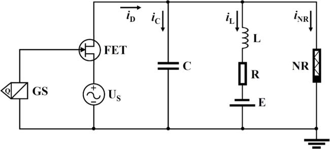
Figure 1. Schematic diagram of a gas-sensitive neural circuit incorporated within a gas sensor and an FET. GS represents the gas sensor, C is a linear capacitor, L is a linear inductor, R is a linear resistor, E is a constant voltage source, US is an alternating voltage source, and NR is a nonlinear resistor. Gas sensor is considered a voltage source. |
According to Kirchhoff's law, the circuit equation in figure 1 can be defined as:
$\begin{eqnarray}\left\{\begin{array}{l}C\displaystyle \frac{{\rm{d}}V}{{\rm{d}}t}={i}_{{\rm{D}}}-{i}_{{\rm{L}}}-{i}_{\mathrm{NR}}\\ L\displaystyle \frac{{\rm{d}}{i}_{{\rm{L}}}}{{\rm{d}}t}=V-R{i}_{{\rm{L}}}+E\end{array}\right.,\end{eqnarray}$
where $C$ is the capacitance of the linear capacitor, $L$ is the inductance of the linear inductor, $R$ is the resistance of the linear resistor, $E$ is the output voltage of the constant voltage source and $V$ is the applied voltage on the linear capacitor. The first equation is derived from Kirchhoff's current law, which states that the current flowing into the capacitor is equal to the current in the FET minus the current in the inductor and the current in the nonlinear resistor. The second equation is derived from Kirchhoff's voltage law, which represents the total voltage drop on the circuit composed of the linear inductor, linear capacitor and linear resistor, and the constant voltage source is zero.When a specific gas is received by the gas sensor, it can cause a potential in the sensor, and the potential voltage is related to the external gas concentration. The voltage in the gas sensor usually increases with higher gas concentration. Herein, a gas sensor is connected to the gate of the FET. ${V}_{{\rm{G}}}$ is the gate voltage, ${V}_{{\rm{T}}}$ is the threshold voltage and ${V}_{{\rm{D}}}$ is the source-drain voltage of the FET. As shown in figure 1, the voltage generated in the gas sensor is the gate voltage. When the gate voltage is less than the threshold voltage, there will be blockage between the source and drain, and the source-drain current ${i}_{{\rm{D}}}=0.$ When the gate voltage is greater than the threshold voltage, there will be conduction between the source and drain, and source-drain current ${i}_{{\rm{D}}}$ can be injected into the FHN neuron circuit through the FET.
The source-drain current ${i}_{{\rm{D}}}$ is defined as:
$\begin{eqnarray}\left\{\begin{array}{l}{i}_{{\rm{D}}}=\beta \left[\left({V}_{{\rm{G}}}-{V}_{{\rm{T}}}\right){V}_{{\rm{D}}}-\displaystyle \frac{1}{2}{V}_{{\rm{D}}}^{2}\right]\,0\lt {V}_{{\rm{D}}}\leqslant \left({V}_{{\rm{G}}}-{V}_{{\rm{T}}}\right)\\ {i}_{{\rm{D}}}=\displaystyle \frac{1}{2}\beta {\left({V}_{{\rm{G}}}-{V}_{{\rm{T}}}\right)}^{2}\,{V}_{{\rm{D}}}\gt \left({V}_{{\rm{G}}}-{V}_{{\rm{T}}}\right)\end{array}\right.,\end{eqnarray}$
where $\beta =\tfrac{{\mu }_{n}{C}_{{\rm{i}}}W}{L}$ is determined by the materials and structures of the FET, ${\mu }_{n}$ is the electron mobility in the channel, ${C}_{{\rm{i}}}$ is the capacitance per unit area of the insulation layer, $W$ and $L$ are the length and width of the gate of the FET, respectively.Some viruses or bacteria will destroy olfactory neurons after invading organisms, which will cause the olfactory function to be weakened or even disappear. Therefore, in the gas sensing neural circuit, the activation coefficient parameter η that characterizes the average activity of olfactory neurons is employed to adjust the source-drain current ID across the FET. The range of the parameter $\eta $ is usually from 0–1. Therefore, equation (3 ) is modified as:
$\begin{eqnarray}\left\{\begin{array}{l}{i}_{{\rm{D}}}=\eta \beta \left[\left({V}_{{\rm{G}}}-{V}_{{\rm{T}}}\right){V}_{{\rm{D}}}-\displaystyle \frac{1}{2}{V}_{{\rm{D}}}^{2}\right]\,0\lt {V}_{{\rm{D}}}\leqslant \left({V}_{{\rm{G}}}-{V}_{{\rm{T}}}\right)\\ {i}_{{\rm{D}}}=\displaystyle \frac{1}{2}\eta \beta {\left({V}_{{\rm{G}}}-{V}_{{\rm{T}}}\right)}^{2}\,{V}_{{\rm{D}}}\gt \left({V}_{{\rm{G}}}-{V}_{{\rm{T}}}\right)\end{array}.\right.\end{eqnarray}$
In addition, ${i}_{\mathrm{NR}}$ is often approximated by [22],
$\begin{eqnarray}{i}_{\mathrm{NR}}=-\displaystyle \frac{1}{\rho }\left(V-\displaystyle \frac{1}{3}\displaystyle \frac{{V}^{3}}{{V}_{0}^{2}}\right)\,,\end{eqnarray}$
where $\rho $ is the normalized resistance, while $V$ and ${V}_{0}$ denote the applied and cutoff voltages of the nonlinear resistor, respectively.Without loss of generality, the system needs standard scale transformation of the variables and intrinsic parameters as:
$\begin{eqnarray}\begin{array}{c}x=\displaystyle \frac{V}{{V}_{0}},\,y=\displaystyle \frac{\rho {i}_{L}}{{V}_{0}},\,\tau =\displaystyle \frac{t}{\rho C},\,a=\displaystyle \frac{E}{{V}_{0}},\,b=\displaystyle \frac{R}{\rho },\,\\ c=\displaystyle \frac{{\rho }^{2}C}{L},\,{u}_{{\rm{s}}}=\displaystyle \frac{{U}_{{\rm{s}}}}{{V}_{0}},\,\nu =\rho Cf,\,{I}_{{\rm{D}}}=\displaystyle \frac{\rho {i}_{{\rm{D}}}}{{V}_{0}},\\ \,{x}_{{\rm{T}}}=\displaystyle \frac{{V}_{{\rm{T}}}}{{V}_{0}}\,,\,{x}_{{\rm{G}}}=\displaystyle \frac{{V}_{{\rm{G}}}}{{V}_{0}},\,{x}_{{\rm{D}}}=\displaystyle \frac{{V}_{{\rm{D}}}}{{V}_{0}},\,{x}_{T}=\displaystyle \frac{{V}_{{\rm{T}}}}{{V}_{0}},\,K=\rho {V}_{0}\beta \,.\end{array}\end{eqnarray}$
Therefore, the gas-sensitive neural circuit (1) can be dimensionless as:
$\begin{eqnarray}\left\{\begin{array}{l}\displaystyle \frac{{\rm{d}}x}{{\rm{d}}\tau }=x-y-\displaystyle \frac{1}{3}{x}^{3}+{I}_{{\rm{D}}}\\ \displaystyle \frac{{\rm{d}}y}{{\rm{d}}\tau }=c\left(x-by+a\right)\end{array}\right.,\end{eqnarray}$
where ${I}_{{\rm{D}}}$ is the dimensionless source-drain current of the FET as: $\begin{eqnarray}\left\{\begin{array}{l}{I}_{{\rm{D}}}=\eta K\left[\left({x}_{{\rm{G}}}-{x}_{{\rm{T}}}\right){x}_{{\rm{D}}}-\displaystyle \frac{1}{2}{x}_{{\rm{D}}}^{2}\right]\,0\lt {x}_{{\rm{D}}}\leqslant \left({x}_{{\rm{G}}}-{x}_{{\rm{T}}}\right)\\ {I}_{{\rm{D}}}=\displaystyle \frac{1}{2}\eta K{\left({x}_{{\rm{G}}}-{x}_{{\rm{T}}}\right)}^{2}\,{x}_{{\rm{D}}}\gt \left({x}_{{\rm{G}}}-{x}_{{\rm{T}}}\right)\end{array}\right..\end{eqnarray}$
In addition, ${x}_{{\rm{D}}}$ can be obtained according to the total voltage drop in the branch of the FET and alternating voltage source as: $\begin{eqnarray}{x}_{{\rm{D}}}={u}_{{\rm{s}}}\,\cos \left(2\pi \nu \tau \right)-x\,.\end{eqnarray}$
The typical electrical characteristics of an ideal FET are shown in figure 2. Herein, we select $K=1$ and ${x}_{{\rm{T}}}=1.$ Figure 2(a) shows the relationship between ${I}_{{\rm{D}}}$ and ${x}_{{\rm{D}}}$ with different ${x}_{{\rm{G}}},$ which is commonly referred to as the output characteristic that shows the volt-ampere characteristic between the FET source and drain electrodes. Figure 2(b) shows the relationship between ${I}_{{\rm{D}}}$ and ${x}_{{\rm{G}}}$ with different ${x}_{{\rm{D}}},$ which is commonly referred to as the transfer characteristic that reveals the gain effect on the current.
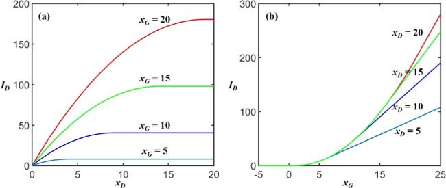
Figure 2. Typical electrical characteristics of an ideal FET with $K=1,$ $\eta =1$ and ${x}_{{\rm{T}}}=1$. |
The fixed point analysis of system (6) is shown in figure 3. The parameters are taken as $a=0.7,$ $b=0.8,$ $c=0.1,$ ${u}_{{\rm{s}}}=1,$ $K=1,$ ${x}_{{\rm{G}}}=2,$ ${x}_{{\rm{T}}}=1$ and $\eta =1.$ The red curve is $x$ nullcline, that is $\dot{x}=x-y-\tfrac{1}{3}{x}^{3}+{I}_{{\rm{D}}}=0.$ The green curve is $y$ nullcline, that is $\dot{y}=c\left(x-by+a\right)=0.$ The intersection of the green and red curves is the fixed point of the system (6). In addition, the black dashed curve is a reference nullcline of the original FHN model, that is $x-y-\tfrac{1}{3}{x}^{3}=0.$ Compared to the original FHN model, the $x$ nullcline of system (6) will translate and rotate in the phase plane, making the fixed point change along the $y$ nullcline.
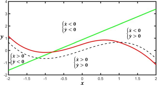
Figure 3. Fixed point analysis of system (6). Parameters are taken as $a=0.7,$ $b=0.8,$ $c=0.1,$ ${u}_{{\rm{s}}}=1,$ $K=1,$ ${x}_{{\rm{G}}}=2,$ ${x}_{{\rm{T}}}=1\,$and $\eta =1$ . |
In the case of biological neurons, energy is important in maintaining normal physiological function. Form the Helmholtz's theorem, the dimensionless Hamiltonian energy of system (6) is [4, 21],
$\begin{eqnarray}H=\displaystyle \frac{1}{2}{x}^{2}+\displaystyle \frac{1}{2c}{y}^{2}\,.\end{eqnarray}$
In addition, the average Hamiltonian energy can be effective to find firing mode dependence on the following: $\begin{eqnarray}H=\displaystyle \frac{1}{T}{\int }_{\tau =0}^{T}H\left(\tau \right){\rm{d}}\tau \,.\end{eqnarray}$
3. Numerical results and discussion
In this section, the fourth-order Runge–Kutta algorithm is applied to find numerical solutions for the neuron oscillators. The time step is ${\rm{\Delta }}\tau =0.01$ and the time span is about $1000$ time units. Neuron parameters are usually determined by experimental measurements and are then dimensionless by the standard scale transformation into a dynamic system. Thus, some invariant parameters are taken as $a=0.7,$ $b=0.8,$ $c=0.1,$ ${u}_{{\rm{s}}}=1,$ $K=1,$ and initial values are selected as ($0.1,$ $0.3$) [22].
To illustrate clearly, as presented in figures 4–7, an isolated functional neuron driven by different frequencies ($\nu $) is studied with the gate voltage ${x}_{{\rm{G}}}=2,$ the threshold voltage ${x}_{{\rm{T}}}=1$ and the activation coefficient $\eta =1.$ Due to the fact that system (6) is a bivariate system, complex chaotic phenomena generally do not occur. When a periodic excitation with appropriate frequency is applied, chaotic phenomena can be induced.
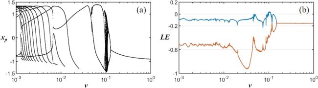
Figure 4. Bifurcation diagram and Lyapunov exponents of the gas-sensitive neural circuit with initial values ($0.1,$ $0.3$). Parameters are taken as $a=0.7,$ $b=0.8,$ $c=0.1,$ ${u}_{{\rm{s}}}=1,$ $K=1,$ ${x}_{{\rm{G}}}=2,$ ${x}_{{\rm{T}}}=1$ and $\eta =1.$ ${x}_{{\rm{p}}}$ is the peak value of signal $x$ and LE is the Lyapunov exponent. |
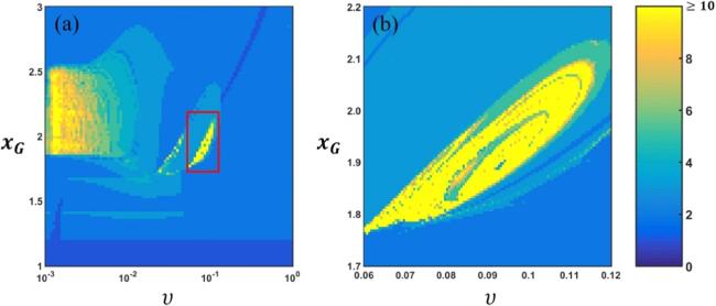
Figure 5. Dual parameter bifurcation diagram with gate voltage and frequency. Parameters are taken as $a=0.7,$ $b=0.8,$ $c=0.1,$ ${u}_{{\rm{s}}}=1,$ $K=1,$ ${x}_{{\rm{T}}}=1,$ $\eta =1$ and initial values ($0.1,$ $0.3$). Each color represents the number of peaks with different values. (a) Dual parameter bifurcation diagram, (b) the local enlarged drawing of the area enclosed by the red box. |
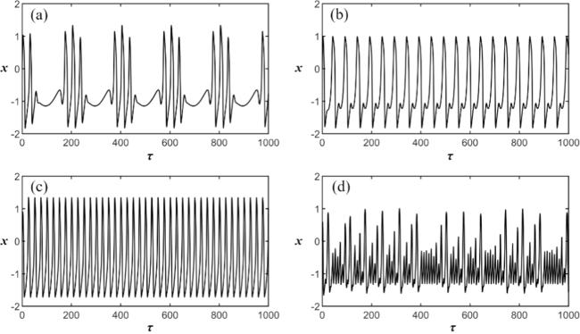
Figure 6. Time evolution of signal x by applying different frequencies to the alternating voltage source. Parameters are $a=0.7,$ $b=0.8,$ $c=0.1,$ ${u}_{{\rm{s}}}=1,$ $K=1,$ ${x}_{{\rm{G}}}=2,$ ${x}_{T}=1,$ $\eta =1,$ and initial values ($0.1,$ $0.3$). (a) Bursting mode with $\nu =0.005,$ (b) spiking mode with $\nu =0.02,$ (c) periodic firing mode with $\nu =0.04\,$and (d) chaotic mode with $\nu =0.1$. |
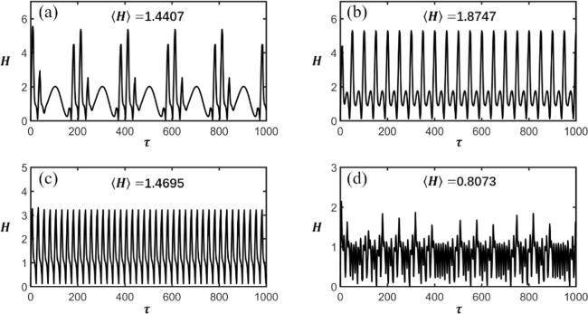
Figure 7. Time evolution of Hamiltonian energy with different frequencies. Parameters are $a=0.7,$ $b=0.8,$ $c=0.1,$ ${u}_{{\rm{s}}}=1,$ $K=1,$ ${x}_{{\rm{G}}}=2,$ ${x}_{{\rm{T}}}=1,$ $\eta =1$ and initial values ($0.1,$ $0.3$). (a) $\nu =0.005,$ (b) $\nu =0.02,$ (c) $\nu =0.04$ and (d) $\nu =0.1$. |
As shown in figure 4, the bifurcation analysis and the Lyapunov exponent analysis with different frequencies indicate that this circuit has rich dynamic behavior. The dual parameter bifurcation diagram with gate voltage (${x}_{{\rm{G}}}$) and frequency ($\nu $) is shown in figure 5. In the dual parameter bifurcation diagram, not only is the bifurcation of a single parameter presented, but also the rich dynamic behavior exhibited by system (6) when two parameters change simultaneously can be revealed. From bottom to top, the system transitions from the quiescent state (a single value) to a multi-peak firing state, followed by bursting or chaotic firing (by different excitation frequencies), and finally reaches a single-peak periodic firing, at which the system enters a saturation state. From left to right, the system transitions from bursting firing to single-peak or multi-peak firing state, followed by chaotic firing (by appropriate gate voltage), and finally reaches a single-peak periodic firing mode. The chaotic firing can occur approximately in the area around the frequency $\nu \unicode{x0007E}0.1$ and the gate voltage ${x}_{{\rm{G}}}\unicode{x0007E}2.$ That is to say, the appearance of chaos in this functional neuron depends on the appropriate selection of the double bifurcation parameters.
As shown in figure 6, it is demonstrated that the firing modes can be controlled to present bursting, spiking, periodic firing and then chaotic mode when the frequency is carefully selected. Figure 7 shows the time evolution of Hamiltonian energy with different frequencies. It can illustrate that the chaotic mode has a lower energy level while the bursting, spiking and periodic firing mode have higher energy levels. In addition, when the frequency is fixed, it is effective to regulate the firing state of neural activity by appropriately selecting external stimuli, such as gate voltage (${x}_{{\rm{G}}}$), threshold voltage (${x}_{{\rm{T}}}$) and activation coefficient ($\eta $).
3.1. The bursting mode
The response to external stimuli of the gas-sensitive neural circuit in the bursting mode is shown in figures 8–10. The fixed parameters are $a=0.7,$ $b=0.8,$ $c=0.1,$ ${u}_{{\rm{s}}}=1,$ $K=1,$ $v=0.005$ and initial values ($0.1,$ $0.3$). The results indicate that changing the gate and threshold voltages, and activation coefficient of the FET can effectively regulate the firing states of this circuit in bursting mode.
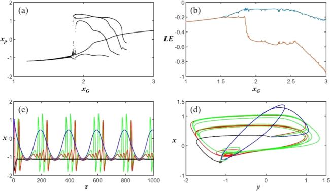
Figure 8. State in the bursting mode with different gate voltages. Fixed parameters ${x}_{{\rm{T}}}=1$ and $\eta =1.$ (a) Bifurcation diagram, (b) Lyapunov exponent, (c) time evolution of signal $x$ and (d) attractors. Black color represents ${x}_{{\rm{G}}}=1.5,$ red color represents ${x}_{{\rm{G}}}=1.85,$ green color represents ${x}_{{\rm{G}}}=2$ and blue color represents ${x}_{{\rm{G}}}=3$. |
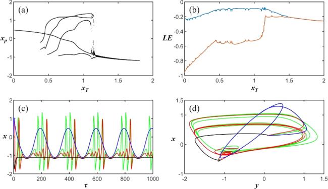
Figure 9. State in the bursting mode with different threshold voltages. Fixed parameters ${x}_{{\rm{G}}}=2$ and $\eta =1.$ (a) Bifurcation diagram, (b) Lyapunov exponent, (c) time evolution of signal $x$ and (d) attractors. Blue color represents ${x}_{{\rm{T}}}=0,$ green color represents ${x}_{{\rm{T}}}=1,$ red color represents ${x}_{{\rm{T}}}=1.15$ and black color represents ${x}_{{\rm{T}}}=1.5$. |
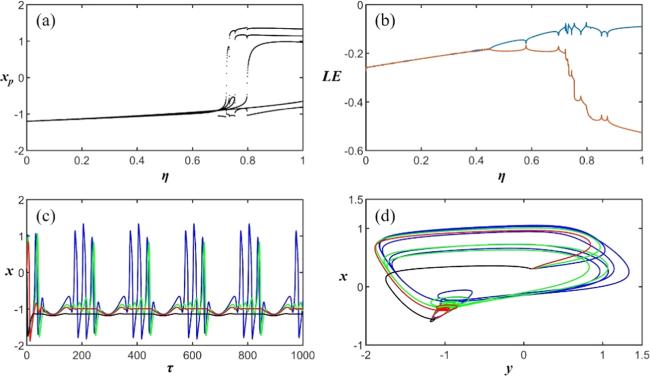
Figure 10. State in the bursting mode with different activation coefficients. Fixed parameters ${x}_{{\rm{T}}}=1$ and ${x}_{{\rm{G}}}=2.$ (a) Bifurcation diagram, (b) Lyapunov exponent, (c) time evolution of signal $x$ and (d) attractors. Black color represents $\eta =0.2,$ red color represents $\eta =0.6,$ green color represents $\eta =0.73$ and blue color represents $\eta =1$. |
For olfactory neurons, higher concentrations of odorant stimulate a larger number of neuronal cilia and cells. This may explain why odorants presented to human subjects at different concentrations can be perceived as being different. Therefore, it is considered that higher external gas concentrations generate a higher voltage on the gas sensor, resulting in an increase in the gate voltage of the FET. That is to say, as shown in figure 8, changing the external gas concentration generates different gate voltages to achieve the state variation of a gas-sensitive neural circuit. When the gate voltage is low (e.g. ${x}_{{\rm{G}}}=1.5$), the injected current does not exceed the threshold of FHN, and the circuit is in a quasi-quiescent state (as shown in black). As the gate voltage increases (e.g. ${x}_{{\rm{G}}}=1.85$), the injected current just reaches the threshold, and thus the circuit is in the quasi-bursting state (as shown in red). When the gate voltage further increases (e.g. ${x}_{{\rm{G}}}=2$), the injected current exceeds the threshold of the FHN circuit, and the circuit achieves the bursting state (as shown in green). While the gate voltage is high enough (e.g. ${x}_{{\rm{G}}}=3$), the injected current exhibits strong oscillation in the FHN circuit, causing the circuit to be in the saturated periodic firing state (as shown in blue).
In addition, different odorants stimulate different olfactory sensory neurons. This is accomplished primarily by the differing sensitivities of individual olfactory sensory neurons to different odorants. Meanwhile, the sensitivity of FETs can usually be distinguished by their threshold voltages. Without loss of generality, the lower the threshold voltage, the more sensitive the FET is, and the easier it is to conduct. Therefore, it is considered that the external gas species can also affect the gas-sensitive neural circuit via the threshold voltage of the FET. As shown in figure 9, changing the external gas species can induce different threshold voltages to achieve the state variation of the gas-sensitive neural circuit. When the threshold voltage is low (e.g. ${x}_{{\rm{T}}}=0$), the FET is easy to conduct, and the current injected into the FHN circuit is large enough to exhibit the circuit in a saturated periodic firing state (as shown in blue). As the threshold voltage increases (e.g. ${x}_{{\rm{T}}}=1$), the injected current drops to an appropriate range, and the circuit achieves the bursting state (as shown in green). When the threshold voltage continues to increase (e.g. ${x}_{{\rm{T}}}=1.15$), the injected current will decrease to near the threshold, resulting in the circuit being in a quasi-bursting state (as shown in red). When the threshold voltage further increases (e.g. ${x}_{{\rm{T}}}=1.5$), the injected current signal does not exceed the threshold. Thus, the circuit is in the quasi-quiescent state (as shown in black).
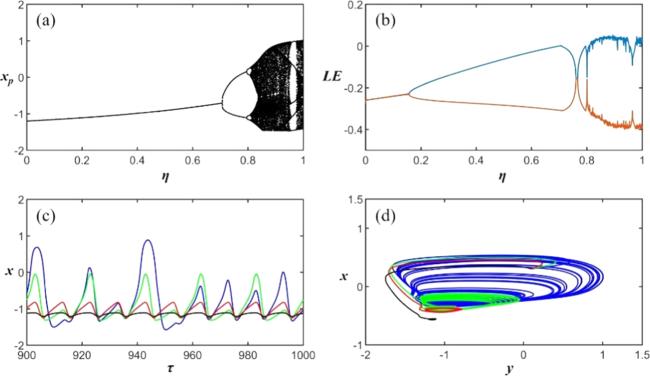
Furthermore, in diseases such as Parkinson's disease and the COVID-19 virus, inactivation of nerve cells can lead to a decrease in activity of neuron cilia and nerve cells, even apoptosis of neuron cilia and nerve cells. Therefore, it is considered that diseases and other factors can also affect the gas-sensitive neural circuit via the activation coefficient ($\eta $) within the range from $0$–$1.$ As shown in figure 10, the activation coefficient can regulate the activity states of the gas-sensitive neural circuit. When $\eta $ is low (e.g. $\eta =0.2$ and $\eta =0.6$), the injected current does not exceed the threshold of the FHN, and the circuit is in the quasi-quiescent state (as shown in black and red). As $\eta $ increases (e.g. $\eta =0.73$), the injected current significantly affects it to reach the threshold, and the circuit is in the quasi-bursting state (as shown in green). When $\eta $ is high enough (e.g. $\eta =1$), the injected current exceeds the threshold, and the circuit achieves the bursting state (as shown in blue).
3.2. The spiking mode
The response to external stimuli of the gas-sensitive neural circuit in the spiking mode is shown in figures 11–13. The fixed parameters are $a=0.7,$ $b=0.8,$ $c=0.1,$ ${u}_{{\rm{s}}}=1,$ $K=1,$ $v=0.02$ and initial values ($0.1,$ $0.3$).
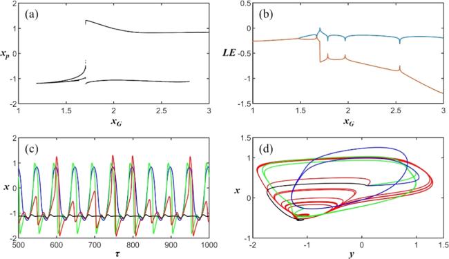
Figure 11. State in the spiking mode with different gate voltages. Fixed parameters ${x}_{{\rm{T}}}=1$ and $\eta =1.$ (a) Bifurcation diagram, (b) Lyapunov exponent, (c) time evolution of signal $x$ and (d) attractors. Black color represents ${x}_{{\rm{G}}}=1.5,$ red color represents ${x}_{{\rm{G}}}=1.704,$ green color represents ${x}_{{\rm{G}}}=2$ and blue color represents ${x}_{{\rm{G}}}=3$. |
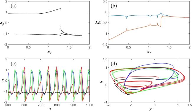
Figure 12. State in the spiking mode with different threshold voltages. Fixed parameters ${x}_{{\rm{G}}}=2$ and $\eta =1.$ (a) Bifurcation diagram, (b) Lyapunov exponent, (c) time evolution of signal $x$ and (d) attractors. Blue color represents ${x}_{{\rm{T}}}=0,$ green color represents ${x}_{{\rm{T}}}=1,$ red color represents ${x}_{{\rm{T}}}=1.296$ and black color represents ${x}_{{\rm{T}}}=1.5$. |
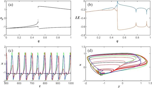
Figure 13. State in the spiking mode with different activation coefficients. Fixed parameters ${x}_{{\rm{T}}}=1$ and ${x}_{{\rm{G}}}=2.$ (a) Bifurcation diagram, (b) Lyapunov exponent, (c) time evolution of signal $x$ and (d) attractors. Black color represents $\eta =0.2,$ red color represents $\eta =0.4936,$ green color represents $\eta =0.6$ and blue color represents $\eta =1$. |
The influence of gate voltage on states of the gas-sensitive neural circuit in the spiking mode is shown in figure 11. When the gate voltage is low (e.g. ${x}_{{\rm{G}}}=1.5$), the current injected into the FHN circuit does not exceed the threshold, and the gas-sensitive neural circuit is in the quasi-quiescent state (as shown in black). As the gate voltage increases (e.g. ${x}_{{\rm{G}}}=1.704$ and ${x}_{{\rm{G}}}=2$), the injected current exceeds the threshold. However, unlike the bursting mode, the circuit will experience the chaotic mode (as shown in red) before achieving the spiking mode (as shown in green). When the gate voltage is high enough (e.g. ${x}_{{\rm{G}}}=3$), the injected current is sufficient to cause the circuit in the saturated periodic firing state (as shown in blue).
In addition, the influence of threshold voltage on the state of the gas-sensitive neural circuit in the spiking mode is shown in figure 12. When the threshold voltage is low (e.g. ${x}_{{\rm{T}}}=0$), the FET is easy to conduct, and the current injected into the FHN circuit is large enough to exhibit the circuit in a saturated periodic firing state (as shown in blue). As the threshold voltage increases (e.g. ${x}_{{\rm{T}}}=1$), the injected current exceeds the threshold, and the circuit is in the spiking state (as shown in green). When the threshold voltage further increases (e.g. ${x}_{{\rm{T}}}=1.296$ and ${x}_{{\rm{T}}}=1.5$), the injected current decreases, and the circuit will experience chaotic mode (as shown in red color) before entering the quasi-quiescent state (as shown in black).
Furthermore, the influence of the activation coefficient on the state of the gas-sensitive neural circuit in the spiking mode is shown in figure 13. When $\eta $ is low (e.g. $\eta =0.2$), the current injected into the FHN circuit does not exceed the threshold, and the circuit is in the quasi-quiescent state (as shown in black). As $\eta $ increases (e.g. $\eta =0.4936$), the injected current will reach the threshold, and the circuit will be in the chaotic mode (as shown in red). When $\eta $ continues growing (e.g. $\eta =0.6$ and $\eta =1$), the injected current exceeds the threshold, and the circuit will enter the spiking mode (as shown in green and blue).
3.3. The periodic firing mode
The response to external stimuli of the gas-sensitive neural circuit in the periodic firing mode is shown in figures 14–16. The fixed parameters are $a=0.7,$ $b=0.8,$ $c=0.1,$ ${u}_{{\rm{s}}}=1,$ $K=1,$ $v=0.04$ and initial values ($0.1,$ $0.3$).

Figure 14. State in the periodic firing mode with different gate voltages. Fixed parameters ${x}_{{\rm{T}}}=1$ and $\eta =1.$ (a) Bifurcation diagram, (b) Lyapunov exponent, (c) time evolution of signal $x$ and (d) attractors. Black color represents ${x}_{{\rm{G}}}=1.5,$ red color represents ${x}_{{\rm{G}}}=1.709,$ green color represents ${x}_{{\rm{G}}}=1.8$ and blue color represents ${x}_{{\rm{G}}}=2$. |
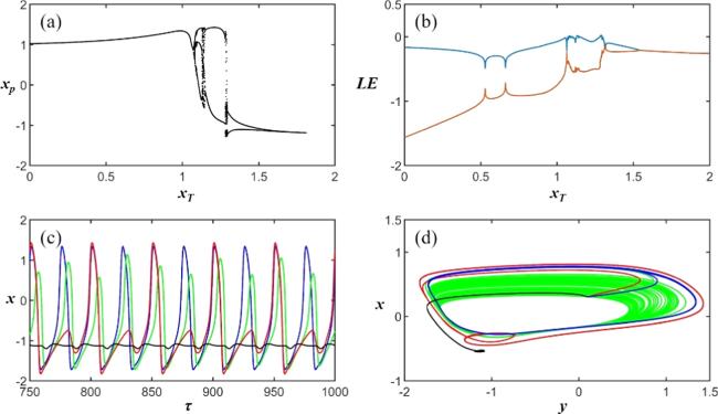
Figure 15. State in the periodic firing mode with different threshold voltages. Fixed parameters ${x}_{{\rm{G}}}=2$ and $\eta =1.$ (a) Bifurcation diagram, (b) Lyapunov exponent, (c) time evolution of signal $x$ and (d) attractors. Blue color represents ${x}_{{\rm{T}}}=1,$ green color represents ${x}_{{\rm{T}}}=1.081,$ red color represents ${x}_{{\rm{T}}}=1.2$ and black color represents ${x}_{{\rm{T}}}=1.5$. |
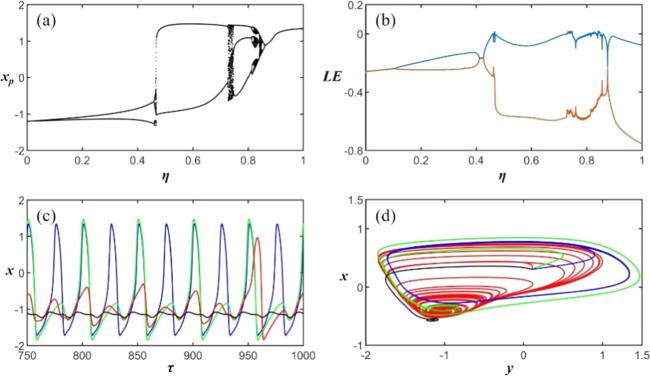
Figure 16. State in the periodic firing mode with different activation coefficients. Fixed parameters ${x}_{{\rm{T}}}=1$ and ${x}_{{\rm{G}}}=2.$ (a) Bifurcation diagram, (b) Lyapunov exponent, (c) time evolution of signal $x$ and (d) attractors. Black color represents $\eta =0.2,$ red color represents $\eta =0.467,$ green color represents $\eta =0.6$ and blue color represents $\eta =1$. |
The influence of gate voltage on the state of the gas-sensitive neural circuit in the periodic firing mode is shown in figure 14. When the gate voltage is low (e.g. ${x}_{{\rm{G}}}=1.5$), the circuit is in the quasi-quiescent state (as shown in black). As the gate voltage increases (e.g. ${x}_{{\rm{G}}}=1.709$ and ${x}_{{\rm{G}}}=1.8$), the states of the circuit will switch between chaotic and spiking modes (as shown in red and green). When the gate voltage continues growing (e.g. ${x}_{{\rm{G}}}=2$), the injected current is large enough to cause the circuit to be in the periodic firing state (as shown in blue).
In addition, the influence of threshold voltage on the state of the gas-sensitive neural circuit in the periodic firing mode is shown in figure 15. When the threshold voltage is low (e.g. ${x}_{{\rm{T}}}=1$), the current injected into the FHN circuit is large enough to exhibit the circuit in the periodic firing state (as shown in blue). As the threshold voltage increases (e.g. ${x}_{{\rm{T}}}=1.081$ and ${x}_{{\rm{T}}}=1.2$), the injected current gradually decreases to near the threshold, and the state of the circuit will switch between chaotic and spiking modes (as shown in green and red). When the threshold voltage further increases (e.g. ${x}_{{\rm{T}}}=1.5$), the injected current will be below the threshold, and the circuit will enter the quasi-quiescent state (as shown in black).
Furthermore, the influence of the activation coefficient on the state of the gas-sensitive neural circuit in the periodic firing mode is shown in figure 16. When $\eta $ is low (e.g. $\eta =0.2$), the circuit is in the quasi-quiescent state (as shown in black). As $\eta $ increases (e.g. $\eta =0.467$ and $\eta =0.6$), the state of the circuit will switch between chaotic and spiking modes (as shown in red and green color). When $\eta $ continues increasing (e.g. $\eta =1$), the circuit will enter the periodic firing mode (as shown in blue).
3.4. The chaotic mode
The response to external stimuli of the gas-sensitive neural circuit in chaotic mode is shown in figures 17–19. The fixed parameters are $a=0.7,$ $b=0.8,$ $c=0.1,$ ${u}_{{\rm{s}}}=1,$ $K=1,$ $v=0.1$ and initial values ($0.1,$ $0.3$).
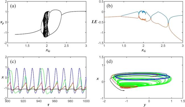
Figure 17. State in chaotic mode with different gate voltages. Fixed parameters ${x}_{{\rm{T}}}=1$ and $\eta =1.$ (a) Bifurcation diagram, (b) Lyapunov exponent, (c) time evolution of signal $x$ and (d) attractors. Black color represents ${x}_{{\rm{G}}}=1.5,$ red color represents ${x}_{{\rm{G}}}=1.85,$ green color represents ${x}_{{\rm{G}}}=2$ and blue color represents ${x}_{{\rm{G}}}=2.5$. |
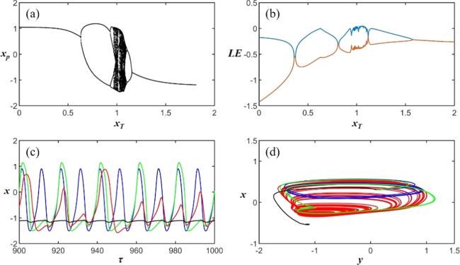
Figure 18. State in chaotic mode with different threshold voltages. Fixed parameters ${x}_{{\rm{G}}}=2$ and $\eta =1.$ (a) Bifurcation diagram, (b) Lyapunov exponent, (c) time evolution of signal $x$ and (d) attractors. Blue color represents ${x}_{{\rm{T}}}=0.5,$ green color represents ${x}_{{\rm{T}}}=0.85,$ red color represents ${x}_{{\rm{T}}}=1$ and black color represents ${x}_{{\rm{T}}}=1.5$. |
Figure 19. State in chaotic mode with different activation coefficients. Fixed parameters ${x}_{{\rm{T}}}=1$ and ${x}_{{\rm{G}}}=2.$ (a) Bifurcation diagram, (b) Lyapunov exponent, (c) time evolution of signal $x$ and (d) attractors. Black color represents $\eta =0.2,$ red color represents $\eta =0.6,$ green color represents $\eta =0.75$ and blue color represents $\eta =1$. |
The influence of gate voltage on the state of the gas-sensitive neural circuits in chaotic mode is shown in figure 17. When the gate voltage is low (e.g. ${x}_{{\rm{G}}}=1.5$), the injected current does not exceed the threshold, and the circuit is in the quasi-quiescent state (as shown in black). As the gate voltage increases (e.g. ${x}_{{\rm{G}}}=1.85$), the injected current will gradually reach the threshold, and the state of the circuit will be in the spiking mode (as shown in red color). As the gate voltage continues increasing (e.g. ${x}_{{\rm{G}}}=2$), the injected current exceeds the threshold, and the circuit will achieve a chaotic state (as shown in green). When the gate voltage continues growing (e.g. ${x}_{{\rm{G}}}=2.5$), the injected current is large enough to cause the circuit to go through the spiking state and then enter the periodic firing state (as shown in blue).
In addition, the influence of threshold voltage on the state of the gas-sensitive neural circuits in the chaotic mode is shown in figure 18. When the threshold voltage is low (e.g. ${x}_{{\rm{T}}}=0.5$), the current injected into the FHN circuit is large enough to exhibit the circuit in the periodic firing state (as shown in blue). As the threshold voltage increases (e.g. ${x}_{{\rm{T}}}=0.85$), the injected current gradually decreases to cause the circuit to enter the spiking state (as shown in green). When the threshold voltage further increases (e.g. ${x}_{{\rm{T}}}=1$), the state of the circuit will achieve chaotic mode (as shown in red). When the threshold voltage is much higher (e.g. ${x}_{{\rm{T}}}=1.5$), the injected current will be below the threshold, and the circuit will stay in the quasi-quiescent state (as shown in black).
Furthermore, the influence of the activation coefficient on the state of the gas-sensitive neural circuits in the chaotic mode is shown in figure 19. When $\eta $ is low (e.g. $\eta =0.2$ and $\eta =0.6$), the circuit stays in the quasi-quiescent state (as shown in black and red). As $\eta $ increases (e.g. $\eta =0.75$), the circuit will enter the spiking mode (as shown in green). While $\eta $ continues increasing (e.g. $\eta =1$), the circuit will achieve chaotic mode (as shown in blue).
4. Conclusion
In this paper, a functional neural circuit is designed by incorporating a gas sensor and an FET into a simple FHN neural circuit to sense external gas signals. By applying appropriate scale transformations to the circuit equations, a functional olfactory neuron model is obtained. The gas sensor is connected to the gate of the FET, which can change the gate voltage of the FET according to the gas concentration. When the gas concentration is low, the gate voltage is less than the threshold voltage of the FET. The FHN circuit cannot be excited, so the circuit is in a quasi-quiescent state, and the signal x is close to the resting potential. As the gas concentration increases, the gate voltage exceeds the threshold voltage of the FET. The FHN circuit can be effectively stimulated, and the circuit presents bursting, spiking, periodic and even chaotic firing patterns similar to those in biological neurons by carefully changing the frequency of the alternating voltage source. When the gas concentration is high enough, the system will reach saturation, and the injected current exhibits strong oscillations in the FHN circuit, causing the circuit to be in the saturated periodic firing state. In addition, analogous to the perceptual characteristics of olfactory neurons in real organisms, the stimuli of gas species and neuronal activity are presented as the threshold voltage and activation coefficient of the FET, respectively. The influence of threshold voltage and activation coefficient on states of the functional neural circuit are also studied. This shows that changing the external stimulus signals of the FET effectively regulates the firing states of circuit activities, even switching between different firing modes. We have studied individual neurons. However, the olfactory function requires the collective collaboration of a large number of neurons, and we will further study the olfactory neural networks. These results provide good guidance for the further application of intelligent sensors, the design of artificial olfactory devices and other coupled systems of real-life applications.
Generally, a capacitive variable is employed for estimating the changes of membrane potential and an inductive variable is employed for the channel current of calcium, potassium and sodium along the membrane channels. However, the physical properties of actual biological neurons are very complex. Considering that biological neurons have both inner and outer membranes, it is necessary to introduce a dual capacitance model to describe their potentials, and the medium between the two membranes is also worth studying. Meanwhile, using an inductor to estimate channel currents has limitations, which overlook the differences between ions and the effects of ion channel switching. Moreover, in the process of realizing the functions of biological neurons, phenomena such as heat, magnetism and light often occur simultaneously, which requires the combination of different functional devices to evaluate the combined impact of these effects. These issues need to be considered in future study in order to improve this gas sensing neural circuit.