


1. Introduction
Quantum teleportation was proposed by Bennett et al for more than 30 years [1, 2]. It is an amazing product of quantum entanglement that opens the door of quantum communication. This gives rise to many new methods of quantum information transmission, such as quantum remote state preparation (RSP) [3–5], quantum cloning [6–8], quantum information concentration [9, 10] and so on [11–13]. Quantum teleportation is also the main method of information transfer in entanglement distribution networks [14]. Important progress in quantum teleportation has been made both theoretically [15, 16] and experimentally [17, 18].
The idea of quantum RSP has many similarities to teleportation, such as the need to share entangled states to connect two communication parties [19–23]. The difference is that the sender in the RSP protocol only has the classical information of the transmitted qubit but does not possess the corresponding physical entity of the qubit. Therefore, when it is difficult to obtain the physical particles of qubits, RSP is a good alternative. RSP and its modifications have been widely investigated over the last 20 years [24–29].
In the quantum RSP process, classical information of the target state is usually assigned to one sender. If the sender is dishonest or negative, information leakage may occur. To improve communication security, scholars have proposed involving more parties in RSP, e.g. multiparty RSP [30] and joint remote state preparation (JRSP) [31]. In JRSP, the classical information of the state to be prepared is distributed to two or more senders. Senders must cooperate with each other to complete the quantum state preparation, thereby reducing the risk of information leakage [32–36]. JRSP has been investigated from many aspects, including the preparation of single, two, three and special multiqubits [37–43]; cluster states [44–47]; χ-square states [48]; and equatorial states [49–51].
However, most RSP and JRSP schemes focus on the transmission of information to one receiver, which does not satisfy the demand of multiple users. As an important method of information transmission in quantum networks, quantum multicast can satisfy the demand of synchronously sending different information to multiple receivers [52, 53]. In quantum multicast, if the information received by the receivers is the same, it is called quantum broadcasting. Xu et al introduced quantum cooperative multicast and proposed a scheme of cooperative multicast on butterfly network [54]. In 2018, Yu and Zhao investigated the broadcast and multicast problems of a single qubit based on the maximum entangled Bell state [55]. In 2019, Yu et al presented an RSP protocol of arbitrary two qubits with real coefficients, based on quantum multicast [56]. Subsequently, Zhao et al proposed quantum multicast scheme of arbitrary Greenberger–Horne–Zeilinger (GHZ)-class states based on RSP [57]. In 2022, Pan et al exhibited a two-pair quantum multicast on butterfly networks using network coding and extended it to k-pair [58]. Using partially entangled states as shared resources, Peng et al investigated the multicast of a special four-qubit complex coefficient cluster-type state based on RSP [59]. Recently, they proposed quantum multicast of an arbitrary two-qubit state using a nine-qubit entangled state [60].
Based on an analysis of the aforementioned studies, we found that there is no relevant research on the multicast of an arbitrary three-qubit state. Inspired by the idea in literature [57, 59, 60], we attempted to explore the multicast of any three-qubit state. In this study, using the maximally entangled GHZ states as shared channels and dividing the information of qubits into amplitude and phase groups, we complete the multicast schemes of arbitrary single- and two-qubit states. Based on the single- and two-qubit multicast method, we present a multicast scheme of three qubits. Corresponding quantum state tomography was performed on the IBM Quantum (IBMQ) platform to check the effectiveness of the schemes.
The remainder of this paper is organized as follows. In section 2 , we present theoretical multicast schemes for arbitrary single, two and three qubits. In section 3 , we present the experimental simulation results of the multicast scheme for specific states. In section 4 , we analyze the efficiency of our scheme and investigate the effect of noise. We conclude the paper in section 5 .
2. Theoretical protocols of quantum multicast
2.1. Theoretical multicast scheme of an arbitrary single-qubit state
In this subsection, we describe the concrete quantum multicast scheme of a single qubit based on JRSP.
In the scheme, two senders, named Alice1 and Alice2, and N receivers, named Bob1, Bob2, ⋯, BobN, are involved. There are N qubit states $| {\varphi }_{1}\rangle ={a}_{1}| 0\rangle +{b}_{1}{{\rm{e}}}^{{\rm{i}}{\theta }_{1}}| 1\rangle $, ⋯, $| {\varphi }_{N}\rangle ={a}_{N}| 0\rangle +{b}_{N}{{\rm{e}}}^{{\rm{i}}{\theta }_{N}}| 1\rangle $, where ai, bi and θi are real numbers satisfying the normalization condition ${a}_{i}^{2}+{b}_{i}^{2}=1$, where i = 1, 2, ⋯ , N. Information on N qubits is divided into two groups. The first sender, Alice1, holds all information of amplitudes ai and bi. The second sender, Alice2, possesses all information of phases θi. The two senders want the receiver Bobi to achieve the state $| {\varphi }_{i}\rangle ={a}_{i}| 0\rangle +{b}_{i}{{\rm{e}}}^{i{\theta }_{i}}| 1\rangle $ simultaneously at the end of the communication, without sending physical particles during the entire process.
To complete the task described previously, the senders and receivers should share N maximally entangled three-qubit GHZ states denoted by $| { \mathcal S }\rangle $ as follows:
$\begin{eqnarray}\begin{array}{l}| { \mathcal S }\rangle =| \mathrm{GHZ}{\rangle }^{\otimes N}\\ =\,\displaystyle \frac{1}{\sqrt{2}}{\left(| 000\rangle +| 111\rangle \right)}_{123}\otimes \cdots \\ \otimes \displaystyle \frac{1}{\sqrt{2}}{\left(| 000\rangle +| 111\rangle \right)}_{3N-\mathrm{2,3}N-\mathrm{1,3}N}.\end{array}\end{eqnarray}$
Each sender obtains one particle from each GHZ state. As a result, Alice1 and Alice2 each has N particles. Each Bobi holds one particle. Figure 1 clearly shows the distribution of particles in this scheme. In figure 1, the black dots represent qubits, and the black dots connected by green lines are in the GHZ state relationship. Qubits 1, 4, ... , 3N − 2 belong to Alice1; qubits 2, 5, ... , 3N − 1 belong to Alice2; and qubits 3, 6, ... , 3N belong to Bob1, Bob2, ... , BobN, respectively. In fact, it is not necessary to number the qubits. We only need to ensure that Alice1 and Alice2 each has N qubits, and each Bobi has one qubit. These are numbered here for easier calculations later. Based on the preceding assumptions and demands, the multicast of single qubits can be completed in three steps.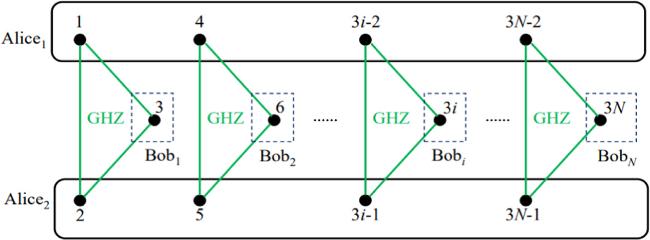
Figure 1. Distribution of shared qubits in the multicast scheme of single qubits. |
Step 1. Alice1 makes projective measurement {∣μi⟩} on her N particles based on the amplitude information. The measurement {∣μi⟩, where i = 0, 1, ⋯ , 2N − 1}, is constructed in the following way:
$\begin{eqnarray}\left(\begin{array}{c}| {\mu }_{0}\rangle \\ | {\mu }_{1}\rangle \\ \vdots \\ | {\mu }_{{2}^{N}-1}\rangle \end{array}\right)=\left(\underset{k=1}{\overset{N}{\bigotimes }}{\eta }_{k}\right)\left(\begin{array}{c}| 00\cdots 00\rangle \\ | 00\cdots 01\rangle \\ \vdots \\ | 11\cdots 11\rangle \end{array}\right),\end{eqnarray}$
where the 2 × 2 matrix ηk defined using the amplitude of ∣φk⟩ is $\begin{eqnarray}{\eta }_{k}=\left(\begin{array}{cc}{a}_{k} & {b}_{k}\\ -{b}_{k} & {a}_{k}\end{array}\right).\end{eqnarray}$
The binary expression of the measurement result of Alice1 is denoted as i1i2 ⋯ iN.Step 2. According to Alice1's measurement result i1i2 ⋯ iN (where the decimal representation is denoted as r), Alice2 makes projective measurement $\{| {\nu }_{i}^{r}\rangle \}$ on her N particles based on the phase information. The measurement basis is $\{| {\nu }_{i}^{r}\rangle ,i=0,\cdots ,\,{2}^{N}-1\}$, as follows:
$\begin{eqnarray}\left(\begin{array}{c}| {\nu }_{0}^{r}\rangle \\ | {\nu }_{1}^{r}\rangle \\ \vdots \\ | {\nu }_{{2}^{N}-1}^{r}\rangle \end{array}\right)=\left(\underset{k=1}{\overset{N}{\displaystyle \bigotimes }}({\zeta }_{k}{X}^{{i}_{k}})\right)\left(\begin{array}{c}| 00\cdots 00\rangle \\ | 00\cdots 01\rangle \\ \vdots \\ | 11\cdots 11\rangle \end{array}\right),\end{eqnarray}$
where the unitary operation ζk defined using the phase information of ∣φk⟩ is $\begin{eqnarray}{\zeta }_{k}=\displaystyle \frac{1}{\sqrt{2}}\left(\begin{array}{cc}1 & {{\rm{e}}}^{-{\rm{i}}{\theta }_{k}}\\ 1 & -{{\rm{e}}}^{-{\rm{i}}{\theta }_{k}}\end{array}\right).\end{eqnarray}$
The binary representation of the measurement result of Alice2 is denoted as j1j2 ⋯ jN.Step 3. Bob1, Bob2, ⋯, BobN perform recovery operation according to the measurement results of Alice1 and Alice2. Bobk executes recovery operation ${Z}^{{j}_{k}}{({ZX})}^{{i}_{k}}$ on his qubit, in which the Pauli operations are expressed as follows:
$\begin{eqnarray}X=\left(\begin{array}{cc}0 & 1\\ 1 & 0\end{array}\right),\quad Z=\left(\begin{array}{cc}1 & 0\\ 0 & -1\end{array}\right).\end{eqnarray}$
In the following, we explain the scheme using the case of three receivers, i.e. N = 3. Two senders, Alice1 and Alice2, and three receivers, Bob1, Bob2 and Bob3, share the composite of three GHZ states as follows:
$\begin{eqnarray}\begin{array}{l}| { \mathcal S }\rangle =\displaystyle \frac{1}{2\sqrt{2}}{\left(| 000\rangle +| 111\rangle \right)}_{123}\\ \quad \otimes {\left(| 000\rangle +| 111\rangle \right)}_{456}\otimes {\left(| 000\rangle +| 111\rangle \right)}_{789}.\end{array}\end{eqnarray}$
The initial system state can be rearranged as $\begin{eqnarray}\begin{array}{l}| { \mathcal S }\rangle =\displaystyle \frac{1}{2\sqrt{2}}\left(| 000{\rangle }^{\otimes 3}+| 001{\rangle }^{\otimes 3}+| 010{\rangle }^{\otimes 3}+| 011{\rangle }^{\otimes 3}\right.\\ \quad {\left.\quad +\,| 100{\rangle }^{\otimes 3}+| 101{\rangle }^{\otimes 3}+| 110{\rangle }^{\otimes 3}+| 111{\rangle }^{\otimes 3}\right)}_{\mathrm{147,258,369}}.\end{array}\end{eqnarray}$
Assuming that the measurement result of Alice1 is ∣μ6⟩, the corresponding binary representation is 110. In the case of three receivers, ∣μ6⟩ has the following form: $\begin{eqnarray}\begin{array}{l}| {\mu }_{6}\rangle ={b}_{1}{b}_{2}{a}_{3}| 000\rangle +{b}_{1}{b}_{2}{b}_{3}| 001\rangle \\ \,-{b}_{1}{a}_{2}{a}_{3}| 010\rangle -{b}_{1}{a}_{2}{b}_{3}| 011\rangle \\ -\,{a}_{1}{b}_{2}{a}_{3}| 100\rangle -{a}_{1}{b}_{2}{b}_{3}| 101\rangle \\ \,+{a}_{1}{a}_{2}{a}_{3}| 110\rangle +{a}_{1}{a}_{2}{b}_{3}| 111\rangle .\end{array}\end{eqnarray}$
The collapsed system state of Alice2, Bob1, Bob2 and Bob3 is $\begin{eqnarray}\begin{array}{l}{\left(-{b}_{1}| 00\rangle +{a}_{1}| 11\rangle \right)}_{23}\left(-{b}_{2}| 00\rangle \right.\\ {\left.\,+{a}_{2}| 11\rangle \right)}_{56}{\left({a}_{3}| 00\rangle +{b}_{3}| 11\rangle \right)}_{89}.\end{array}\end{eqnarray}$
According to the measurement result of Alice1, Alice2 performs projective measurements on qubits 2, 5 and 8, as follows: $\begin{eqnarray}\begin{array}{l}\left(\begin{array}{c}| {\nu }_{0}^{6}\rangle \\ | {\nu }_{1}^{6}\rangle \\ \vdots \\ | {\nu }_{7}^{6}\rangle \end{array}\right)=\displaystyle \frac{1}{2\sqrt{2}}\left(\begin{array}{cc}{{\rm{e}}}^{-{\rm{i}}{\theta }_{1}} & 1\\ -{{\rm{e}}}^{-{\rm{i}}{\theta }_{1}} & 1\end{array}\right)\otimes \left(\begin{array}{cc}{{\rm{e}}}^{-{\rm{i}}{\theta }_{2}} & 1\\ -{{\rm{e}}}^{-{\rm{i}}{\theta }_{2}} & 1\end{array}\right)\\ \,\otimes \,\left(\begin{array}{cc}1 & {{\rm{e}}}^{-{\rm{i}}{\theta }_{3}}\\ 1 & -{{\rm{e}}}^{-{\rm{i}}{\theta }_{3}}\end{array}\right)\left(\begin{array}{c}| 000\rangle \\ | 001\rangle \\ \vdots \\ | 111\rangle \end{array}\right).\end{array}\end{eqnarray}$
Assume that the measurement outcome of Alice2 is 101. That is, Alice2 measures qubits 2, 5 and 8 in $| {\nu }_{5}^{6}\rangle $, as follows: $\begin{eqnarray}\begin{array}{l}|{\nu }_{5}^{6}\rangle =\displaystyle \frac{1}{2\sqrt{2}}(-{{\rm{e}}}^{-{\rm{i}}{\theta }_{1}}|0\rangle +|1\rangle )\\ \,\times \,({{\rm{e}}}^{-{\rm{i}}{\theta }_{2}}|0\rangle +|1\rangle )(|0\rangle -{{\rm{e}}}^{-{\rm{i}}{\theta }_{3}}|1\rangle ).\end{array}\end{eqnarray}$
After the measurement of Alice1 and Alice2, the collapsed system state of Bob1, Bob2 and Bob3 is $\begin{eqnarray}\begin{array}{l}({b}_{1}{{\rm{e}}}^{{\rm{i}}{\theta }_{1}}| 0\rangle +{a}_{1}| 1\rangle )(-{b}_{2}{{\rm{e}}}^{{\rm{i}}{\theta }_{2}}| 0\rangle +{a}_{2}| 1\rangle )\\ \,\times \,({a}_{3}| 0\rangle -{b}_{3}{{\rm{e}}}^{{\rm{i}}{\theta }_{3}}| 1\rangle ).\end{array}\end{eqnarray}$
After receiving the measurement results of Alice1 and Alice2, Bob1, Bob2 and Bob3 perform X, ZX and Z operations on their particles, respectively. Finally, they obtain the desired state synchronously.Note that if we continue to introduce n − 1 auxiliary qubits in state ∣0⟩⨂(n−1) for each Bobk, and Bobk performs n − 1 CNOT gates with the auxiliary qubits as the target states, the n-qubit GHZ-type state ${a}_{k}| 00\cdots 0\rangle +{b}_{k}{{\rm{e}}}^{{\rm{i}}{\theta }_{k}}| 11\cdots 1\rangle $ could be obtained by Bobk simultaneously.
2.2. Theoretical multicast scheme of an arbitrary two-qubit state
In the two-qubit multicast scheme, there are also two senders and N receivers. The names in section 2.1 are carried over to this section. The two senders want the receiver, Bobi (where i = 1, 2, ⋯ , N), to receive the information of
$\begin{eqnarray}\begin{array}{l}| {\varphi }_{i}\rangle ={a}_{i}{{\rm{e}}}^{{\rm{i}}{\alpha }_{i}}| 00\rangle +{b}_{i}{{\rm{e}}}^{{\rm{i}}{\beta }_{i}}| 01\rangle \\ \quad +\,{c}_{i}{{\rm{e}}}^{{\rm{i}}{\gamma }_{i}}| 10\rangle +{d}_{i}{{\rm{e}}}^{{\rm{i}}{\delta }_{i}}| 11\rangle ,\end{array}\end{eqnarray}$
where the amplitude {ai, bi, ci, di} and phase {αi, βi, γi, δi} are real numbers. The amplitude coefficients satisfy the normalization condition ${a}_{i}^{2}+{b}_{i}^{2}+{c}_{i}^{2}+{d}_{i}^{2}=1$. The amplitude and phase information is distributed to Alice1 and Alice2, respectively.To complete the two-qubit state multicast, the whole initial system state shared among the senders and receivers is
$\begin{eqnarray}\begin{array}{l}| { \mathcal S }\rangle =| \mathrm{GHZ}{\rangle }^{\otimes 2N}\\ \quad =\,\displaystyle \frac{1}{\sqrt{2}}{\left(| 000\rangle +| 111\rangle \right)}_{123}\otimes \cdots \\ \otimes \displaystyle \frac{1}{\sqrt{2}}{\left(| 000\rangle +| 111\rangle \right)}_{6N-\mathrm{2,6}N-\mathrm{1,6}N}.\end{array}\end{eqnarray}$
Alice1 and Alice2 each has 2N particles of the shared states, whereas each Bobi possesses two particles. Particles 1, 4, 7, ⋯ , 6N − 2 are distributed to Alice1 and 2, 5, 8, ⋯ , 6N − 1 to Alice2. Bobi holds particles 6i − 3 and 6i. The distribution of qubits is illustrated in figure 2.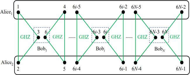
Figure 2. Distribution of shared qubits in the multicast scheme of two-qubit states. |
The two-qubit quantum multicast scheme consists of the following steps:
Step 1. Alice1 makes projective measurement {∣μi⟩, where i = 0, ⋯ , 22N − 1}, on her 2N qubits. The measurement is constructed as follows:
$\begin{eqnarray}\left(\begin{array}{c}| {\mu }_{0}\rangle \\ | {\mu }_{1}\rangle \\ \vdots \\ | {\mu }_{{2}^{2N}-1}\rangle \end{array}\right)=\left(\underset{k=1}{\overset{N}{\displaystyle \bigotimes }}{\eta }_{k}\right)\left(\begin{array}{c}| 00\ldots 00\rangle \\ | 00\ldots 01\rangle \\ \vdots \\ | 11\ldots 11\rangle \end{array}\right),\end{eqnarray}$
in which the two-qubit unitary operation ηk is $\begin{eqnarray}{\eta }_{k}=\left(\begin{array}{cccc}{a}_{k} & {b}_{k} & {c}_{k} & {d}_{k}\\ {b}_{k} & -{a}_{k} & {d}_{k} & -{c}_{k}\\ {c}_{k} & -{d}_{k} & -{a}_{k} & {b}_{k}\\ {d}_{k} & {c}_{k} & -{b}_{k} & -{a}_{k}\end{array}\right).\end{eqnarray}$
The measurement result of Alice1 is denoted by i1i2 ⋯ i2N, and the corresponding decimal expression is r.Step 2. According to Alice1's measurement result r (where the corresponding binary expression is i1i2 ⋯ i2N) and phase information, Alice2 performs projective measurement $\{| {\nu }_{i}^{r}\rangle ,i=0,\cdots ,\,{2}^{2N}-1\}$, as follows:
$\begin{eqnarray}\left(\begin{array}{c}| {\nu }_{0}^{r}\rangle \\ | {\nu }_{1}^{r}\rangle \\ \vdots \\ | {\nu }_{{2}^{2N}-1}^{r}\rangle \end{array}\right)=\left(\underset{k=1}{\overset{N}{\displaystyle \bigotimes }}{\zeta }_{k}({X}^{{i}_{2k-1}}\otimes {X}^{{i}_{2k}})\right)\left(\begin{array}{c}| 00\ldots 00\rangle \\ | 00\ldots 01\rangle \\ \vdots \\ | 11\ldots 11\rangle \end{array}\right),\end{eqnarray}$
where $\begin{eqnarray}{\zeta }_{k}=\displaystyle \frac{1}{2}\left(\begin{array}{cccc}{{\rm{e}}}^{-{\rm{i}}{\alpha }_{k}} & {{\rm{e}}}^{-{\rm{i}}{\beta }_{k}} & {{\rm{e}}}^{-{\rm{i}}{\gamma }_{k}} & {{\rm{e}}}^{-{\rm{i}}{\delta }_{k}}\\ {{\rm{e}}}^{-{\rm{i}}{\alpha }_{k}} & -{{\rm{e}}}^{-{\rm{i}}{\beta }_{k}} & {{\rm{e}}}^{-{\rm{i}}{\gamma }_{k}} & -{{\rm{e}}}^{-{\rm{i}}{\delta }_{k}}\\ {{\rm{e}}}^{-{\rm{i}}{\alpha }_{k}} & {{\rm{e}}}^{-{\rm{i}}{\beta }_{k}} & -{{\rm{e}}}^{-{\rm{i}}{\gamma }_{k}} & -{{\rm{e}}}^{-{\rm{i}}{\delta }_{k}}\\ {{\rm{e}}}^{-{\rm{i}}{\alpha }_{k}} & -{{\rm{e}}}^{-{\rm{i}}{\beta }_{k}} & -{{\rm{e}}}^{-{\rm{i}}{\gamma }_{k}} & {{\rm{e}}}^{-{\rm{i}}{\delta }_{k}}\end{array}\right).\end{eqnarray}$
Assume that the binary expression of the measurement result of Alice2 is j1j2 ⋯ j2N.Step 3. The receiver, Bobk, achieves the desired state by performing recovery operation:
$\begin{eqnarray}\begin{array}{l}{Z}_{6k-3}^{{j}_{2k-1}}{\left({Z}_{6k-3}{X}_{6k-3}\right)}^{{i}_{2k-1}}\\ \otimes {Z}_{6k}^{{j}_{2k}}{Z}_{6k}^{{i}_{2k-1}\oplus {i}_{2k}}{X}_{6k}^{{i}_{2k}},\end{array}\end{eqnarray}$
on qubits 6k − 3 and 6k (where k = 1, 2, ⋯ , N), where the symbol ⊕ represents the addition of module 2.To facilitate understanding, we illustrate the preceding scheme with an example of three recipients. When N = 3, the initial state of the system is20 ), the recovery operation of Bob1 is Z3X3 ⨂ Z6X6, Bob2 is Z9 and Bob3 is Z15X15, which achieve the desired states exactly.
$\begin{eqnarray}| { \mathcal S }\rangle =\displaystyle \frac{1}{{2}^{3}}{\left(| 000\rangle +| 111\rangle \right)}_{123}\otimes \cdots \otimes {\left(| 000\rangle +| 111\rangle \right)}_{\mathrm{16,17,18}}.\end{eqnarray}$
Assuming that the measurement result of Alice1 is 110 010 (selected randomly), the corresponding decimal representation is 50. That is, the measurement basis Alice1 chooses is $\begin{eqnarray}\begin{array}{rcl}| {\mu }_{50}\rangle & = & ({d}_{1}| 00\rangle +{c}_{1}| 01\rangle -{b}_{1}| 10\rangle -{a}_{1}| 11\rangle )\\ & & \otimes ({a}_{2}| 00\rangle +{b}_{2}| 01\rangle \\ & & \quad +{c}_{2}| 10\rangle +{d}_{2}| 11\rangle )\\ & & \otimes ({c}_{3}| 00\rangle -{d}_{3}| 01\rangle -{a}_{3}| 10\rangle +{b}_{3}| 11\rangle ).\end{array}\end{eqnarray}$
Based on the result of Alice1, Alice2 performs projective measurement $\{| {\nu }_{i}^{50}\rangle ,i=0,\cdots ,\,{2}^{6}-1\}$, as follows: $\begin{eqnarray}\left(\begin{array}{c}| {\nu }_{0}^{50}\rangle \\ | {\nu }_{1}^{50}\rangle \\ \vdots \\ | {\nu }_{{2}^{6}-1}^{50}\rangle \end{array}\right)=({\zeta }_{1}(X\otimes X))\otimes {\zeta }_{2}\otimes ({\zeta }_{3}(X\otimes I))\left(\begin{array}{c}| 00\ldots 00\rangle \\ | 00\ldots 01\rangle \\ \vdots \\ | 11\ldots 11\rangle \end{array}\right).\end{eqnarray}$
If the measurement result of Alice2 is 011 001, which is also random, the remaining system state after Alice2's measurement is $\begin{eqnarray}\begin{array}{l}{\left(-{d}_{1}{{\rm{e}}}^{{\rm{i}}{\delta }_{1}}| 00\rangle +{c}_{1}{{\rm{e}}}^{{\rm{i}}{\gamma }_{1}}| 01\rangle +{b}_{1}{{\rm{e}}}^{{\rm{i}}{\beta }_{1}}| 10\rangle -{a}_{1}{{\rm{e}}}^{{\rm{i}}{\alpha }_{2}}| 00\rangle \right)}_{3,6}\\ \otimes \,{\left({a}_{2}{{\rm{e}}}^{{\rm{i}}{\alpha }_{2}}| 00\rangle +{b}_{2}{{\rm{e}}}^{{\rm{i}}{\beta }_{2}}| 01\rangle -{c}_{2}{{\rm{e}}}^{{\rm{i}}{\gamma }_{2}}| 10\rangle -{d}_{2}{{\rm{e}}}^{{\rm{i}}{\delta }_{2}}| 11\rangle \right)}_{9,12}\\ \otimes \,{\left({c}_{3}{{\rm{e}}}^{{\rm{i}}{\gamma }_{3}}| 00\rangle +{d}_{3}{{\rm{e}}}^{{\rm{i}}{\delta }_{3}}| 01\rangle -{a}_{3}{{\rm{e}}}^{{\rm{i}}{\alpha }_{3}}| 10\rangle -{b}_{3}{{\rm{e}}}^{{\rm{i}}{\beta }_{3}}| 11\rangle \right)}_{15,18}.\end{array}\end{eqnarray}$
According to the recovery operation in equation (2.3. Theoretical multicast scheme of an arbitrary three-qubit state
Similar to the previous two cases, there are also two senders and N receivers in the scheme. In the three-qubit case, the senders want to help Bobi to construct the three-qubit state simultaneously:
$\begin{eqnarray}\begin{array}{l}| {\varphi }_{i}\rangle ={a}_{i}{{\rm{e}}}^{{\rm{i}}{\alpha }_{i}}| 000\rangle +{b}_{i}{{\rm{e}}}^{{\rm{i}}{\beta }_{i}}| 001\rangle +{c}_{i}{{\rm{e}}}^{{\rm{i}}{\gamma }_{i}}| 010\rangle +{d}_{i}{{\rm{e}}}^{{\rm{i}}{\delta }_{i}}| 011\rangle \\ \quad +\,{e}_{i}{{\rm{e}}}^{{\rm{i}}{\epsilon }_{i}}| 100\rangle +{f}_{i}{{\rm{e}}}^{{\rm{i}}{\zeta }_{i}}| 101\rangle +{g}_{i}{{\rm{e}}}^{{\rm{i}}{\eta }_{i}}| 110\rangle +{h}_{i}{{\rm{e}}}^{{\rm{i}}{\theta }_{i}}| 111\rangle ,\end{array}\end{eqnarray}$
where the amplitude coefficients are real numbers and satisfy the normalization condition: $\begin{eqnarray*}{a}_{i}^{2}+{b}_{i}^{2}+{c}_{i}^{2}+{d}_{i}^{2}+{e}_{i}^{2}+{f}_{i}^{2}+{g}_{i}^{2}+{h}_{i}^{2}\,=\,1,\end{eqnarray*}$
and the phase coefficients αi, βi, ⋯ , θi are also real numbers. Alice1 and Alice2 hold the amplitude and phase information, respectively.The two senders and N receivers share 3N maximally entangled GHZ states. The whole system is in the state:
$\begin{eqnarray}\begin{array}{l}| { \mathcal S }\rangle =| \mathrm{GHZ}{\rangle }^{\otimes 3N}\\ \quad =\,\displaystyle \frac{1}{\sqrt{2}}{\left(| 000\rangle +| 111\rangle \right)}_{123}\\ \,\otimes \cdots \otimes \displaystyle \frac{1}{\sqrt{2}}{\left(| 000\rangle +| 111\rangle \right)}_{9N-\mathrm{2,9}N-\mathrm{1,9}N}.\end{array}\end{eqnarray}$
Qubits 1, 4, ⋯ , 9N − 2 are distributed to Alice1 and qubits 2, 5, ⋯ , 9N − 1 to Alice2. The receiver, Bobi, has qubits 9i − 6, 9i − 3 and 9i, i = 1, 2, ⋯ , N. The distribution of qubits is shown in figure 3.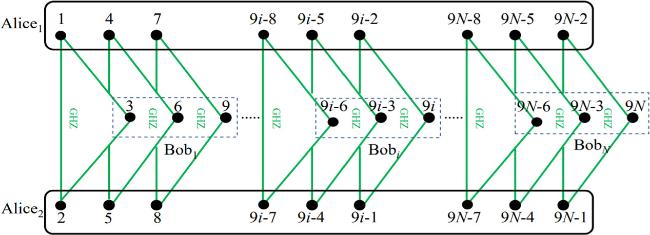
Figure 3. Distribution of shared qubits in the multicast scheme of three qubits. |
Step 1. Alice1 performs projective measurement {∣μi⟩, i = 0, ⋯ , 23N − 1} on her 3N qubits based on the amplitude coefficients, as follows:
$\begin{eqnarray}\left(\begin{array}{c}| {\mu }_{0}\rangle \\ | {\mu }_{1}\rangle \\ \vdots \\ | {\mu }_{{2}^{3N}-1}\rangle \end{array}\right)=\left(\underset{k=1}{\overset{N}{\displaystyle \bigotimes }}{\eta }_{k}\right)\left(\begin{array}{c}| 00\ldots 00\rangle \\ | 00\ldots 01\rangle \\ \vdots \\ | 11\ldots 11\rangle \end{array}\right),\end{eqnarray}$
where the three-qubit unitary operation ηk is $\begin{eqnarray}{\eta }_{k}=\left(\begin{array}{cccccccc}{a}_{k} & {b}_{k} & {c}_{k} & {d}_{k} & {e}_{k} & {f}_{k} & {g}_{k} & {h}_{k}\\ {b}_{k} & -{a}_{k} & {d}_{k} & -{c}_{k} & {f}_{k} & -{e}_{k} & {h}_{k} & -{g}_{k}\\ {c}_{k} & -{d}_{k} & -{a}_{k} & {b}_{k} & -{g}_{k} & {h}_{k} & {e}_{k} & -{f}_{k}\\ {d}_{k} & {c}_{k} & -{b}_{k} & -{a}_{k} & {h}_{k} & {g}_{k} & -{f}_{k} & -{e}_{k}\\ {e}_{k} & -{f}_{k} & {g}_{k} & -{h}_{k} & -{a}_{k} & {b}_{k} & -{c}_{k} & {d}_{k}\\ {f}_{k} & {e}_{k} & -{h}_{k} & -{g}_{k} & -{b}_{k} & -{a}_{k} & {d}_{k} & {c}_{k}\\ {g}_{k} & -{h}_{k} & -{e}_{k} & {f}_{k} & {c}_{k} & -{d}_{k} & -{a}_{k} & {b}_{k}\\ {h}_{k} & {g}_{k} & {f}_{k} & {e}_{k} & -{d}_{k} & -{c}_{k} & -{b}_{k} & -{a}_{k}\end{array}\right).\end{eqnarray}$
Assume that the measurement result of Alice1 is i1i2 ⋯ i3N, and the corresponding decimal expression is r.Step 2. Alice2 makes projective measurement based on the result r of Alice1 and phase information. The projective measurement is also denoted by $\{| {\nu }_{i}^{r}\rangle ,i=0,\cdots ,\,{2}^{3N}-1\}$, as follows:
$\begin{eqnarray}\begin{array}{l}{\left(\begin{array}{cccc}| {\nu }_{0}^{r}\rangle & | {\nu }_{1}^{r}\rangle & \cdots & | {\nu }_{{2}^{3N}-1}^{r}\rangle \end{array}\right)}^{{\rm{T}}}\\ =\underset{k=1}{\overset{N}{\bigotimes }}({X}^{({i}_{3k-1}\oplus {i}_{3k})\wedge {i}_{3k-1}}\otimes {X}^{{i}_{3k-2}\wedge {i}_{3k}}\otimes {X}^{{i}_{3k-2}\vee {i}_{3k-1}}){\zeta }_{k}({X}^{{i}_{3k-2}}\otimes {X}^{{i}_{3k-1}}\otimes {X}^{{i}_{3k}})\\ \cdot {\left(\begin{array}{cccc}| 00\ldots 00\rangle & | 00\ldots 01\rangle & \cdots & | 11\ldots 11\rangle \end{array}\right)}^{{\rm{T}}},\end{array}\end{eqnarray}$
where the superscript T means transposition of the matrix, and the three-qubit operation ζk has the following form: $\begin{eqnarray}{\zeta }_{k}=\displaystyle \frac{1}{2\sqrt{2}}\left(\begin{array}{cccccccc}{{\rm{e}}}^{-{\rm{i}}{\alpha }_{k}} & {{\rm{e}}}^{-{\rm{i}}{\beta }_{k}} & {{\rm{e}}}^{-{\rm{i}}{\gamma }_{k}} & {{\rm{e}}}^{-{\rm{i}}{\delta }_{k}} & {{\rm{e}}}^{-{\rm{i}}{\epsilon }_{k}} & {{\rm{e}}}^{-{\rm{i}}{\zeta }_{k}} & {{\rm{e}}}^{-{\rm{i}}{\eta }_{k}} & {{\rm{e}}}^{-{\rm{i}}{\theta }_{k}}\\ {{\rm{e}}}^{-{\rm{i}}{\alpha }_{k}} & -{{\rm{e}}}^{-{\rm{i}}{\beta }_{k}} & {{\rm{e}}}^{-{\rm{i}}{\gamma }_{k}} & -{{\rm{e}}}^{-{\rm{i}}{\delta }_{k}} & {{\rm{e}}}^{-{\rm{i}}{\epsilon }_{k}} & -{{\rm{e}}}^{-{\rm{i}}{\zeta }_{k}} & {{\rm{e}}}^{-{\rm{i}}{\eta }_{k}} & -{{\rm{e}}}^{-{\rm{i}}{\theta }_{k}}\\ {{\rm{e}}}^{-{\rm{i}}{\alpha }_{k}} & {{\rm{e}}}^{-{\rm{i}}{\beta }_{k}} & -{{\rm{e}}}^{-{\rm{i}}{\gamma }_{k}} & -{{\rm{e}}}^{-{\rm{i}}{\delta }_{k}} & {{\rm{e}}}^{-{\rm{i}}{\epsilon }_{k}} & {{\rm{e}}}^{-{\rm{i}}{\zeta }_{k}} & -{{\rm{e}}}^{-{\rm{i}}{\eta }_{k}} & -{{\rm{e}}}^{-{\rm{i}}{\theta }_{k}}\\ {{\rm{e}}}^{-{\rm{i}}{\alpha }_{k}} & -{{\rm{e}}}^{-{\rm{i}}{\beta }_{k}} & -{{\rm{e}}}^{-{\rm{i}}{\gamma }_{k}} & {{\rm{e}}}^{-{\rm{i}}{\delta }_{k}} & {{\rm{e}}}^{-{\rm{i}}{\epsilon }_{k}} & -{{\rm{e}}}^{-{\rm{i}}{\zeta }_{k}} & -{{\rm{e}}}^{-{\rm{i}}{\eta }_{k}} & {{\rm{e}}}^{-{\rm{i}}{\theta }_{k}}\\ {{\rm{e}}}^{-{\rm{i}}{\alpha }_{k}} & {{\rm{e}}}^{-{\rm{i}}{\beta }_{k}} & {{\rm{e}}}^{-{\rm{i}}{\gamma }_{k}} & {{\rm{e}}}^{-{\rm{i}}{\delta }_{k}} & -{{\rm{e}}}^{-{\rm{i}}{\epsilon }_{k}} & -{{\rm{e}}}^{-{\rm{i}}{\zeta }_{k}} & -{{\rm{e}}}^{-{\rm{i}}{\eta }_{k}} & -{{\rm{e}}}^{-{\rm{i}}{\theta }_{k}}\\ {{\rm{e}}}^{-{\rm{i}}{\alpha }_{k}} & -{{\rm{e}}}^{-{\rm{i}}{\beta }_{k}} & {{\rm{e}}}^{-{\rm{i}}{\gamma }_{k}} & -{{\rm{e}}}^{-{\rm{i}}{\delta }_{k}} & -{{\rm{e}}}^{-{\rm{i}}{\epsilon }_{k}} & {{\rm{e}}}^{-{\rm{i}}{\zeta }_{k}} & -{{\rm{e}}}^{-{\rm{i}}{\eta }_{k}} & {{\rm{e}}}^{-{\rm{i}}{\theta }_{k}}\\ {{\rm{e}}}^{-{\rm{i}}{\alpha }_{k}} & {{\rm{e}}}^{-{\rm{i}}{\beta }_{k}} & -{{\rm{e}}}^{-{\rm{i}}{\gamma }_{k}} & -{{\rm{e}}}^{-{\rm{i}}{\delta }_{k}} & -{{\rm{e}}}^{-{\rm{i}}{\epsilon }_{k}} & -{{\rm{e}}}^{-{\rm{i}}{\zeta }_{k}} & {{\rm{e}}}^{-{\rm{i}}{\eta }_{k}} & {{\rm{e}}}^{-{\rm{i}}{\theta }_{k}}\\ {{\rm{e}}}^{-{\rm{i}}{\alpha }_{k}} & -{{\rm{e}}}^{-{\rm{i}}{\beta }_{k}} & -{{\rm{e}}}^{-{\rm{i}}{\gamma }_{k}} & {{\rm{e}}}^{-{\rm{i}}{\delta }_{k}} & -{{\rm{e}}}^{-{\rm{i}}{\epsilon }_{k}} & {{\rm{e}}}^{-{\rm{i}}{\zeta }_{k}} & {{\rm{e}}}^{-{\rm{i}}{\eta }_{k}} & -{{\rm{e}}}^{-{\rm{i}}{\theta }_{k}}\end{array}\right).\end{eqnarray}$
The binary expression of Alice2's measurement result is denoted as j1j2 ⋯ j3N.Step 3. Based on the measurement results of Alice1 and Alice2, Bobk (where k = 1, 2, ⋯ , N) makes recovery operation on his three qubits according to the following formula:
$\begin{eqnarray}\begin{array}{l}{Z}_{9k-6}^{{j}_{3k-2}}{\left({ZX}\right)}_{9k-6}^{{i}_{3k-2}}\otimes {Z}_{9k-3}^{{j}_{3k-1}}{\left({ZX}\right)}_{9k-3}^{{i}_{3k-1}}\\ \otimes {Z}_{9k}^{{j}_{3k}}{\left({ZX}\right)}_{9k}^{{i}_{3k}}.\end{array}\end{eqnarray}$
Note. Because of the unitary property of quantum operation, it is difficult to find out a general formula for the recovery operation for the three-qubit case if we use methods similar to the two-qubit case. That is, the three-qubit case is not a simple generalization of the two-qubit case. We perform both row and column transformations on matrix ζk to overcome this difficulty.Similarly, we take an example to illustrate the three-qubit quantum multicast protocol. For example, when N = 3, the measurement result of Alice1 is 010 101 110, and its decimal representation is 174. That is, Alice1 measures her qubits in the basis:
$\begin{eqnarray}\begin{array}{l}| {\mu }_{174}\rangle \\ =\,({c}_{1}| 000\rangle -{d}_{1}| 001\rangle -{a}_{1}| 010\rangle +{b}_{1}| 011\rangle -{g}_{1}| 100\rangle \\ \,+\,{h}_{1}| 101\rangle +{e}_{1}| 110\rangle -{f}_{1}| 111\rangle )\\ \otimes \,({f}_{2}| 000\rangle +{e}_{2}| 001\rangle -{h}_{2}| 010\rangle -{g}_{2}| 011\rangle -{b}_{2}| 100\rangle \\ \,-\,{a}_{2}| 101\rangle +{d}_{2}| 110\rangle +{c}_{2}| 111\rangle )\\ \otimes \,({g}_{3}| 000\rangle -{h}_{3}| 001\rangle -{e}_{3}| 010\rangle +{f}_{3}| 011\rangle +{c}_{3}| 100\rangle \\ \,-\,{d}_{3}| 101\rangle -{a}_{3}| 110\rangle +{b}_{3}| 111\rangle ).\end{array}\end{eqnarray}$
Alice2 performs the following measurement according to the result of Alice1: $\begin{eqnarray}\begin{array}{l}{\left(\begin{array}{cccc}| {\nu }_{0}^{174}\rangle & | {\nu }_{1}^{174}\rangle & \cdots & | {\nu }_{{2}^{9}-1}^{174}\rangle \end{array}\right)}^{{\rm{T}}}\\ =\,\left((X\otimes I\otimes X){\zeta }_{1}(I\otimes X\otimes I)\right)\\ \,\otimes \left((I\otimes X\otimes X){\zeta }_{2}(X\otimes I\otimes X)\right)\\ \otimes \,\left((X\otimes I\otimes X){\zeta }_{3}(X\otimes X\otimes I)\right)\cdot {\left(\begin{array}{cccc}| 00\ldots 00\rangle & | 00\ldots 01\rangle & \cdots & | 11\ldots 11\rangle \end{array}\right)}^{{\rm{T}}}.\end{array}\end{eqnarray}$
Assuming that the measurement result of Alice2 is 101 010 100 (randomly selected), the collapsed state of the system after measurement is $\begin{eqnarray}\begin{array}{l}\left({c}_{1}{{\rm{e}}}^{{\rm{i}}{\gamma }_{1}}| 000\rangle -{d}_{1}{{\rm{e}}}^{{\rm{i}}{\delta }_{1}}| 001\rangle -{a}_{1}{{\rm{e}}}^{{\rm{i}}{\alpha }_{1}}| 010\rangle +{b}_{1}{{\rm{e}}}^{{\rm{i}}{\beta }_{1}}| 011\rangle -{g}_{1}{{\rm{e}}}^{{\rm{i}}{\eta }_{1}}| 100\rangle \right.\\ {\left.+\,{h}_{1}{{\rm{e}}}^{{\rm{i}}{\theta }_{1}}| 101\rangle +{e}_{1}{{\rm{e}}}^{{\rm{i}}{\epsilon }_{1}}| 110\rangle -{f}_{1}{{\rm{e}}}^{{\rm{i}}{\zeta }_{1}}| 111\rangle \right)}_{3,6,9}\otimes \left(-{f}_{2}{{\rm{e}}}^{{\rm{i}}{\zeta }_{2}}| 000\rangle +{e}_{2}{{\rm{e}}}^{{\rm{i}}{\epsilon }_{2}}| 001\rangle \right.\\ +\,{h}_{2}{{\rm{e}}}^{{\rm{i}}{\theta }_{2}}| 010\rangle -{g}_{2}{{\rm{e}}}^{{\rm{i}}{\eta }_{2}}| 011\rangle +{b}_{2}{{\rm{e}}}^{{\rm{i}}{\beta }_{2}}| 100\rangle -{a}_{2}{{\rm{e}}}^{{\rm{i}}{\alpha }_{2}}| 101\rangle -{d}_{2}{{\rm{e}}}^{{\rm{i}}{\delta }_{2}}| 110\rangle \\ {\left.+\,{c}_{2}{{\rm{e}}}^{{\rm{i}}{\gamma }_{2}}| 111\rangle \right)}_{12,15,18}\left({g}_{3}{{\rm{e}}}^{{\rm{i}}{\eta }_{3}}| 011\rangle +{h}_{3}{{\rm{e}}}^{{\rm{i}}{\theta }_{3}}| 010\rangle -{e}_{3}{{\rm{e}}}^{{\rm{i}}{\epsilon }_{3}}| 001\rangle -{f}_{3}{{\rm{e}}}^{{\rm{i}}{\zeta }_{3}}| 000\rangle \right.\\ {\left.+\,{c}_{3}{{\rm{e}}}^{{\rm{i}}{\gamma }_{3}}| 111\rangle +{d}_{3}{{\rm{e}}}^{{\rm{i}}{\delta }_{3}}| 110\rangle -{a}_{3}{{\rm{e}}}^{{\rm{i}}{\alpha }_{3}}| 101\rangle -{b}_{3}{{\rm{e}}}^{{\rm{i}}{\beta }_{3}}| 100\rangle \right)}_{21,24,27}.\end{array}\end{eqnarray}$
The recovery operations of Bob1, Bob2 and Bob3 are Z3 ⨂ Z6X6 ⨂ Z9, Z12X12 ⨂ I15 ⨂ Z18X18 and X21 ⨂ Z24X24 ⨂ I27, respectively. It is clear that all the receivers can obtain the desired state.3. Experimental simulation of quantum multicast in IBMQ
In this section, we present the quantum state tomography of the theoretical scheme of the quantum multicast in section 2 . The theoretical and experimental density matrices are compared to analyze the effectiveness of the quantum multicast schemes.
3.1. Quantum state tomography and fidelity
The core idea of quantum state tomography is to reconstruct the density matrix by preparing a large number of identical states and measuring them on a different basis [1, 61]. For a given N-qubit state ∣φ⟩, the theoretical density matrix is expressed as
$\begin{eqnarray}{\rho }^{{T}}=| \varphi \rangle \langle \varphi | .\end{eqnarray}$
The experimental density matrix of an N-qubit state is given by $\begin{eqnarray}{\rho }^{{E}}=\displaystyle \frac{1}{{2}^{N}}\displaystyle \sum _{{k}_{1},{k}_{2},\cdots ,{k}_{N}=0}^{3}{T}_{{k}_{1},{k}_{2},\cdots ,{k}_{N}}({\sigma }_{{k}_{1}}\otimes {\sigma }_{{k}_{2}}\otimes \cdots \otimes {\sigma }_{{k}_{N}}),\end{eqnarray}$
where ${\sigma }_{{k}_{i}},\,\mathrm{where}\,i=1,2,\cdots ,\,N$, means the Pauli matrix operating on the ith qubit. ${T}_{{k}_{1},{k}_{2},\cdots ,{k}_{N}}$ represents the result of a particular measurement as $\begin{eqnarray}{T}_{{k}_{1},{k}_{2},\cdots ,{k}_{N}}={S}_{{k}_{1}}\times {S}_{{k}_{2}}\,\times \cdots \times \,{S}_{{k}_{N}},\end{eqnarray}$
where ${S}_{{k}_{1}}\times {S}_{{k}_{2}}\times \cdots \times {S}_{{k}_{N}}$ are the Stokes parameters, and k1, k2, ⋯ ,kN take the values 0, 1, 2 and 3, which correspond to the quantum gates I, X, Y and Z, respectively. The Stokes parameters are S0 = P∣0I⟩ + P∣1I⟩, S1 = P∣0X⟩ − P∣1X⟩, S2 = P∣0Y⟩ − P∣1Y⟩ and S3 = P∣0Z⟩ − P∣1Z⟩. P∣0I⟩ is the probability of result ∣0⟩ when the qubit is measured in I basis, and P∣1I⟩ is the probability of result ∣1⟩ when the qubit is measured in I basis. The other pairs (P∣0X⟩, P∣1X⟩), (P∣0Y⟩, P∣1Y⟩) and (P∣0Z⟩, P∣1Z⟩) have similar meaning, but the qubits are measured in X, Y and Z bases, respectively [61].To analyze the gap between the theoretical and experimental results, we calculated the fidelity between the theoretical matrix ρT and experimental density matrix ρE, as follows:
$\begin{eqnarray}F({\rho }^{{T}},{\rho }^{{E}})=\mathrm{Tr}\sqrt{\sqrt{{\rho }^{{T}}}{\rho }^{{E}}\sqrt{{\rho }^{{T}}}},\end{eqnarray}$
where $\sqrt{A}$ is the square root of positive matrix A, and $\mathrm{Tr}$ is the trace of the matrix [1].3.2. Experimental results
In this subsection, we show the experimental results from the IBMQ platform [62–64]. For the single-, two- and three-qubit quantum multicast, we choose two specific states for each scheme. The two states have the same amplitude information but different phase information. The experimental density matrices with real and imaginary parts are shown.
3.2.1. Result for the quantum multicast of the single-qubit state
In this part, the multicast was between Alice1, Alice2 and Bob1, Bob2, corresponding to the scheme in section 2.1 when N = 2. The theoretical state was chosen as $| {\varphi }_{1}^{1}\rangle =(| 0\rangle +{\rm{i}}| 1\rangle )/\sqrt{2}$ and $| {\varphi }_{2}^{1}\rangle =(| 0\rangle +| 1\rangle )/\sqrt{2}$, with an imaginary part in state $| {\varphi }_{1}^{1}\rangle $. The density matrices of the experimental states were
$\begin{eqnarray}{\rho }_{1}^{{E}}=\left(\begin{array}{cc}0.4982 & 0.0039\\ 0.0039 & 0.5018\end{array}\right)+{\rm{i}}\left(\begin{array}{cc}0 & -0.5\\ 0.5 & 0\end{array}\right),\end{eqnarray}$
and $\begin{eqnarray}{\rho }_{2}^{{E}}=\left(\begin{array}{cc}0.4922 & 0.5\\ 0.5 & 0.5078\end{array}\right)+{\rm{i}}\left(\begin{array}{cc}0 & -0.0033\\ 0.0033 & 0\end{array}\right).\end{eqnarray}$
These are also shown in figure 4. The fidelities for states $| {\varphi }_{1}^{1}\rangle $ and $| {\varphi }_{2}^{1}\rangle $ both approached 1, as follows: $\begin{eqnarray}F(| {\varphi }_{1}^{1}\rangle ,{\rho }_{1}^{{E}})=| \langle {\varphi }_{1}^{1}| {\rho }_{1}^{{E}}| {\varphi }_{1}^{1}\rangle | \,\approx \,1.0000,\end{eqnarray}$
and $\begin{eqnarray}\quad F(| {\varphi }_{2}^{1}\rangle ,{\rho }_{2}^{{E}})=| \langle {\varphi }_{2}^{1}| {\rho }_{2}^{{E}}| {\varphi }_{2}^{1}\rangle | \,\approx \,1.0000.\end{eqnarray}$
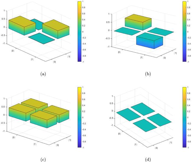
Figure 4. Real and imaginary parts of the experimental density matrices for the single-qubit multicast. (a) and (b) Real and imaginary parts of the experimental density matrix of $| {\varphi }_{1}^{1}\rangle $. (c) and (d) Real and imaginary parts of the experimental density matrix of $| {\varphi }_{2}^{1}\rangle $. |
3.2.2. Result for the quantum multicast of the two-qubit state
The experimental scheme of the quantum multicast for the two-qubit state was also applied to the two-receiver case. The theoretical states Bob1 and Bob2 wanted to obtain were
$\begin{eqnarray}| {\varphi }_{1}^{2}\rangle =\displaystyle \frac{1}{2}(| 00\rangle +{\rm{i}}| 01\rangle +{\rm{i}}| 10\rangle +| 11\rangle ),\end{eqnarray}$
and $\begin{eqnarray}| {\varphi }_{2}^{2}\rangle =\displaystyle \frac{1}{2}(| 00\rangle +| 01\rangle +| 10\rangle +| 11\rangle ),\end{eqnarray}$
respectively. The experimental density matrices were $\begin{eqnarray}\begin{array}{l}{\rho }_{1}^{{E}}=\left(\begin{array}{cccc}0.2424 & -0.0021 & -0.0011 & -0.0055\\ -0.0021 & 0.2485 & 0.0056 & -0.0011\\ -0.0011 & 0.0056 & 0.2513 & -0.0022\\ -0.0055 & -0.0011 & -0.0022 & 0.2577\end{array}\right)\\ \quad +{\rm{i}}\left(\begin{array}{cccc}0 & -0.0055 & -0.2469 & 0.0022\\ 0.0055 & 0 & 0.0021 & -0.2531\\ 0.2469 & -0.0021 & 0 & -0.0057\\ -0.0022 & 0.2531 & 0.0057 & 0\end{array}\right)\end{array}\end{eqnarray}$
and $\begin{eqnarray}\begin{array}{l}{\rho }_{2}^{{E}}=\left(\begin{array}{cccc}0.2498 & -9.9468{\rm{e}}-04 & 0.0021 & -4.0889{\rm{e}}-05\\ -9.9468{\rm{e}}-04 & 0.2595 & 2.4199{\rm{e}}-05 & 0.0022\\ 0.0021 & 2.4199{\rm{e}}-05 & 0.2407 & -9.5844{\rm{e}}-04\\ -4.0889{\rm{e}}-05 & 0.0022 & -9.5844{\rm{e}}-04 & 0.2500\end{array}\right)\\ \quad +\,{\rm{i}}\left(\begin{array}{cccc}0 & -0.0032 & -0.0025 & -1.7106{\rm{e}}-05\\ 0.0032 & 0 & 3.7134{\rm{e}}-05 & -0.0026\\ 0.0025 & -3.7134{\rm{e}}-05 & 0 & -0.0031\\ 1.7106{\rm{e}}-05 & 0.0026 & 0.0031 & 0\end{array}\right).\end{array}\end{eqnarray}$
The real and imaginary parts of the experimental density matrices are shown in figure 5. The fidelities between the theoretical and experimental density matrices were $\begin{eqnarray}F(| {\varphi }_{1}^{2}\rangle ,{\rho }_{1}^{{E}})=| \langle {\varphi }_{1}^{2}| {\rho }_{1}^{{E}}| {\varphi }_{1}^{2}\rangle | \,\approx \,0.7015,\end{eqnarray}$
and $\begin{eqnarray}\quad F(| {\varphi }_{2}^{2}\rangle ,{\rho }_{2}^{{E}})=| \langle {\varphi }_{2}^{2}| {\rho }_{2}^{{E}}| {\varphi }_{2}^{2}\rangle | \,\approx \,0.5012.\end{eqnarray}$
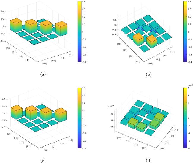
Figure 5. Real and imaginary parts of the experimental density matrices for the two-qubit multicast. (a) and (b) Real and imaginary parts of the experimental density matrix of $| {\varphi }_{1}^{2}\rangle $. (c) and (d) Real and imaginary parts of the experimental density matrix of $| {\varphi }_{2}^{2}\rangle $. |
3.2.3. Result for the quantum multicast of the three-qubit state
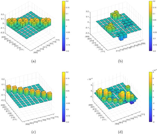
For the three-qubit case, we still chose to have two receivers, Bob1 and Bob2, at the same time. The theoretical states Bob1 and Bob2 wanted to get were
$\begin{eqnarray}\begin{array}{l}| {\varphi }_{1}^{3}\rangle =\displaystyle \frac{1}{2\sqrt{2}}(| 000\rangle +| 001\rangle +{\rm{i}}| 010\rangle \\ \quad +\,{\rm{i}}| 011\rangle +| 100\rangle \\ \quad +| 101\rangle +{\rm{i}}| 110\rangle +| 111\rangle ),\end{array}\end{eqnarray}$
and $\begin{eqnarray}\begin{array}{l}| {\varphi }_{2}^{3}\rangle =\displaystyle \frac{1}{2\sqrt{2}}(| 000\rangle +| 001\rangle +| 010\rangle +| 011\rangle +| 100\rangle \\ \,+\,| 101\rangle +| 110\rangle +| 111\rangle ),\end{array}\end{eqnarray}$
respectively. The experimental density matrices were $\begin{eqnarray}\begin{array}{l}{\rho }_{1}^{{E}}=\left(\begin{array}{cccccccc}0.1215 & 0.0932 & 0.0292 & 0.0205 & 0.0017 & 0.0013 & 0.0016 & 0.0012\\ 0.0932 & 0.1251 & 0.0243 & 0.0300 & 0.0013 & 0.0017 & 0.0012 & 0.0016\\ 0.0292 & 0.0243 & 0.1251 & 0.0960 & -0.0008 & -0.0006 & 0.0017 & 0.0014\\ 0.0205 & 0.0300 & 0.0960 & 0.1289 & -0.0006 & -0.0008 & 0.0013 & 0.0018\\ 0.0017 & 0.0013 & -0.0008 & -0.0006 & 0.1212 & 0.0930 & 0.0291 & 0.0204\\ 0.0013 & 0.0017 & -0.0006 & -0.0008 & 0.0930 & 0.1248 & 0.0242 & 0.0300\\ 0.0016 & 0.0012 & 0.0017 & 0.0013 & 0.0291 & 0.0242 & 0.1248 & 0.0958\\ 0.0012 & 0.0016 & 0.0014 & 0.0018 & 0.0204 & 0.0300 & 0.0958 & 0.1286\end{array}\right)\\ \quad \quad +\,{\rm{i}}\left(\begin{array}{cccccccc}0 & -0.0025 & -0.0923 & -0.0715 & 0.0015 & 0.0011 & -0.0009 & -0.0007\\ 0.0025 & 0 & -0.0703 & -0.0951 & 0.0012 & 0.0016 & -0.0007 & -0.0009\\ 0.0923 & 0.0703 & 0 & -0.0026 & 0.0017 & 0.0013 & 0.0016 & 0.0012\\ 0.0715 & 0.0951 & 0.0026 & 0 & 0.0013 & 0.0017 & 0.0013 & 0.0016\\ -0.0015 & -0.0012 & -0.0017 & -0.0013 & 0 & -0.0025 & -0.0921 & -0.0713\\ -0.0011 & -0.0016 & -0.0013 & -0.0017 & 0.0025 & 0 & -0.0701 & -0.0949\\ 0.0009 & 0.0007 & -0.0016 & -0.0013 & 0.0921 & 0.0701 & 0 & -0.0026\\ 0.0007 & 0.0009 & -0.0012 & -0.0016 & 0.0713 & 0.0949 & 0.0026 & 0\end{array}\right),\end{array}\end{eqnarray}$
and $\begin{eqnarray}\begin{array}{l}{\rho }_{2}^{{E}}=\left(\begin{array}{cccccccc}0.1229 & 0.0008 & 0.0033 & 1.7759{\rm{e}}-05 & -0.0004 & -3.5073{\rm{e}}-06 & -1.2396{\rm{e}}-05 & -9.7418{\rm{e}}-08\\ 0.0008 & 0.1255 & 2.235{\rm{e}}-05 & 0.0033 & -1.3640{\rm{e}}-06 & -0.0004 & -5.5468{\rm{e}}-08 & -1.2653{\rm{e}}-05\\ 0.0033 & 2.235{\rm{e}}-05 & 0.1215 & 0.0007 & -8.5024{\rm{e}}-06 & -8.8163{\rm{e}}-08 & -0.0004 & -3.4664{\rm{e}}-06\\ 1.7759{\rm{e}}-05 & 0.0033 & 0.0007 & 0.1240 & -1.6702{\rm{e}}-08 & -8.6786{\rm{e}}-06 & -1.3481{\rm{e}}-06 & -0.0004\\ -0.0004 & -1.3640{\rm{e}}-06 & -8.5024{\rm{e}}-06 & -1.6702{\rm{e}}-08 & 0.1260 & 0.0008 & 0.0033 & 1.8198{\rm{e}}-05\\ -3.5073{\rm{e}}-06 & -0.0004 & -8.8163{\rm{e}}-08 & -8.6786{\rm{e}}-06 & 0.0008 & 0.1286 & 2.2904{\rm{e}}-05 & 0.0034\\ -1.2396{\rm{e}}-05 & -5.5468{\rm{e}}-08 & -0.0004 & -1.3481{\rm{e}}-06 & 0.0033 & 2.2904{\rm{e}}-05 & 0.1245 & 0.0008\\ -9.7418{\rm{e}}-08 & -1.2653{\rm{e}}-05 & -3.4664{\rm{e}}-06 & -0.0004 & 1.8198{\rm{e}}-05 & 0.0034 & 0.0008 & 0.1271\end{array}\right)\\ +\,{\rm{i}}\left(\begin{array}{cccccccc}0 & -0.0004 & -0.0007 & -1.4844{\rm{e}}-05 & -0.0003 & -7.9439{\rm{e}}-07 & -6.5409{\rm{e}}-06 & -5.5871{\rm{e}}-10\\ 0.0004 & 0 & 6.0128{\rm{e}}-06 & -0.0007 & -3.3274{\rm{e}}-06 & -0.0003 & -8.0086{\rm{e}}-08 & -6.6764{\rm{e}}-06\\ 0.0007 & -6.0128{\rm{e}}-06 & 0 & -0.0004 & -1.1142{\rm{e}}-05 & -4.1447{\rm{e}}-08 & -0.0003 & -7.8513{\rm{e}}-07\\ 1.4844{\rm{e}}-05 & 0.0007 & 0.0004 & 0 & -9.5977{\rm{e}}-08 & -1.1373{\rm{e}}-05 & -3.2887{\rm{e}}-06 & -0.0003\\ 0.0003 & 3.3274{\rm{e}}-06 & 1.1142{\rm{e}}-05 & 9.5977{\rm{e}}-08 & 0 & -0.0004 & -0.0007 & -1.5211{\rm{e}}-05\\ 7.9439{\rm{e}}-07 & 0.0003 & 4.1447{\rm{e}}-08 & 1.1373{\rm{e}}-05 & 0.0004 & 0 & 6.1614{\rm{e}}-06 & -0.0007\\ 6.5409{\rm{e}}-06 & 8.0086{\rm{e}}-08 & 0.0003 & 3.2887{\rm{e}}-06 & 0.0007 & -6.1614{\rm{e}}-06 & 0 & -0.0004\\ 5.8571{\rm{e}}-10 & 6.6764{\rm{e}}-06 & 7.8513{\rm{e}}-07 & 0.0003 & 1.5211{\rm{e}}-05 & 0.0007 & 0.0004 & 0\end{array}\right).\end{array}\end{eqnarray}$
The real and imaginary parts of the experimental density matrices are shown in figure 6. The fidelities between the theoretical and experimental density matrices were $\begin{eqnarray}F(| {\varphi }_{1}^{3}\rangle ,{\rho }_{1}^{{E}})=| \langle {\varphi }_{1}^{3}| {\rho }_{1}^{{E}}| {\varphi }_{1}^{3}\rangle | \,\approx \,0.3048,\end{eqnarray}$
and $\begin{eqnarray}\quad F(| {\varphi }_{2}^{3}\rangle ,{\rho }_{2}^{{E}})=| \langle {\varphi }_{2}^{3}| {\rho }_{2}^{{E}}| {\varphi }_{2}^{3}\rangle | \,\approx \,0.1829.\end{eqnarray}$
Figure 6. Real and imaginary parts of the experimental density matrices for the three-qubit multicast. (a) and (b) Real and imaginary parts of the experimental density matrix of $| {\varphi }_{1}^{3}\rangle $. (c) and (d) Real and imaginary parts of the experimental density matrix of $| {\varphi }_{2}^{3}\rangle $. |
4. Efficiency and fidelity analysis
In this subsection, we analyze the efficiency and fidelity of our scheme, compare the efficiency of our results with existing results and discuss the effects of different types of noise.
4.1. Efficiency analysis
The efficiency of quantum communication scheme is defined as [65]
$\begin{eqnarray}\eta =\displaystyle \frac{{q}_{p}}{{q}_{c}+{x}_{t}},\end{eqnarray}$
where qp represents the number of qubits to be transmitted, qc indicates the number of qubits used in the quantum scheme and xt denotes the number of classical bits needed. As far as we know, very little research has been conducted on three-qubit quantum multicast. Therefore, we compared our results with others in two ways: first, by comparing them with JRSP of three-qubit states, and second, by comparing them with the quantum multicast of single qubits.In table 1, we compared our scheme with the existing three-qubit JRSP scheme from the second to sixth row. The efficiency of our scheme is better than 1/7 in [33] and 3/17 in [66]. Moreover, we need to mention that the transmitted state in [67] was a special three-qubit state with five complex coefficients. The target state in [68] was a three-qubit equatorial state with equal amplitudes. However, our scheme holds true for any three-qubit state with eight complex coefficients. We compared our one-qubit quantum multicast scheme with that in [57] from the seventh to eighth row. Our scheme was applied to the N-qubit GHZ state with any coefficient (whether real or complex). The scheme in [57] was applied only to the real case.
Table 1. Communication efficiency comparison with other existing JRSP or quantum multicast schemes. |
| Scheme | qp | qc | xt | η |
|---|---|---|---|---|
| JRSP in [33] | Arbitrary three-qubit state | 12 | 9 | 1/7 |
| | ||||
| JRSP in [66] | Arbitrary three-qubit state | 10 | 7 | 3/17 |
| | ||||
| JRSP in [67] | Three-qubit state with five coefficients | 9 | 6 | 1/5 |
| | ||||
| JRSP in [68] | Three-qubit equatorial state | 9 | 6 | 1/5 |
| | ||||
| Our scheme as JRSP (N = 1) | Arbitrary three-qubit state | 9 | 6 | 1/5 |
| | ||||
| Quantum multicast in [57] | n number of N-qubit GHZ state | (N − 1)n + 2n + 1 | 2n | $\tfrac{{Nn}}{{Nn}+3n+1}$ |
| | ||||
| Our quantum multicast | n number of N-qubit GHZ state | 3n + (N − 1)n | 2n | $\tfrac{{nN}}{{Nn}+5n}$ |
4.2. Effects of noise
In this subsection, we discuss the effects of noise on the multicast protocol. We considered two types of noise. The first was white noise. The second type of noise was generated during the particle distribution process.
4.2.1. Effect of the white noise
Assume that the elementary cell of the shared channel is not the maximally entangled GHZ state; it is the three-qubit generalized Werner state [69]:
$\begin{eqnarray}{\rho }_{w}=p\left|\mathrm{GHZ}\right\rangle \left\langle \mathrm{GHZ}\right|+(1-p)\displaystyle \frac{1}{8}I,\quad p\in (0,1),\end{eqnarray}$
which is a mixture of the GHZ state and the white noise. Consider a single-qubit multicast scheme as an example. For simplicity of calculation, let us consider the case of three receivers as an example. The general N case result can be obtained through induction.The shared channel (or the initial state of the whole system) is a composite of three generalized Werner states:
$\begin{eqnarray}\begin{array}{l}{\rho }_{s}={\left({\rho }_{w}\right)}_{123}\otimes {\left({\rho }_{w}\right)}_{456}\otimes {\left({\rho }_{w}\right)}_{789}\\ ={p}^{3}{\left(| \mathrm{GHZ}\rangle \langle \mathrm{GHZ}| \right)}^{\otimes 3}\\ \,+\,{\left(1-p\right)}^{3}{\left(\displaystyle \frac{1}{8}I\right)}^{\otimes 3}+\displaystyle \frac{{p}^{2}(1-p)}{8}\left[{\left(| \mathrm{GHZ}\rangle \langle \mathrm{GHZ}| \right)}^{\otimes 2}\otimes I\right.\\ \left.\quad +| \mathrm{GHZ}\rangle \langle \mathrm{GHZ}| \otimes I\otimes | \mathrm{GHZ}\rangle \langle \mathrm{GHZ}| +I\otimes {\left(| \mathrm{GHZ}\rangle \langle \mathrm{GHZ}| \right)}^{\otimes 2}\right]\\ \,+\,\displaystyle \frac{{\left(1-p\right)}^{3}}{64}{I}^{\otimes 3}\\ \quad +\,\displaystyle \frac{p{\left(1-p\right)}^{2}}{64}\left[| \mathrm{GHZ}\rangle \langle \mathrm{GHZ}| \otimes {I}^{\otimes 2}+I\otimes | \mathrm{GHZ}\rangle \langle \mathrm{GHZ}| \otimes I+{I}^{\otimes 2}\otimes | \mathrm{GHZ}\rangle \langle \mathrm{GHZ}| \right].\end{array}\end{eqnarray}$
Here, the qubits are labeled from 1 to 9, from left to right. Alice1 possesses qubits 1, 4 and 7. Alice2 has qubits 2, 5 and 8. Bob1, Bob2 and Bob3 hold qubits 3, 6 and 9, respectively. Alice1 and Alice2 want to help Bobi obtain the state $| {\varphi }_{i}\rangle ={a}_{i}| 0\rangle +{b}_{i}{{\rm{e}}}^{{\rm{i}}{\theta }_{i}}| 1\rangle $, where i = 1, 2, 3.Assume that Alice1's measurement on qubits 1, 4 and 7 in step 1 is
$\begin{eqnarray}| {\mu }_{0}{\rangle }_{147}=({a}_{1}| 0\rangle +{b}_{1}| 1\rangle )({a}_{2}| 0\rangle +{b}_{2}| 1\rangle )({a}_{3}| 0\rangle +{b}_{3}| 1\rangle ).\end{eqnarray}$
The collapsed state of the whole system is $\begin{eqnarray}\begin{array}{l}{\rho }_{0}=\displaystyle \frac{{\mathrm{Tr}}_{147}\left[| {\mu }_{0}\rangle \langle {\mu }_{0}| {\rho }_{s}{\left(| {\mu }_{0}\rangle \langle {\mu }_{0}| \right)}^{\dagger }\right]}{\mathrm{Tr}\left[| {\mu }_{0}\rangle \langle {\mu }_{0}| {\rho }_{s}{\left(| {\mu }_{0}\rangle \langle {\mu }_{0}| \right)}^{\dagger }\right]}\\ =\,{p}^{3}{\otimes }_{i=1}^{3}| {{\rm{\Psi }}}_{i}\rangle \langle {{\rm{\Psi }}}_{i}| +{p}^{2}(1-p)\left[| {{\rm{\Psi }}}_{1}\rangle \langle {{\rm{\Psi }}}_{1}| \otimes | {{\rm{\Psi }}}_{2}\rangle \langle {{\rm{\Psi }}}_{2}| \otimes \displaystyle \frac{I}{4}+| {{\rm{\Psi }}}_{1}\rangle \langle {{\rm{\Psi }}}_{1}| \otimes \displaystyle \frac{I}{4}\otimes | {{\rm{\Psi }}}_{3}\rangle \langle {{\rm{\Psi }}}_{3}| \right.\\ \left.\quad +\,\displaystyle \frac{I}{4}\otimes | {{\rm{\Psi }}}_{2}\rangle \langle {{\rm{\Psi }}}_{2}| \otimes \otimes | {{\rm{\Psi }}}_{3}\rangle \langle {{\rm{\Psi }}}_{3}| \right]+p{\left(1-p\right)}^{2}\left[| {{\rm{\Psi }}}_{1}\rangle \langle {{\rm{\Psi }}}_{1}| \otimes {\left(\displaystyle \frac{I}{4}\right)}^{\otimes 2}+\displaystyle \frac{I}{4}\otimes | {{\rm{\Psi }}}_{2}\rangle \langle {{\rm{\Psi }}}_{2}| \otimes \displaystyle \frac{I}{4}\right.\\ \left.\quad +\,{\left(\displaystyle \frac{I}{4}\right)}^{\otimes 2}| {{\rm{\Psi }}}_{3}\rangle \langle {{\rm{\Psi }}}_{3}| \right]+{\left(1-p\right)}^{3}{\left(\displaystyle \frac{I}{4}\right)}^{\otimes 3},\end{array}\end{eqnarray}$
where ${\mathrm{Tr}}_{147}$ means the partial trace on qubits 1, 4 and 7, and ∣$\Psi$i⟩ = ai∣00⟩ + bi∣11⟩, where i = 1, 2, 3.Alice1 sends her measurement result to Alice2 by three classical bits. According to Alice1's result, Alice2 chooses to do measurement $\{| {\nu }_{j}^{0}\rangle ,j=0,1,2,3\}$ on her qubits 2, 5 and 8. Assume that Alice2's measurement result is $| {\nu }_{0}^{0}\rangle $, and the collapsed state of Bob1, Bob2 and Bob3 is
$\begin{eqnarray}\begin{array}{l}{\rho }_{0}^{0}=\displaystyle \frac{{\mathrm{Tr}}_{258}\left[| {\nu }_{0}^{0}\rangle \langle {\nu }_{0}^{0}| {\rho }_{0}{\left(| {\nu }_{0}^{0}\rangle \langle {\nu }_{0}^{0}| \right)}^{\dagger }\right]}{\mathrm{Tr}\left[| {\nu }_{0}^{0}\rangle \langle {\nu }_{0}^{0}| {\rho }_{0}{\left(| {\nu }_{0}^{0}\rangle \langle {\nu }_{0}^{0}| \right)}^{\dagger }\right]}\\ =\,{p}^{3}{\otimes }_{i=1}^{3}| {\varphi }_{i}\rangle \langle {\varphi }_{i}| +{p}^{2}(1-p)\left[| {\varphi }_{1}\rangle \langle {\varphi }_{1}| \otimes | {\varphi }_{2}\rangle \langle {\varphi }_{2}| \otimes \displaystyle \frac{I}{2}+| {\varphi }_{1}\rangle \langle {\varphi }_{1}| \otimes \displaystyle \frac{I}{2}\otimes | {\varphi }_{3}\rangle \langle {\varphi }_{3}| \right.\\ \left.\quad +\,\displaystyle \frac{I}{2}\otimes | {\varphi }_{2}\rangle \langle {\varphi }_{2}| \otimes \otimes | {\varphi }_{3}\rangle \langle {\varphi }_{3}| \right]+p{\left(1-p\right)}^{2}\left[| {\varphi }_{1}\rangle \langle {\varphi }_{1}| \otimes {\left(\displaystyle \frac{I}{2}\right)}^{\otimes 2}+\displaystyle \frac{I}{2}\otimes | {\varphi }_{2}\rangle \langle {\varphi }_{2}| \otimes \displaystyle \frac{I}{2}\right.\\ \left.\quad +{\left(\displaystyle \frac{I}{2}\right)}^{\otimes 2}| {\varphi }_{3}\rangle \langle {\varphi }_{3}| \right]+{\left(1-p\right)}^{3}{\left(\displaystyle \frac{I}{2}\right)}^{\otimes 3}.\end{array}\end{eqnarray}$
Note that for the other measurement results of Alice1 and Alice2, the output state is the same as ${\rho }_{0}^{0}$ after the recovery operations of Bob1, Bob2 and Bob3. For each Bobk (where k = 1, 2, 3), the system state is $\begin{eqnarray}{\rho }_{0k}^{0}={p}^{3}| {\varphi }_{k}\rangle \langle {\varphi }_{k}| +{p}^{2}(1-p)\left[2| {\varphi }_{k}\rangle \langle {\varphi }_{k}| +\displaystyle \frac{I}{2}\right]+p{\left(1-p\right)}^{2}\left[| {\varphi }_{k}\rangle \langle {\varphi }_{k}| +I\right]+{\left(1-p\right)}^{3}\displaystyle \frac{I}{2}.\end{eqnarray}$
As a result, the fidelity between the target and the output state of the whole system for the three-receiver case is
$\begin{eqnarray}{F}_{3}=\left|\langle {\varphi }_{1}| \langle {\varphi }_{2}| \langle {\varphi }_{3}| {\rho }_{0}^{0}| {\varphi }_{1}\rangle | {\varphi }_{2}\rangle | {\varphi }_{3}\rangle \right|={\left(\displaystyle \frac{1+p}{2}\right)}^{3}.\end{eqnarray}$
Using a similar method, it is easy to conclude that the fidelity FN = (1 + p)N/2N for the N-receiver case. Note that for the shared channel with white noise, the fidelity is independent of the input classical information. This is affected by the noise rate and the number of receivers. The fidelity decreases with the number of receivers and is 1/2N when the channel is in the maximally mixed state. However, if we consider each receiver independently, the fidelity always remains the same and does not change with the number of receivers. The fidelity of receiver Bobk is $\begin{eqnarray}{F}^{k}=\left|\langle {\varphi }_{k}| {\rho }_{0k}^{0}| {\varphi }_{k}\rangle \right|=\displaystyle \frac{1+p}{2}.\end{eqnarray}$
4.2.2. Effect of noise from the particle distribution process
Here, we discuss the effect of the noise generated during the particle distribution process. Assume that there is an entanglement state generator that generates GHZ states and distributes them to Alice1, Alice2 and Bobk, where k = 1, 2, ⋯ , N. In the particle distribution process, the ith particle is subjected to noise ${{ \mathcal E }}_{i}$, which is expressed in terms of Kraus operators as ${{ \mathcal E }}_{i}(\rho )={\sum }_{{j}_{i}}{E}_{{j}_{i}}\rho {E}_{{j}_{i}}^{\dagger }$.
For a comprehensive understanding, we considered a single-qubit quantum multicast scheme as an example. For simplicity of calculation, we assumed that all of the particles were subjected to the same kind of noise, for example, bit-flip noise. We selected the simplest case, where N = 2. The shared channel after the particle distribution was
$\begin{eqnarray}\begin{array}{l}{ \mathcal E }(| \mathrm{GHZ}\rangle \langle \mathrm{GHZ}{| }^{\otimes 2})={{ \mathcal E }}_{1}\otimes \cdots \otimes {{ \mathcal E }}_{6}(| \mathrm{GHZ}\rangle \langle \mathrm{GHZ}{| }^{\otimes 2})\\ =\displaystyle \sum _{{j}_{1},\cdots ,{j}_{6}}({E}_{{j}_{1}}\otimes \cdots \otimes {E}_{{j}_{6}})(| \mathrm{GHZ}\rangle \langle \mathrm{GHZ}{| }^{\otimes 2}){\left({E}_{{j}_{1}}\otimes \cdots \otimes {E}_{{j}_{6}}\right)}^{\dagger }.\end{array}\end{eqnarray}$
Here, ${{ \mathcal E }}_{i}(\rho )={{ \mathcal E }}_{{BF}}(\rho )={E}_{0}\rho {E}_{0}^{\dagger }+{E}_{1}\rho {E}_{1}^{\dagger }=(1-\lambda )I\rho I+\lambda X\rho X$, with λ the probability of flipping qubit ∣0⟩ to ∣1⟩ and vice versa [1]. By direct calculation, we obtained the shared channel, as follows: $\begin{eqnarray}\begin{array}{l}{\rho }_{s}={ \mathcal E }(| \mathrm{GHZ}\rangle \langle \mathrm{GHZ}{| }^{\otimes 2})\\ =\,\{[{\lambda }^{3}+{\left(1-\lambda \right)}^{3}]| \mathrm{GHZ}\rangle \langle \mathrm{GHZ}| +\lambda (1-\lambda )\\ \,(| {{\rm{G}}}_{1}\rangle \langle {{\rm{G}}}_{1}| +| {{\rm{G}}}_{2}\rangle \langle {{\rm{G}}}_{2}| +| {{\rm{G}}}_{3}\rangle \langle {{\rm{G}}}_{3}| )\}{}^{\otimes 2},\end{array}\end{eqnarray}$
where $\begin{eqnarray*}\begin{array}{l}| {{\rm{G}}}_{1}\rangle =\displaystyle \frac{1}{\sqrt{2}}(| 001\rangle +| 110\rangle ),\quad | {{\rm{G}}}_{2}\rangle =\displaystyle \frac{1}{\sqrt{2}}(| 010\rangle +| 101\rangle ),\quad | {{\rm{G}}}_{3}\rangle =\displaystyle \frac{1}{\sqrt{2}}(| 011\rangle +| 100\rangle ).\end{array}\end{eqnarray*}$
Assuming that the measurement result of Alice1 is ∣μ0⟩14 = (a1∣0⟩ + b1∣1⟩)(a2∣0⟩ + b2∣1⟩), the remaining system state after the measurement is
$\begin{eqnarray}\begin{array}{l}{\rho }_{0}=\displaystyle \frac{{\mathrm{Tr}}_{14}\left[| {\mu }_{0}\rangle \langle {\mu }_{0}| {\rho }_{s}{\left(| {\mu }_{0}\rangle \langle {\mu }_{0}| \right)}^{\dagger }\right]}{\mathrm{Tr}\left[| {\mu }_{0}\rangle \langle {\mu }_{0}| {\rho }_{s}{\left(| {\mu }_{0}\rangle \langle {\mu }_{0}| \right)}^{\dagger }\right]}\\ =\,{\otimes }_{k=1}^{2}\left\{[{\lambda }^{3}+{\left(1-\lambda \right)}^{3}]| {\phi }_{0}^{k}\rangle \langle {\phi }_{0}^{k}| +\lambda (1-\lambda )\left[| {\phi }_{1}^{k}\rangle \langle {\phi }_{1}^{k}| \right.\right.\\ \,\left.\left.\,+| {\phi }_{2}^{k}\rangle \langle {\phi }_{2}^{k}| +| {\phi }_{3}^{k}\rangle \langle {\phi }_{3}^{k}| \right]\right\},\end{array}\end{eqnarray}$
with $\begin{eqnarray*}| {\phi }_{0}^{k}\rangle ={a}_{k}| 00\rangle +{b}_{k}| 11\rangle ,\quad | {\phi }_{1}^{k}\rangle ={a}_{k}| 01\rangle +{b}_{k}| 10\rangle ,\end{eqnarray*}$
$\begin{eqnarray*}| {\phi }_{2}^{k}\rangle ={a}_{k}| 10\rangle +{b}_{k}| 01\rangle ,\quad | {\phi }_{3}^{k}\rangle ={a}_{k}| 11\rangle +{b}_{k}| 00\rangle .\end{eqnarray*}$
After receiving the measurement result of Alice1, Alice2 chooses measurement $\{| {\nu }_{j}^{0}\rangle ,j=0,1,2,3\}$. Assuming that the measurement result of Alice2 is $| {\nu }_{0}^{0}\rangle $, then the remaining system state of Bob1 and Bob2 is
$\begin{eqnarray}\begin{array}{l}{\rho }_{0}^{0}=\displaystyle \frac{{\mathrm{Tr}}_{25}\left[| {\nu }_{0}^{0}\rangle \langle {\nu }_{0}^{0}| {\rho }_{0}{\left(| {\nu }_{0}^{0}\rangle \langle {\nu }_{0}^{0}| \right)}^{\dagger }\right]}{\mathrm{Tr}\left[| {\nu }_{0}^{0}\rangle \langle {\nu }_{0}^{0}| {\rho }_{0}{\left(| {\nu }_{0}^{0}\rangle \langle {\nu }_{0}^{0}| \right)}^{\dagger }\right]}\\ \,=\,{\otimes }_{k=1}^{2}\left\{[{\lambda }^{3}+{\left(1-\lambda \right)}^{3}]| {\varphi }_{0}^{k}\rangle \langle {\varphi }_{0}^{k}| +\lambda (1-\lambda )\left[| {\varphi }_{1}^{k}\rangle \langle {\varphi }_{1}^{k}| \right.\right.\\ \,\left.\left.\,+| {\varphi }_{2}^{k}\rangle \langle {\varphi }_{2}^{k}| +| {\varphi }_{3}^{k}\rangle \langle {\varphi }_{3}^{k}| \right]\right\},\end{array}\end{eqnarray}$
where $\begin{eqnarray*}| {\varphi }_{0}^{k}\rangle ={a}_{k}| 0\rangle +{b}_{k}{{\rm{e}}}^{{\rm{i}}{\theta }_{k}}| 1\rangle ,\quad | {\varphi }_{1}^{k}\rangle ={a}_{k}| 1\rangle +{b}_{k}{{\rm{e}}}^{{\rm{i}}{\theta }_{k}}| 0\rangle ,\end{eqnarray*}$
$\begin{eqnarray*}| {\varphi }_{2}^{k}\rangle ={a}_{k}{{\rm{e}}}^{{\rm{i}}{\theta }_{k}}| 0\rangle +{b}_{k}| 1\rangle ,\quad | {\varphi }_{3}^{k}\rangle ={a}_{k}{{\rm{e}}}^{{\rm{i}}{\theta }_{k}}| 1\rangle +{b}_{k}| 0\rangle .\end{eqnarray*}$
The state of Bobk is $\begin{eqnarray}\begin{array}{l}{\rho }_{0k}^{0}=[{\lambda }^{3}+{\left(1-\lambda \right)}^{3}]| {\varphi }_{0}^{k}\rangle \langle {\varphi }_{0}^{k}| \\ +\,\lambda (1-\lambda )\left[| {\varphi }_{1}^{k}\rangle \langle {\varphi }_{1}^{k}| +| {\varphi }_{2}^{k}\rangle \langle {\varphi }_{2}^{k}| +| {\varphi }_{3}^{k}\rangle \langle {\varphi }_{3}^{k}| \right].\end{array}\end{eqnarray}$
As a result, the state-dependent fidelity of the two-receiver quantum multicast is
$\begin{eqnarray}\begin{array}{l}{F}_{2}({\varphi }_{1},{\varphi }_{2})=\left|\langle {\varphi }_{1}| \langle {\varphi }_{2}| {\rho }_{0}^{0}| {\varphi }_{1}\rangle | {\varphi }_{2}\rangle \right|\\ =\,\left[1+\lambda (1-\lambda )(4{a}_{1}^{2}{b}_{1}^{2}\cos 2{\theta }_{1}+4{a}_{1}^{2}{b}_{1}^{2}-2)\right]\\ \cdot \left[1+\lambda (1-\lambda )(4{a}_{2}^{2}{b}_{2}^{2}\cos 2{\theta }_{2}+4{a}_{2}^{2}{b}_{2}^{2}-2)\right].\end{array}\end{eqnarray}$
The state-dependent fidelity from the angle of Bobk is $\begin{eqnarray}\begin{array}{l}{F}^{k}=\left|\langle {\varphi }_{k}| {\rho }_{0k}^{0}| {\varphi }_{k}\rangle \right|\\ =\,\left[1+\lambda (1-\lambda )(4{a}_{k}^{2}{b}_{k}^{2}\cos 2{\theta }_{k}+4{a}_{k}^{2}{b}_{k}^{2}-2)\right]\end{array}\end{eqnarray}$
If we let ${a}_{k}=\cos \tfrac{{\omega }_{k}}{2}$, ${b}_{k}=\sin \tfrac{{\omega }_{k}}{2}$ and ωk ∈ [0, 2π], where k = 1, 2, we can get the average fidelity of each Bobk: $\begin{eqnarray}F=\,\displaystyle \frac{1}{4\pi }{\int }_{0}^{\pi }\sin {\theta }_{k}{\rm{d}}{\theta }_{k}{\int }_{0}^{2\pi }{F}^{k}{\rm{d}}{\omega }_{k}=\,1-\displaystyle \frac{5}{3}\lambda (1-\lambda ).\end{eqnarray}$
Note that, if there are N receivers, the state-dependent and average fidelities are the same as those of the two-receiver case for each Bobk. The average fidelity attains its minimum of 7/12 when λ = 1/2, which corresponds to the most uncertain case of the bit-flip channel.5. Conclusions and discussions
In this study, we considered the problem of transmitting quantum information from two senders to multiple receivers, i.e. quantum multicast. The theoretical schemes were completed based on JRSP using GHZ states as shared channels. The contributions of this study are as follows:
(a) Theoretical protocols for the quantum multicast of arbitrary single, two and three qubits have been presented. Using the idea of JRSP, we split the information of the target state into the amplitude and phase parts. Three-qubit GHZ states were chosen as the shared channels. The number of GHZ states depends on the number of target qubits and receivers. The quantum multicast was completed in three steps. First, one sender made projective measurements based on the amplitude information and sent the measurement results to the other sender. Second, the remaining sender constructed projective measurements according to the results of the first sender. Finally, according to the results of the senders, the receivers performed Pauli operations on their qubits to recover the target. All protocols are deterministic in the sense that they can be completed with 100% probability in an ideal environment.
(b) Experimental simulations of the theoretical protocols for specific states were performed on the IBMQ platform. In the simulation section, we selected the case of two receivers for all the single-, two- and three-qubit protocols. One target state contained complex phase information, whereas the other did not. The amplitude information was the same for both target states. The fidelity between the theoretical and experimental states was close to 1 for the single-qubit multicast and greater than one-half for the two-qubit multicast.
(c) The efficiency and effects of noise have been discussed for the quantum multicast scheme. When we consider only the one-receiver case, our protocol is actually a JRSP protocol. The communication efficiency of our protocol was greater than or equal to that of previous studies for a three-qubit state. When the white noise was introduced into our scheme, the fidelity of each receiver was the same and had relation only with the noise rate. When the noise was induced by the particle distribution process, we presented a calculation model for the single-qubit multicast with two receivers. We found that for the bit-flip noise, the average fidelity was only affected by the noise rate. The fidelity attained its minimum when the noise was in the most uncertain situation.
(d) The most important highlight of this study is that we propose a quantum multicast scheme for any three qubits, regardless of whether the parameters of the three-qubit state are real or complex, which, to the best of our knowledge, has not been investigated. The fidelity of the three-qubit state with complex coefficients is approximately 0.3084.
We compared our results with those of previous studies on quantum multicast. Zhao et al [57] exhibited the multicast of N-qubit GHZ-type states using 2N-qubit entangled state as the shared channel. They first completed the multicast of N real coefficient single qubits, and then prepared the N-qubit GHZ-type states by CNOT gates based on the obtained single qubits. Peng et al [59] considered the multicast of two four-qubit states with four complex coefficients, using two six-qubit nonmaximally entangled states as shared channels and five auxiliary qubits. In [60], the authors presented a multicast of two complex two-qubit states with the help of a maximally entangled nine-qubit state and four auxiliary qubits. They also gave the multicast of two arbitrary single qubits using a six-qubit maximally entangled channel [70]. In [71], using nonmaximally entangled channels, the authors presented two multicast schemes for two real coefficient states. The first scheme was with two four-qubit cluster-type states as the target states, each with four coefficients. This was completed according to a certain probability. The second scheme was with one single-qubit and one two-qubit states as the target states and can be completed deterministically in theory. In [72], the multicast of N real-coefficient single qubits was discussed using the composite of N Bell states. For clarity, these comparisons are listed in table 2. In table 2, we listed seven aspects of the multicast schemes. OR in table 2 is the abbreviation for our result. The first row of column ‘1' is the number of target states, column ‘2' is the qubit number of target states, column ‘3' is whether the coefficients of the target states are real or complex (where R means real and C means complex), column ‘4' is the qubit number of the shared channel, column ‘5' is whether the shared channel is maximally entangled or not (where M means maximally entagled and NM nonmaximally), column ‘6' is the number of auxiliary qubits and column ‘7' is whether the scheme is probabilistic or deterministic (where P means probabilistic and D deterministic).
Table 2. Comparison between our results and those of previous studies. |
In conclusion, we focused mainly on the quantum multicast of single, two and three qubits. It would also be interesting to study the relationships between different entangled resources. Some equivalent conditions can be defined to classify multicast protocols that may convert to each other in the existing physical experimental environment, which may provide a valuable reference for physicists. The experimental realization of three-qubit GHZ states in different physical environments has been reported by many research groups, such as using superconducting phase qubits [73, 74], on NMR quantum information processor [75], in optical systems [76] and by photon scattering in one-dimensional waveguides [77]. Therefore, our protocol may have potential physically realizable value.