


1. Introduction
Regular black holes (BHs) were originally introduced as a means to circumvent the central singularity inherent in ordinary BHs. Regular BHs may be categorized into two types based on their asymptotic behavior approaching the center: those with a de Sitter (dS) core and those with a Minkowskian core. Notable examples of regular BHs with a dS core are the Bardeen BH [1], the Hayward BH [2] and the Frolov BH [3]. A regular BH with a Minkowskian core is usually characterized by exponential potentials, as described in references [4–13]. Comprehensive reviews on regular BHs can be found in references [14–16]. This research aims to analyze the characteristics of the quasinormal modes (QNMs) of Frolov BHs.
Perturbing a BH and observing its response is widely recognized as a powerful method for extracting the crucial characteristics of the BH. This perturbation can be implemented either by introducing a probe matter field into its spacetime by hand or by physically perturbing its metric. Perturbing the metric leads to the emission of gravitational waves (GWs). Prior to reaching equilibrium, the system undergoes a phase of BH merging, referred to as the ringdown phase. During this stage, the BH releases GWs with characteristic discrete frequencies, i.e. quasinormal frequencies (QNFs). These frequencies encode information about the decaying scales and damped oscillations of the BH [17]. Studying the properties of QNFs offers an opportunity to detect deviations from general relativity (GR) or even quantum gravity effects through observations of GWs. However, the majority of regular BHs are typically constructed by incorporating quantum gravity effects at the phenomenological level, making it challenging to establish consistently effective gravitational perturbation equations. Fortunately, even when only a probe matter field is considered over these regular BHs, their QNM spectra are also influenced by the background spacetime. Therefore, these QNM spectra also provide crucial information about the internal structure of the BH and can be used to model the form of the GW during the ringdown phase at a phenomenological level [18–22].
In [23], the authors investigated the properties of QNMs for a probe massless scalar field over a Frolov BH in the eikonal limit, i.e. a large angular quantum number. The effective potential for a Frolov BH is found to be higher than that of an uncharged Hayward BH. The imaginary parts of the QNFs for a Frolov BH grow with the charge and exhibit a maximum, followed by a more pronounced decrease for small values of the parameter associated with the effective cosmological constant at small distances. As the charge grows so do the real parts of the QNFs. In this work, we will conduct a systematic investigation of the QNMs of Frolov BHs, with a primary focus on the case of low angular quantum numbers, in contrast to the eikonal limit studied in [23].
Our paper is organized as follows. In section 2 , we offer a concise overview of Frolov BHs along with their fundamental properties, and we also introduce the dynamics of a scalar field over a Frolov BH. In section 3 , we provide a concise introduction to the pseudospectral method. The characteristics of the QNMs and ringdown waveforms of the scalar field over a Frolov BH are discussed in sections 4 and 5 , respectively. Conclusions and further discussions are presented in section 6 .
2. Probe scalar field over a Frolov black hole
A Frolov BH is an extension of a Hayward BH to the charged case, originally proposed in [3]. The geometry of a Frolov regular BH is described by [3]3 ). As α0 increases from the Schwarzschild BH case, the Hayward BH evolves into a BH with double horizons. On further increasing α0 to the upper bound defined by the inequality (3 ), the Hayward BH transforms into a BH with a single horizon. When q ≠ 0, with an increasing α0, the Frolov geometry, initially featuring double horizons, transitions to a spacetime with a single horizon (the middle plot in figure 1). Further increments in α0 lead to the development of a horizonless spacetime, often describing exotic compact objects (the middle plot in figure 1). However, when q is increased to q = 1, the Frolov geometry describes a horizonless spacetime for all α0 > 0 (the right plot in figure 1). Figure 2 displays the phase diagram of α0 versus q, illustrating the horizon structure of Frolov spacetime. In this paper, we will exclusively focus on studying the case of BH spacetime with horizons.
$\begin{eqnarray}{\rm{d}}{s}^{2}=-f(r){\rm{d}}{t}^{2}+\displaystyle \frac{1}{f(r)}{\rm{d}}{r}^{2}+{r}^{2}{\rm{d}}{\theta }^{2}+{r}^{2}{\sin }^{2}\theta {\rm{d}}{\phi }^{2},\end{eqnarray}$
$\begin{eqnarray}f(r)=1-\displaystyle \frac{(2{Mr}-{q}^{2}){r}^{2}}{{r}^{4}+(2{Mr}+{q}^{2}){\alpha }_{0}^{2}},\end{eqnarray}$
where M denotes the BH mass. This core of a Frolov BH is characterized by an effective cosmological constant ${\rm{\Lambda }}=3/{\alpha }_{0}^{2}$, where α0 represents the Hubble length. The Hubble length characterizes a universal hair and is bounded by the following inequality [2]: $\begin{eqnarray}{\alpha }_{0}\leqslant \sqrt{16/27}M.\end{eqnarray}$
Satisfying this constraint leads to significant quantum gravity effects. Subsequently, we will set M = 1 for simplicity, without loss of generality. The charge parameter q characterizes a specific hair and satisfies 0 ≤ q ≤ 1. At q = 0, a Frolov BH reduces to a Hayward BH, and at α0 = 0, it simplifies to a Reissner–Nordström (RN) BH. It is obvious that when both q = 0 and α0 = 0, a Frolov BH reduces to a Schwarzschild BH. Figure 1 shows the metric function f(r) of a Frolov BH for various q and α0. We begin by considering the case q = 0, corresponding to a Hayward BH (the left plot in figure 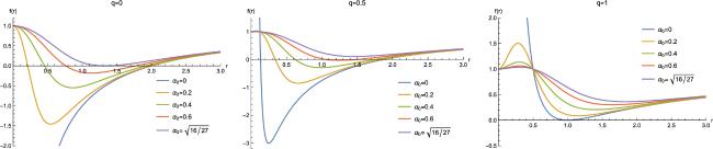
Figure 1. The metric function f(r) of a Frolov BH for various q and α0. |
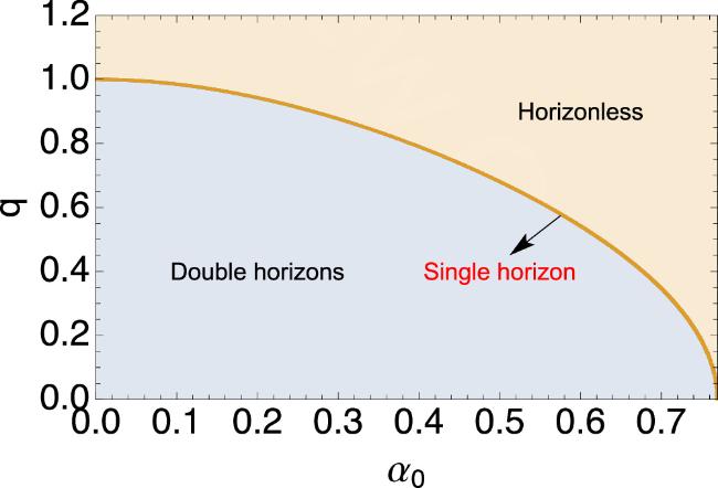
Figure 2. The phase diagram of α0 versus q, illustrating the horizon structure of Frolov spacetime. |
The Hawking temperature of a regular BH can be worked out as3 ) is satisfied. Figure 3 illustrates the relationship between the Hawking temperature and the charge parameter q for various values of α0 to aid visualization.
$\begin{eqnarray}\begin{array}{rcl}T & = & \displaystyle \frac{f^{\prime} ({r}_{h})}{4\pi }\\ & = & \displaystyle \frac{{r}_{h}\left(-{q}^{2}\left(2{\alpha }_{0}^{2}{r}_{h}+{r}_{h}^{4}\right)-4{\alpha }_{0}^{2}{r}_{h}^{2}+{r}_{h}^{5}+{\alpha }_{0}^{2}{q}^{4}\right)}{2\pi \left(2{\alpha }_{0}^{2}{r}_{h}+{r}_{h}^{4}+{\alpha }_{0}^{2}{q}^{2}\right){}^{2}}.\end{array}\end{eqnarray}$
Here, rh represents the event horizon of the BH. From the equation above, it is evident that when q = 0 and T = 0, the upper limit of equation (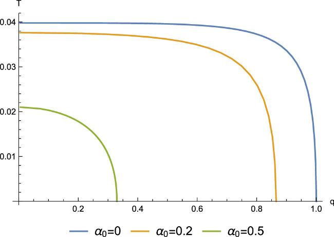
Figure 3. The Hawking temperature as a function of q with different α0. |
The dynamics of the probe scalar field can be described by the following Klein–Gordon (KG) equation:5 ) may be reformulated in the following manner:
$\begin{eqnarray}\displaystyle \frac{1}{\sqrt{-g}}{\partial }_{\nu }({g}^{\mu \nu }\sqrt{-g}{\partial }_{\mu }{\rm{\Phi }})=0.\end{eqnarray}$
Given the spherical symmetry of the geometry under investigation, we can employ the following spherical harmonics to separate the variables: $\begin{eqnarray}{\rm{\Phi }}(t,r,\theta ,\phi )=\displaystyle \sum _{l,m}{{\rm{Y}}}_{l,m}(\theta ,\phi )\displaystyle \frac{{{\rm{\Psi }}}_{l,m}(t,r)}{r},\end{eqnarray}$
In the above equation, Yl,m(θ, φ) is the spherical harmonics. Here, l and m stand for the angular and azimuthal quantum numbers, respectively. For a given l and m, we have simplified the notation by denoting $\Psi$l,m(t, r) as $\Psi$. Then the KG equation ( $\begin{eqnarray}-\displaystyle \frac{{\partial }^{2}{\rm{\Psi }}}{\partial {t}^{2}}+\displaystyle \frac{{\partial }^{2}{\rm{\Psi }}}{\partial {r}_{* }^{2}}-{V}_{\mathrm{eff}}{\rm{\Psi }}=0,\end{eqnarray}$
where r* is the tortoise coordinate associated with r, as dr*/dr = 1/f(r). The effective potential is given by: $\begin{eqnarray}{V}_{\mathrm{eff}}\,=\,f(r)\displaystyle \frac{l(l+1)}{{r}^{2}}+\displaystyle \frac{f(r)f^{\prime} (r)}{r},\end{eqnarray}$
with l = 0, 1, ….Figure 4 depicts the effective potential V(r*) for different BH parameters, namely α0 and q, with l = 0. For a fixed charge q, it is observed that as α0 increases, the peak value of the effective potential decreases, whereas the position of the peak remains almost unchanged (the left and middle plots in figure 4). The right-most plot in figure 4 shows the case of changing q with fixed α0 = 0.2. With an increase in q, both the peak value of the effective potential and its position consistently shift to the left. Moreover, it is noteworthy that, regardless of whether we vary α0 or q, there are discernible changes in the near-horizon behavior. These characteristics of the effective potential undoubtedly influence the behavior of the QNMs.
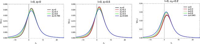
Figure 4. The effective potential V(r*) for various BH parameters α0 and charge parameters q with l = 0. |
3. Pseudospectral method
We will work in the Eddington–Finkelstein coordinate system and our study will be carried out in the frequency domain. To this end, we employ the following transformations:7 ) is then transformed into9 ), the metric function f(u) becomes
$\begin{eqnarray}r\to 1/u\ \ \mathrm{and}\ \ {\rm{\Psi }}={{\rm{e}}}^{-{\rm{i}}\omega {r}_{* }(u)}\psi .\end{eqnarray}$
Then we need to impose the ingoing and outgoing boundary condition at the horizon and infinity, respectively, $\begin{eqnarray}\psi \sim {{\rm{e}}}^{{\rm{i}}\omega {r}_{\ast }},\,\,\,\,\,{r}_{\ast }\to \infty .\end{eqnarray}$
Collecting the equations above, the wave equation ( $\begin{eqnarray}\begin{array}{l}(-l(l+1){u}^{2}-2{iu}(1-2(1+u)f(u)\\ +\,u(1+2u)f^{\prime} (u))\omega +4(1+2u)(1-f(u)\\ -\,2{uf}(u)){\omega }^{2})\psi (u)+({u}^{4}f^{\prime} (u)\\ +\,2{{\rm{i}}{u}}^{2}(1-(2+4u)f(u))\omega )\psi ^{\prime} (u)\\ +\,{u}^{4}f(u)\psi ^{\prime\prime} (u)=0,\end{array}\end{eqnarray}$
where the prime represents the derivative with respect to u. After the transformation ( $\begin{eqnarray}f(u)=1+\displaystyle \frac{u(-2+{q}^{2}u)}{1+2{u}^{3}{\alpha }_{0}^{2}+{q}^{2}{u}^{4}{\alpha }_{0}^{2}}.\end{eqnarray}$
Using the pseudospectral method to solve the eigenvalue problem in ω, the pivotal step involves discretizing the wave equation (11 ) (for more details, please refer to [24]). To achieve this, we employ the Chebyshev grids and Lagrange cardinal functions, defined as follows:
$\begin{eqnarray}\begin{array}{l}{u}_{i}=\cos \left(\displaystyle \frac{i}{N}\pi \right),\\ {C}_{j}(u)=\displaystyle \prod _{i=0,i\ne j}^{N}\displaystyle \frac{u-{u}_{i}}{{u}_{j}-{u}_{i}},i=0,...,N.\end{array}\end{eqnarray}$
Then, the function ψ(u) can be approximated as $\begin{eqnarray}\psi (u)\approx \displaystyle \sum _{j=0}^{N}f({u}_{j}){C}_{j}(u),\end{eqnarray}$
where the cardinal functions are linear combinations of Chebyshev polynomials Tn(u) of the first kind: $\begin{eqnarray}\begin{array}{l}{C}_{j}(u)=\displaystyle \frac{2}{{{Np}}_{j}}\displaystyle \sum _{m=0}^{N}\displaystyle \frac{1}{{p}_{m}}{T}_{m}({u}_{j}){T}_{m}(u),\\ {p}_{0}={p}_{N}=2,{p}_{j}=1.\end{array}\end{eqnarray}$
Afterwards, we can obtain the generalized eigenvalue equation in the form $\begin{eqnarray}\begin{array}{l}({M}_{0}+\omega {M}_{1})\psi =0,\end{array}\end{eqnarray}$
where Mi (i = 0, 1) represents the linear combination of the derivative matrices ${D}_{{ij}}^{(n)}={C}_{i}^{n}({u}_{j})$, where n represents the nth derivative matrix. By solving the eigenvalue function, we can determine the QNFs.4. Quasinormal modes
In this section, we will explore the characteristics of the QNMs on a Frolov BH. We illustrate the behavior of the fundamental modes in relation to the BH parameter α0 for various charge parameters q with l = 0 in figure 5 and l = 1 in figure 6. Additionally, for illustrative purposes, we present selected values of the fundamental modes corresponding to various BH parameters α0 and charge parameters q with l = 0 in table 1 and l = 1 in table 2. It is observed that the imaginary parts consistently reside in the lower half-plane. This suggests that a Frolov BH remains stable when subjected to scalar perturbations.

Figure 5. QNFs as a function of the BH parameter α0 for different charge parameters q with l = 0 and n = 0. |
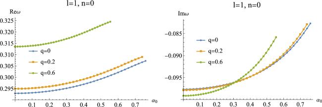
Figure 6. QNFs as a function of the BH parameter α0 for different charge parameters q with l = 1 and n = 0. |
Table 1. The fundamental modes for different BH parameters α0 and charge parameters q with l = 0. |
| q | $\omega \,\left({\alpha }_{0}=0\right)$ | $\omega \,\left({\alpha }_{0}=1/10\right)$ | $\omega \,\left({\alpha }_{0}=1/2\right)$ |
|---|---|---|---|
| 0 | 0.110 46–0.10490i | 0.110 61–0.10471i | 0.114 03–0.09889i |
| 2/10 | 0.111 24–0.10506i | 0.111 40–0.10486i | 0.114 87–0.09858i |
| 6/10 | 0.118 46–0.10593i | 0.118 67–0.10557i | 0.119 74–0.09271i |
Table 2. The fundamental modes for different BH parameters α0 and charge parameters q with l = 1. |
| q | $\omega \,\left({\alpha }_{0}=0\right)$ | $\omega \,\left({\alpha }_{0}=1/10\right)$ | $\omega \,\left({\alpha }_{0}=1/2\right)$ |
|---|---|---|---|
| 0 | 0.292 94–0.09766i | 0.293 18–0.09750i | 0.299 26–0.09287i |
| 2/10 | 0.294 94–0.09786i | 0.295 20–0.09769i | 0.301 55–0.09273i |
| 6/10 | 0.313 53–0.09915i | 0.313 90–0.09886i | 0.322 86–0.08913i |
Now we will delve deeper into studying some particular characteristics of the QNFs for the fundamental modes with respect to both the BH parameter α0 and the charge parameter q. When l = 0, there is a clear non-monotonic pattern in the real parts of the QNFs with respect to the BH parameter α0 for a given value of q (see the left plot in figure 5). The phenomenon of non-monotonic behavior has been documented in loop quantum gravity (LQG)-corrected BHs, as reported in [21, 22]. To be more precise, with an increase in the parameter α0, signifying that the system is farther from a Schwarzschild BH or a RN BH, the real parts of the QNFs initially go up, which means that the system is oscillating more strongly, and go down, which means that the oscillation is weakening. As the charge parameter q increases, the turning point of this non-monotonic behavior goes down. It is important to note that the real parts are smaller than that of a Schwarzschild BH or a RN BH as the parameter α0 increases. At the same time, as α0 increases so do the values of the imaginary parts of the QNFs, which points to a lower damping rate (see the right plot in figure 5). This result suggests that when quantum gravity effects are present we have a slower decay mode.
Furthermore, if we fix the BH parameter α0, we observe that in the region of small α0 the real parts of QNFs increase as the charge parameter q rises, indicating that the charge enhances the oscillation of the system. As the parameter α0 increases, we observe that the curves with q = 0.2 and q = 0.6 intersect (see the left plot in figure 5), suggesting an opposite trend in the change with q. The opposite change trend with q between small α0 and large α0 is more pronounced in the imaginary parts (see the right plot in figure 5). We also observe that when α0 is relatively large, the curves intersect again.
Next, we examine in detail the scenario when l = 1, as shown in figure 6. The non-monotonic behavior ceases to exist at l = 1. Specifically, both the real and imaginary parts consistently and continuously increase as the parameter α0 decreases. This means that the system oscillates more strongly and decays more slowly. We also analyzed the QNFs for the values of l > 1 and arrived at a similar result as in the case when l = 1. An analogous discovery has been documented with the fundamental modes of a LQG-corrected BH [22]. This means that the angular number has a bigger effect on the fundamental modes than quantum gravity effects. Further research should be done in the future into the universality of the non-monotonic behavior for l = 0 and the reasons behind this phenomenon.
5. Ringdown waveform
In this section we will investigate the time-domain profiles of the scalar field over a Frolov BH. To do this we need to solve numerically the time-dependent wave equation (7 ) using the following initial Gaussian wave packet:17 ) cannot influence the ringdown waveform. After the initial outburst stage, the ringdown waveform is fully determined by the QNMs, also called the quasinormal ringing stage.
$\begin{eqnarray}\begin{array}{rcl}{\rm{\Psi }}({r}_{* },t=0) & = & \exp \left[-\displaystyle \frac{{\left({r}_{* }-a\right)}^{2}}{2{b}^{2}}\right],\\ {\rm{\Psi }}({r}_{* },t\lt 0) & = & 0.\end{array}\end{eqnarray}$
Without loss of generality, we fix the tortoise coordinate at r* = 5. Notes that the different initial conditions (In figure 7 we display the semilogarithmic plots of the time-domain evolution of the scalar field for l = 0 and l = 1, showcasing various combinations of parameters q and α0. Notably, there is no increase in perturbation over time. Furthermore, we conduct a fitting analysis on the late-time tail decay, revealing a power-law behavior represented as $\Psi$ ∼ t−2l+3. These findings provide additional confirmation that a Frolov BH is dynamically stable when subjected to perturbations from a massless scalar field. This observation aligns with the findings from QNMs. Additionally, as a validation check we employ the Prony method to fit the fundamental mode; the results are presented in tables 3 and 4. These findings align with those obtained through the pseudospectral method, as presented in tables 1 and 2.

Figure 7. Semilogarithmic plots of the time-domain profiles of the scalar field for l = 0 and l = 1 with different parameters q and α0. |
Table 3. The fundamental modes obtained by the Prony method for different BH parameters α0 and charge parameters q with l = 0. |
| q | $\omega \,\left({\alpha }_{0}=0\right)$ | $\omega \,\left({\alpha }_{0}=1/10\right)$ | $\omega \,\left({\alpha }_{0}=1/2\right)$ |
|---|---|---|---|
| 0 | 0.110 89–0.10049i | 0.114 01–0.096998i | 0.115 34–0.092569i |
| 2/10 | 0.114 62–0.09729i | 0.114 69–0.097132i | 0.115 98–0.092354i |
| 6/10 | 0.111 60–0.10301i | 0.117 81–0.098063i | 0.118 52–0.086906i |
Table 4. The fundamental modes obtained by the Prony method for different BH parameters α0 and charge parameters q with l = 1. |
| q | $\omega \,\left({\alpha }_{0}=0\right)$ | $\omega \,\left({\alpha }_{0}=1/10\right)$ | $\omega \,\left({\alpha }_{0}=1/2\right)$ |
|---|---|---|---|
| 0 | 0.292 87–0.097679i | 0.293 01–0.097522i | 0.299 17–0.092926i |
| 2/10 | 0.294 78–0.097902i | 0.295 04–0.097735i | 0.301 46–0.092794i |
| 6/10 | 0.313 50–0.099311i | 0.313 87–0.099015i | 0.322 88–0.089244i |
6. Conclusions and discussions
In this paper we have investigated the properties of QNMs of the scalar field over a Frolov BH and have also provided a brief discussion on its time-domain evolution. A Frolov BH exhibits stability against scalar perturbations, as evidenced by the consistent presence of the imaginary parts of the QNMs in the lower half-plane and the gradual decay of perturbations over time.
When the angular quantum number l = 0, the real parts of QNFs display distinct non-monotonic behaviors. Specifically, with an increase in the BH parameter α0, the system undergoes stronger oscillations initially, followed by a weakening. The turning point of this non-monotonic behavior shifts downward as the charge parameter q increases. Furthermore, as the parameter α0 increases, the real parts become smaller compared to those of a Schwarzschild BH or RN BH. This suggests that, at this moment, the system undergoes weaker oscillations than a Schwarzschild BH or RN BH. The BH parameter α0 contributes to reducing the damping rate, as indicated by the increase in the values of the imaginary parts of the QNFs as α0 rises. This outcome suggests that the presence of quantum gravity effects leads to slower decay modes. We also briefly explore the impact of the charge parameter q. Our study indicates that the charge enhances the oscillations of the system. In addition, upon examining scenarios with higher angular quantum numbers (l ≥ 1), we observe the disappearance of the non-monotonic behavior observed in the case of l = 0. This disappearance may be attributed to the influence of the angular quantum number outweighing that of the quantum gravity effect. Further research is warranted to explore the universality of the non-monotonic behavior for l = 0.