


1. Introduction
The discovery of the late-time accelerated expansion of the Universe has become one of the most important theoretical challenges in modern cosmology. One of the first pieces of observational evidence of this late-time acceleration was obtained through the measurement of type Ia supernovae [1–3]. Subsequently, more observations such as the Sloan Digital Sky Survey (SDSS) and Wilkinson Microwave Anisotropy Probe (WMAP) [4], baryonic acoustic oscillations (BAO) [5] and cosmic microwave background (CMB) anisotropies [6–10] have confirmed that the Universe is spatially flat and two-thirds of the energy content is dominated by an exotic component with large negative pressure, referred to as dark energy. The simplest candidate for dark energy is the cosmological constant with its equation of state w = pΛ/ρΛ = −1. This model is known as the Lambda cold dark matter (ΛCDM) model which has three major components: a cosmological constant associated with dark energy, cold dark matter and ordinary matter. This model emerged in the late 1990s as a concordance model. Despite its observational success, the ΛCDM model suffers from at least two problems: the cosmological constant problem (CCP) and the cosmic coincidence problem [11, 12]. Many alternative theories have been proposed beyond the ΛCDM model to solve these conundrums. Generally, these alternative theories have been divided into two main classes: the first, and possibly the major class, is the dark energy model in which a new cosmic fluid or matter field is introduced within the framework of general relativity [13]. The other class is modified theories of gravity in which the standard general relativity Lagrangian is modified based on some concrete physical mechanism [14].
We are concerned here with the first kind of dark energy proposal, where the dark energy component might be explained by a background fluid with an exotic equation of state, the so-called the Chaplygin gas (CG) model [15]. The Chaplygin gas [16] had an origin that was not cosmological. It was used to explain the lifting force on an airplane wing. As the equation of state has negative pressure, it has recently attracted new interest in cosmology. It is used as a perfect fluid to describe the accelerating expansion of the Universe with equation of state pCh = −A/ρCh, where A is a positive constant, and pCh and ρCh are the energy density and pressure, respectively. The striking feature of the CG model is its ability to unify two of the Universe's unknown dark sections: dark matter (DM) and dark energy (DE) [17, 18]. Since the CG model was ruled out by observations, this model was extended to the so-called generalized Chaplygin gas (GCG) with equation of state [19] ${p}_{{Ch}}=-A/{\rho }_{{Ch}}^{\alpha }$, where 0 ≤ α ≤ 1. This GCG model is also regarded as a unification of DE and DM [20–23]. Gou and Zhang [24] have proposed a variable Chaplygin gas (VCG) model, which explains the evolution from dust to quintessence or phantom. In such a model, the equation of state is characterized by pCh = −A(a)/ρCh, where A is the function of the scale factor a. Yang et al [25], and later on, Lu [26] generalised the VCG model with equation of state ${p}_{{Ch}}=-A(a)/{\rho }_{{Ch}}^{\alpha }$, known the as variable generalized Chaplygin gas (VGCG) model, which also explains the evolution from dust to quintessence or phantom. Some more works on VCG and VGCG models can be found in [27–32]
Nevertheless, even in the context of general relativity, there are other theories to explain the current accelerated expansion of the Universe. As stated above, the presence of negative pressure is the main factor required to accelerate the expansion of the Universe. This may also occur, for instance, when the physical system departs from a thermodynamic equilibrium state [33]. In this connection, Zeldovich [34] first stated that the process of cosmological particle creation at the expense of the gravitational field can be phenomenologically described by a negative pressure. In cosmology, gravitationally induced particle production has a long history. Using the non-equilibrium thermodynamics of open systems, Prigogine et al [35, 36] proposed the first self-consistent macroscopic formulation of the matter creation process into the Einstein field equations. Later on, Calvâo et al [37] clarified the process through covariant formulation. It has been stated that matter creation can be explained in the realm of relativistic non-equilibrium thermodynamics. According to several studies [38–47], matter creation cosmology may explain the accelerating expansion of the Universe. The late-time evolution of the Universe has been explained by many authors [48–57]. Since many significant observations have been examined in recent years and the current accelerated expansion of the Universe is satisfactorily explained, matter creation cosmology is an extremely intriguing topic. The crucial aspect of this model is to take into account the option for the particle production rate, which is still unknown. However, it is assumed to be a function of the Hubble parameter H.
In our previous work [58], we mainly concentrated on the GCG inspired by matter creation cosmology and derived the best-fit values of model free parameters. In this paper, to make a more complete discussion on the contribution of matter creation in CG models, we are interested in discussing the consequences of a VGCG model incorporating the background of matter creation cosmology within the framework of a homogeneous and isotropic flat Friedmann–Lemaître–Robertson–Walker space-time. We also consider a special model of CG, namely, variable Chaplygin gas (VCG). We focus on the analytical solutions and observational analysis of the proposed models to explore the contribution of matter creation. To make our discussion more complete, we use a Bayesian analysis to constrain the parameter space of these models using BAO, cosmic chronometers data, Pantheon type Ia supernova including the gamma-ray bursts, quasars and local measurement of H0 from R21. It is worth noting that the VGCG and VCG models with matter creation can alleviate H0 tension. We also discuss the stability, Bayesian evidence analysis and selection criteria to distinguish our models from the existing dark energy models such as the ΛCDM model.
The paper is organized as follows: in section 2 , for the sake of clarity, we give a brief introduction to matter creation in cosmology. Section 3 is devoted to the background dynamics of the VGCG model with matter creation. The analytical solutions of VGCG and VCG models are presented in sections 4 and 5 , respectively. Recent observational data and posterior analysis are explored in section 6 . Section 7 is devoted to the results and discussion on the consistency of VGCG and VCG models with the observations. Further, sections 7.1 –7.4 present the evolutions of cosmological parameters, stability, information selection criteria and Bayesian evidence analysis, respectively, and finally, in section 8 , we present a summary of the results.
2. Basic formalism of matter creation
The thermodynamics of matter creation were first applied to cosmology in the late 1980s by Prigogine and collaborators [35, 36]. They included matter creation explicitly in the matter stress–energy tensor in the Einstein field equations. Later on, Calvâo et al [37] discussed and generalized this phenomenological approach through a covariant formulation allowing specific entropy variation. Nowadays, it is applied in many gravitational theories. In this paper we follow the approach of Prigogine et al [35, 36], which presumes that matter creation occurs at the expense of gravitational energy. The basic formalism of matter creation in the theory of general relativity is as follows.
Let us consider an open thermodynamical system where the number of particles is not conserved. The particle flux vector is assumed to have the form Nμ = nuμ, where N is the number of particles, n is the particle number density, given by n = N/V and uμ is the usual particle four-velocity. For open systems, the non-conservation of the particle number satisfies the balance equation2 ) can be rewritten as3 ) can be interpreted as a non-thermal pressure, known as creation pressure, defined as1 ) in equation (4 ), we get the following form of creation pressure [37]:6 ) in equation (5 ), the creation pressure gives
$\begin{eqnarray}{{\rm{\nabla }}}_{\mu }{N}^{\mu }\equiv {n}_{,\mu }{u}^{\mu }+3{Hn}=n{\rm{\Gamma }},\end{eqnarray}$
where Γ stands for the rate of change of the particle number in a physical volume V = V0a3 (where V0 is the co-moving volume) and ${u}_{;\mu }^{\mu }=3H$ denotes the fluid expansion for a Friedmann–Lemaître–Robertson–Walker (FLRW) Universe and by notation $\dot{n}={n}_{,\mu }{u}^{\mu }$. The overdot denotes derivative with respect to cosmic time. Clearly, Γ > 0 indicates the creation of particles while Γ < 0 stands for particle annihilation and Γ = 0 means there is no creation of matter, i.e., the particle number is conserved. The entropy flux vector is given by sμ = nσuμ [37], where σ is the specific (per particle) entropy. It is to be noted that the entropy must satisfy the second law of thermodynamics ${s}_{;\mu }^{\mu }\geqslant 0$. The incorporation of variable N into the cosmological scenario modifies the first law of thermodynamics as [36, 37] $\begin{eqnarray}{\rm{d}}(\rho V)+{p}{\rm{d}}{V}-(h/n){\rm{d}}({nV})=0,\end{eqnarray}$
where h = (ρ + p) is the enthalpy (per unit volume), and ρ and p are the energy density and thermodynamic pressure, respectively. It is assumed that the Universe evolution continues to be adiabatic, in the sense that the entropy per particle remains unchanged $(\dot{\sigma }=0)$. Equation ( $\begin{eqnarray}{\rm{d}}(\rho V)+(p+{p}_{c}){\rm{d}}{V}=0,\end{eqnarray}$
where the extra contribution pc in equation ( $\begin{eqnarray}{p}_{c}=-\displaystyle \frac{h}{n}\displaystyle \frac{{\rm{d}}({nV})}{{\rm{d}}{V}}.\end{eqnarray}$
Using equation ( $\begin{eqnarray}{p}_{c}=-\displaystyle \frac{(\rho +p)}{3H}{\rm{\Gamma }}.\end{eqnarray}$
Hence, the creation pressure pc can be identified with the particle production rate Γ. The simplest possible case, and probably the most physical choice would be one for which the characteristic time scale for matter creation is the Hubble time itself. Phenomenologically, this is equivalent to [59, 60] $\begin{eqnarray}{\rm{\Gamma }}=3\beta H,\end{eqnarray}$
where β is a positive constant. Using equation ( $\begin{eqnarray}{p}_{c}=-\beta (\rho +p).\end{eqnarray}$
Hereafter, we refer to ρ as ρCh and p as pCh for energy density and pressure of a CG perfect fluid.3. Basic field equations
Let us consider the following geometry of the Universe which is very well described by the homogeneous and isotropic flat FLRW space-time9 ) and equation (8 ), for line element, and equation (10 ), energy–momentum tensor, yield
$\begin{eqnarray}{{\rm{d}}{s}}^{2}=-{{\rm{d}}{t}}^{2}+{a}^{2}(t)\left({{\rm{d}}{r}}^{2}+{r}^{2}{\rm{d}}{\theta }^{2}+{r}^{2}{{\rm{\sin }}}^{2}\theta {\rm{d}}{\phi }^{2}\right),\end{eqnarray}$
where a(t) is the scale factor of the Universe. Throughout we use units such that the speed of light c = 1. For a co-moving observer, ${u}^{\mu }={\delta }_{\nu }^{\mu }$, in which uμuμ = −1. The Einstein field equations are written as $\begin{eqnarray}{R}_{\mu \nu }-\displaystyle \frac{1}{2}{g}_{\mu \nu }R=8\pi {{GT}}_{\mu \nu },\end{eqnarray}$
where the symbols have their usual meaning. In a general relativistic framework, the basic macroscopic variables that describe the thermodynamic states of a relativistic simple fluid are the energy–momentum tensor Tμν, the particle flux vector Nμ and the entropy flux vector sμ. In this work, we shall consider a Universe with matter contents as baryons and CG endowed with matter creation (CG means a perfect fluid having exotic equation of state). Thus, we write the energy density and the pressure of the mixture as a sum of two terms that describe the baryon matter component and the CG fluid with matter creation. By taking into account matter creation, the effective energy–momentum tensor for the mixture can be given by [37] $\begin{eqnarray}{T}_{\mu \nu }=({\rho }_{{Ch}}+{\rho }_{b}+{p}_{{Ch}}+{p}_{c}){u}_{\mu }{u}_{\nu }+({p}_{{Ch}}+{p}_{c}){g}_{\mu \nu }.\end{eqnarray}$
where ρCh and ρb are the energy densities of the CG fluid and the baryons, and pCh and pc the pressures of CG fluid and particle creation, respectively. The Einstein field equation ( $\begin{eqnarray}{H}^{2}=\displaystyle \frac{8\pi G}{3}({\rho }_{{Ch}}+{\rho }_{b}),\end{eqnarray}$
$\begin{eqnarray}\dot{H}+{H}^{2}=-\displaystyle \frac{4\pi G}{3}\left({\rho }_{{Ch}}+{\rho }_{b}+3{p}_{{Ch}}+3{p}_{c}\right),\end{eqnarray}$
where $H=\dot{a}/a$ is the Hubble parameter. In a co-moving frame the dot denotes derivative with respect to cosmic time t.Assuming that baryons are self-conserved, namely the baryon density evolves in the normal way, ρb = ρb,0a−3, where subscript 0 denotes the value of a quantity at the present time. Thus, the energy densities of the baryon and matter decouple so that the conservation equation ${T}_{;\nu }^{\mu \nu }=0$ gives
$\begin{eqnarray}\dot{{\rho }_{{Ch}}}+3H({\rho }_{{Ch}}+{p}_{{Ch}}+{p}_{c})=0.\end{eqnarray}$
In recent years, it has been suggested that the change of behavior of the missing energy density might be regulated by the change in the equation of state of the background fluid. In this respect, CG was introduced as an exotic background fluid with an equation of state described by pCh = −A/ρCh, where A is a positive constant [15]. It gives a unified picture of dark matter and dark energy. However, it was ruled out due to being inconsistent with the observational data. Subsequently, a more generalized model of the CG is characterized by an equation of state ${p}_{{Ch}}=-A/{\rho }_{{Ch}}^{\alpha }$ (0 ≤ α < 1), which is known as generalized Chaplygin gas (GCG) [17]. It has been shown that this model can be accommodated within the standard structure formation scenarios [17, 18]. Therefore, CG models look to be good alternatives to explain the accelerated expansion of the Universe.Guo and Zhang [24] proposed a new CG model, known as the VCG model with the equation of state pCh = −A(a)/ρCh, where A(a) is a function of the scale factor a. In this scenario, the VCG model can drive the Universe from dust to quiescence to phantom. Later on, Yang et al [25] presented a generalization of VCG model, known as the VGCG model whose equation of state is given by [25, 26]
$\begin{eqnarray}{p}_{{Ch}}=-\displaystyle \frac{{A}_{0}{a}^{-n}}{{\rho }_{{Ch}}^{\alpha }},\end{eqnarray}$
where A0, n and α are parameters in the model.In this work, we are interested in the VGCG model with the cosmology of matter creation along with the VCG as a particular model.
4. VGCG model with matter creation
Using equations (7 ) and (14 ), equation (13 ) reduces to15 ) one finds the solution of energy density for VGCG as
$\begin{eqnarray}{\rho }_{{Ch}}^{{\prime} }+3(1-\beta )\left({\rho }_{{Ch}}-\displaystyle \frac{{A}_{0}{a}^{-n}}{{\rho }_{{Ch}}^{\alpha }}\right)=0,\end{eqnarray}$
where prime denotes derivative with respect to $x={\rm{ln}}(a)$. By taking explicitly the integral of equation ( $\begin{eqnarray}{\rho }_{{Ch}}={\rho }_{{Ch},0}{\left[{A}_{s}{\left(1+z\right)}^{n}+(1-{A}_{s}){\left(1+z\right)}^{3(1-\beta )(1+\alpha )}\right]}^{\tfrac{1}{1+\alpha }},\end{eqnarray}$
where ρCh,0 is the present energy density, z = (1/a) −1 is the redshift and ${A}_{s}=\tfrac{3(1-\beta )(1+\alpha )}{3(1-\beta )(1+\alpha )-n}\tfrac{{A}_{0}}{{\rho }_{{Ch},0}^{(1+\alpha )}}$. For an expanding Universe, we must have n > 0 and (1 −β)(1 + α) > 0.Let us investigate the cosmological parameters, specifically the Hubble parameter, deceleration parameter, equation of state parameter and jerk parameter in order to compare these models with the ΛCDM model.
Using equation (16 ) in equation (11 ), the Friedmann equation can also be expressed as18 ) in equation (19 ), we obtain
$\begin{eqnarray}H(z)={H}_{0}E(z),\end{eqnarray}$
where $\begin{eqnarray}\begin{array}{l}E(z)={\left[(1-{{\rm{\Omega }}}_{b,0}){\left\{{A}_{s}{\left(1+z\right)}^{n}+(1-{A}_{s}){\left(1+z\right)}^{3(1-\beta )(1+\alpha )}\right\}}^{\tfrac{1}{(1+\alpha )}}+{{\rm{\Omega }}}_{b,0}{\left(1+z\right)}^{3}\right]}^{1/2}.\end{array}\end{eqnarray}$
The acceleration of the Universe is measured by the deceleration parameter, which is defined in terms of redshift as $\begin{eqnarray}q{(z)=-1+(1+z)E(z)}^{-1}\displaystyle \frac{{\rm{d}}{E}(z)}{{\rm{d}}{z}}.\end{eqnarray}$
Using equation ( $\begin{eqnarray}q(z)=-1+\displaystyle \frac{1}{2{E}^{2}(z)}\left[3{{\rm{\Omega }}}_{b,0}{\left(1+z\right)}^{3}+\displaystyle \frac{(1-{{\rm{\Omega }}}_{b,0}){{nA}}_{s}{\left(1+z\right)}^{n}+3(1-{A}_{s})(1-\beta )(1+\alpha ){\left(1+z\right)}^{3(1-\beta )(1+\alpha )}}{{\left({A}_{s}{\left(1+z\right)}^{n}+(1-{A}_{s}){\left(1+z\right)}^{3(1-\beta )(1+\alpha )}\right)}^{\tfrac{\alpha }{1+\alpha }}}\right].\end{eqnarray}$
The equation of state (EoS) parameter for the VGCG model is given by $\begin{eqnarray}w(z)=\displaystyle \frac{-{A}_{s}\left(1-\tfrac{n}{3(1-\beta )(1+\alpha )}\right){\left(1+z\right)}^{n}}{{A}_{s}{\left(1+z\right)}^{n}+(1-{A}_{s}){\left(1+z\right)}^{3(1-\beta )(1+\alpha )}}.\end{eqnarray}$
Lastly, we present the another cosmographic parameter, namely, the jerk parameter, which is an important tool to distinguish between dynamical models even if they are equivalent kinematically. The degeneracy of the jerk parameter comes from its definition as a third-order differential of the scale factor. Its value for the ΛCDM model is 1 (constant), independent of the redshift. In terms of q, it is defined as [8] $\begin{eqnarray}j(z)=q(2q+1)+(1+z)\displaystyle \frac{{\rm{d}}{q}}{{\rm{d}}{z}}.\end{eqnarray}$
In a later section, we use the above expression to draw the trajectory of j(z) using best-fit values of the parameters and discuss the behavior accordingly.5. Particular solution
In this section, we discuss the particular solution of the VGCG model. Assuming n ≠ 0 and α = 1 in equation (14 ), the VGCG model reduces to the VCG model whose EoS is given by ${p}_{{Ch}}=\tfrac{{A}_{0}{a}^{-n}}{{\rho }_{{Ch}}}$. In this model, the energy density is23 ) into the Friedmann equation (11 ), we obtain
$\begin{eqnarray}{\rho }_{{Ch}}={\rho }_{{Ch},0}{\left[{A}_{s}{\left(1+z\right)}^{n}+(1-{A}_{s}){\left(1+z\right)}^{6(1-\beta )}\right]}^{1/2},\end{eqnarray}$
where ${A}_{s}=\tfrac{6(1-\beta ){A}_{0}}{\{6(1-\beta )-n\}{\rho }_{{Ch},0}^{2}}$. Using equation ( $\begin{eqnarray}\begin{array}{l}{H}^{2}(z)={H}_{0}^{2}\\ \left[(1-{{\rm{\Omega }}}_{b,0})\left({A}_{s}{\left(1+z\right)}^{n}+(1-{A}_{s}){\left(1+z\right)}^{6(1-\beta )}\right)+{{\rm{\Omega }}}_{b,0}{\left(1+z\right)}^{3}\right].\end{array}\end{eqnarray}$
The deceleration parameter and EoS parameter for this model can be, respectively, obtained as $\begin{eqnarray}\begin{array}{l}q(z)=-1+\displaystyle \frac{1}{2{E}^{2}(z)}\left[3{{\rm{\Omega }}}_{b,0}{\left(1+z\right)}^{3}\right.\\ \left.+\displaystyle \frac{(1-{{\rm{\Omega }}}_{b,0}){{nA}}_{s}{\left(1+z\right)}^{n}+6(1-{A}_{s})(1-\beta ){\left(1+z\right)}^{6(1-\beta )}}{\{{A}_{s}{\left(1+z\right)}^{n}+(1-{A}_{s}){\left(1+z\right)}^{6(1-\beta )}\}{}^{1/2}}\right],\end{array}\end{eqnarray}$
and $\begin{eqnarray}w(z)=-\displaystyle \frac{{A}_{s}\left(1-\tfrac{n}{6(1-\beta )}\right){\left(1+z\right)}^{n}}{{A}_{s}{\left(1+z\right)}^{n}+(1-{A}_{s}){\left(1+z\right)}^{6(1-\beta )}}.\end{eqnarray}$
6. Observational data
This section addresses the datasets and method to constrain the model parameters of the VGCG and VCG models along with the ΛCDM model. We use the recent observational data from BAO, the cosmic chronometer, standard candles and Hubble data R21 to constrain the model parameters, which are described below.
6.1. Baryon acoustic oscillations
We use a set of 17 uncorrelated data points from different BAO measurements in [61–74]. The collection of these data points is summarized in table 1 in [75]. In the context of BAO, a significant aspect is the computation of the sound horizon at the time of photon–baryon decoupling, rd, which is defined as
$\begin{eqnarray}{r}_{{\rm{d}}}={\int }_{{z}_{{\rm{d}}}}^{\infty }\displaystyle \frac{{c}_{s}(z)}{H(z)}\,{\rm{d}}{z},\end{eqnarray}$
where cs(z) symbolizes the baryon–photon fluid's sound speed, calculated by ${c}_{s}(z)\approx c{\left(3+\tfrac{9{\rho }_{b}(z)}{4{\rho }_{\gamma }(z)}\right)}^{-0.5}$. Here, ρb(z) and ργ(z) stand for the densities of baryons and photons, respectively. In observational terms, BAO yields two key projected measures: ${\rm{\Delta }}z=\tfrac{{r}_{{\rm{d}}}H}{c}$ and ${\rm{\Delta }}\theta =\tfrac{{r}_{{\rm{d}}}}{(1+z){D}_{A}(z)}$, where Δz is the redshift shift, Δθ is the angular displacement related to BAO and DA(z) is the angular diameter distance. These measures primarily inform about the product rd × H. To effectively separate these parameters, independent estimations of the Hubble parameter, specifically H0, are essential.Table 1. The constraints on the parameters of the VGCG and VCG models with matter creation and the ΛCDM model. The combined dataset of BAO + CC + SC is refereed as ‘BASE'. |
| Model | Parameters | BASE | BASE + R21 |
|---|---|---|---|
| H0 [kms−1Mpc−1] | ${69.791}_{-1.070}^{+1.008}$ | ${71.432}_{-1.038}^{+1.111}$ | |
| ΛCDM | Ωm | ${0.271}_{-0.016}^{+0.018}$ | ${0.274}_{-0.018}^{+0.015}$ |
| ΩΛ | ${0.721}_{-0.027}^{+0.023}$ | ${0.726}_{-0.022}^{+0.022}$ | |
| | |||
| H0 [kms−1Mpc−1] | ${69.649}_{-2.379}^{+1.265}$ | ${72.674}_{-0.758}^{+0.355}$ | |
| Ωb | ${0.021}_{-0.019}^{+0.012}$ | ${0.020}_{-0.019}^{+0.011}$ | |
| VGCG | As | ${0.758}_{-0.056}^{+0.027}$ | ${0.767}_{-0.046}^{+0.026}$ |
| β | ${0.290}_{-0.254}^{+0.166}$ | ${0.260}_{-0.241}^{+0.155}$ | |
| n | ${0.114}_{-0.110}^{+0.090}$ | ${0.119}_{-0.114}^{+0.091}$ | |
| α | ${0.509}_{-0.457}^{+0.332}$ | ${0.450}_{-0.392}^{+0.284}$ | |
| | |||
| H0 [kms−1Mpc−1] | ${69.638}_{-2.491}^{+1.207}$ | ${72.680}_{-0.775}^{+0.399}$ | |
| Ωb | ${0.020}_{-0.011}^{+0.013}$ | ${0.020}_{-0.016}^{+0.013}$ | |
| VCG | As | ${0.756}_{-0.046}^{+0.021}$ | ${0.765}_{-0.022}^{+0.021}$ |
| β | ${0.484}_{-0.025}^{+0.012}$ | ${0.481}_{-0.032}^{+0.011}$ | |
| n | ${0.105}_{-0.105}^{+0.088}$ | ${0.109}_{-0.105}^{+0.088}$ | |
6.2. Cosmic chronometers
The cosmic chronometers (CC) approach provides a method for estimating the Hubble parameter H(z) at different redshifts, leveraging the age difference between passive evolving galaxies. This method is based on the differential age approach, where the relative age of galaxies at different redshifts is related to the inverse of the Hubble parameter. We use a set of 30 uncorrelated CC measurements of H(z), as discussed in [76–79]. The χ2 function is defined as
$\begin{eqnarray}{\chi }_{{CC}}^{2}=\displaystyle \sum _{i=1}^{30}\displaystyle \frac{{\left[{H}_{{\rm{obs}}}({z}_{i})-{H}_{{\rm{th}}}({z}_{i})\right]}^{2}}{\sigma {\left({z}_{i}\right)}^{2}},\end{eqnarray}$
where Hth(zi) denotes the theoretical value of H(z) at redshift zi for a given set of cosmological parameters, Hobs(zi) denotes the observed values of H(z) at redshift zi and σ(zi) is the uncertainty in the measurement of Hi.6.3. Standard candles
For standard candles (SC), we use uncorrelated measurement of Pantheon type Ia supernovae (SNe) [80] and measurements from quasars [81] and gamma-ray bursts [82]. The Pantheon dataset follow the luminosity–distance relationship, which can be modeled by ${{\rm{d}}}_{L}=(1+z){\int }_{0}^{z}\tfrac{c}{H(z^{\prime} )}\,{\rm{d}}{z}^{\prime} $, where dL is the luminosity distance, z the redshift, c the speed of light and $H(z^{\prime} )$ is the Hubble parameter as a function of redshift. Gamma-ray bursts (GRBs) are utilized by correlating their observed properties, like peak luminosity or total emitted energy, with distance. Their relationship is given by ${L}_{{GRB}}=4\pi {{\rm{d}}}_{L}^{2}{F}_{{\rm{obs}}}$ where LGRB is the intrinsic luminosity and Fobs the observed flux. Quasars are considered as the correlation between their luminosity and the size of their broad emission line region, estimated via reverberation mapping. Their distance approximation is ${{\rm{d}}}_{L}\propto \sqrt{\tfrac{{L}_{{\rm{quasar}}}}{{F}_{{\rm{obs}}}}}$, with Lquasar representing the intrinsic luminosity.
6.4. R21 measurement
We use two different combinations of the above datasets. Combination of the first three sets of data (BAO + CC + SC) is referred to as the ‘BASE' dataset in our subsequent analysis. The other set of data is called ‘BASE+R21'. We use the total likelihood function to derive the joint constraints from the previously mentioned observational data on the model parameter space (H0, Ωb, As, n, α, β). In our analysis, we perform a global fitting to determine the cosmological parameters using a Markov chain Monte Carlo (MCMC) method. We follow a nested sampler as it is implemented within the open-source package Polychord [85] with the GetDist package [86] to generate MCMC for different models using the above datasets. We choose the priors for different parameters as H0 ε [60; 80], Ωb ε [0; 0.04], As ε [0; 1], n ε [0; 4], α ε [0; 1] and β ε [0; 1]. We use 100 walkers and 1000 steps to find the best-fit values of the parameters. In what follows we perform combined analysis of BAO, CC, SC and R21 on constraints of the ΛCDM, VGCG and VCG models. We use a χ2 statistic: ${\chi }^{2}={\chi }_{{BAO}}^{2}+{\chi }_{{CC}}^{2}+{\chi }_{{SC}}^{2}$.
7. Results and discussion
The constraints on different models with and without matter creation for two different combinations of data, namely BASE and BASE + R21, are listed in tables 1 and 2, respectively. As one can see from these tables, the best-fit values of these parameters are nearly the same for different dark energy models. It is to be noted that the inclusion of local measurement H0 = 73.04 ± 1.04 kms−1Mpc−1 from R21 [83] with BASE data, i.e., BASE + R21, always makes the H0 value higher than BASE data for all the three models discussed above. For the ΛCDM model, we obtain ${H}_{0}={71.432}_{-1.038}^{+1.111}$ kms−1Mpc−1 for the full datasets, BASE + R21 whereas for VGCG and VCG, we get ${H}_{0}={72.674}_{-0.758}^{+0.355}$ kms−1Mpc−1 and ${H}_{0}={72.680}_{-0.775}^{+0.399}$ kms−1Mpc−1, respectively. The residual tensions of these fitting results with R21 are 0.95σ, 0.36σ and 0.34σ, respectively. On the other hand, we find ${H}_{0}={69.791}_{-1.070}^{+1.008}$ kms−1Mpc−1, ${H}_{0}={69.649}_{-2.379}^{+1.265}$ kms−1Mpc−1 and ${H}_{0}\,={69.638}_{-2.491}^{+1.207}$ kms−1Mpc−1 with BASE data with the ΛCDM, VGCG and VCG models, respectively. The R21 value of H0 exhibits a strong tension with the Planck 2018 release H0 = 67.4 ± 0.5 [10] at 3.92σ CL. Using the BASE dataset, we find that the current H0 tension can be alleviated to 2.19σ in the ΛCDM model, 1.51σ in the VGCG model and 1.84σ in the VCG model. In figures 1–3, we show the constrained contours at 68.3% and 95.4% confidence levels in various parameter planes using the two different combinations of data for ΛCDM, VGCG and VGC models, respectively.

Figure 1. 2D contour at 68.3% and 95.4% confidence levels for the ΛCDM model using BASE and BASE + R21 datasets. |
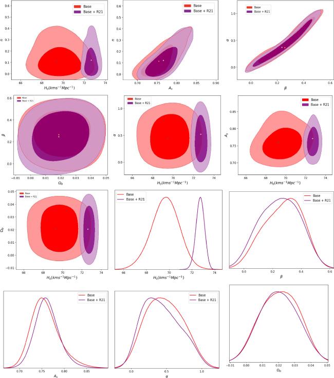
Figure 2. 2D contours at 68.3% and 95.4% confidence levels for pairs (n, H0), (n, As), (α, β), (β, Ωb), (α, H0), (As, H0) and (Ωb, H0), and 1D posterior distribution of H0, β, As, α and Ωb for the VGCG model with matter creation using BASE and BASE+R21 datasets, repsectively. |

Figure 3. 2D contour at 68.3% and 95.4% confidence levels for pairs (β, H0), (As, H0), (β, As), (As, Ωb), (Ωb, H0), (n, H0), (n, As) and (β, Ωb), and 1D posterior distribution of H0, As, β and Ωb for the VCG model with matter creation using BASE and BASE+R21 datasets. |
Table 2. The constraints on the parameters of VGCG and VCG models without matter creation. The combined dataset of BAO + CC + SC is referred to as ‘BASE'. |
| Model | Parameters | BASE | BASE + R21 |
|---|---|---|---|
| H0 [kms−1Mpc−1] | ${69.674}_{-0.563}^{+1.217}$ | ${72.670}_{-0.412}^{+1.326}$ | |
| Ωb | ${0.020}_{-0.024}^{+0.015}$ | ${0.020}_{-0.015}^{+0.014}$ | |
| VGCG | As | ${0.767}_{-0.033}^{+0.012}$ | ${0.770}_{-0.016}^{+0.021}$ |
| n | ${0.129}_{-0.026}^{+0.101}$ | ${0.116}_{-0.011}^{+0.004}$ | |
| α | ${0.040}_{-0.017}^{+0.021}$ | ${0.042}_{-0.061}^{+0.072}$ | |
| | |||
| H0 [kms−1Mpc−1] | ${69.870}_{-0.365}^{+1.133}$ | ${72.640}_{-0.352}^{+1.362}$ | |
| Ωb | ${0.030}_{-0.036}^{+0.025}$ | ${0.030}_{-0.021}^{+0.005}$ | |
| VCG | As | ${0.994}_{-0.002}^{+0.001}$ | ${0.994}_{-0.021}^{+0.017}$ |
| n | ${1.140}_{-0.101}^{+0.032}$ | ${0.128}_{-0.035}^{+0.041}$ | |
In what follows, we discuss the evolutions of different cosmological parameters, the stability of the models, selection criteria and Bayesian evidence analysis to compare the proposed models with the existing dark energy models.
7.1. Evolution of cosmological parameters
The evolutions of H(z) with respect to the redshift z for VGCG and VCG models with and without matter creation are shown in figures 4–7. The figures also show a comparison of VGCG and VCG models with the ΛCDM model. As observed, the VCG model closely matches the observed data during the whole evolution, whereas the VGCG model coincides during the late-time evolution of the Universe.

Figure 4. Evolution of H(z) with redshift z in VGCG and VCG models with matter creation, and the ΛCDM model using the BASE dataset. The grey points with uncertainty bars corresponds to the H(z) sample. The black bold line represents the ΛCDM model. |

Figure 5. Evolution of H(z) with redshift z in VGCG and VCG models with matter creation, and the ΛCDM model using the BASE+R21 dataset. The grey points with uncertainty bars corresponds to the H(z) sample. The black bold line represents the ΛCDM model. |

Figure 6. Evolution of H(z) with redshift z in VGCG and VCG models without matter creation, and the ΛCDM model using the BASE dataset. The grey points with uncertainty bars corresponds to the H(z) sample. The black bold line represents the ΛCDM model. |

Figure 7. Evolution of H(z) with redshift z in VGCG and VCG models without matter creation, and the ΛCDM model using the BASE+R21 dataset. The grey points with uncertainty bars corresponds to the H(z) sample. The black bold line represents the ΛCDM model. |
Using BASE and BASE + R21 datasets, we obtain the present values of q(z), w(z) and j(z) for ΛCDM, VGCG and VCG models with and without matter creation, which are summarized in tables 3 and 4. The evolutions of q(z) with redshift z of all three models for BASE and BASE + R21 datasets are shown in figures 8 and 9, respectively. We observe that the models show a transition from deceleration (q(z) > 0) to acceleration (q(z) < 0). In figures, a dot represents the present value of q(z). The present values of q(z) at z = 0 from BASE and BASE + R21 datasets are ${q}_{0}=-{0.591}_{-0.01}^{+0.01}$ and ${q}_{0}=-{0.590}_{-0.02}^{+0.02}$ for the ΛCDM model, ${q}_{0}=-{0.541}_{-0.02}^{+0.02}$ and ${q}_{0}=-{0.542}_{-0.05}^{+0.05}$ for the VGCG model and ${q}_{0}\,=-{0.553}_{-0.03}^{+0.03}$ and ${q}_{0}=-{0.555}_{-0.03}^{+0.03}$ for the VCG model with matter creation, respectively, as given in table 3. The values of q0 show that the models undergo accelerated expansion at present-day. We obtain the transition value ztr where the models transit from deceleration to acceleration at ${z}_{{tr}}\,={0.610}_{-0.022}^{+0.030}$ and ${z}_{{tr}}={0.631}_{-0.023}^{+0.037}$ for the VGCG model, and ${z}_{{tr}}={0.674}_{-0.016}^{+0.029}$ and ${z}_{{tr}}={0.687}_{-0.031}^{+0.036}$ in the case of the VCG model, respectively. These transition values are very close to the ΛCDM transition values (see table 3). We also present the values of ztr and q0 in table 4 for these models without matter creation.

Figure 8. Evolution of q(z) with z in VGCG and VCG models with matter creation, and the ΛCDM model using the BASE dataset. The dots represent the present value of q(z). |

Figure 9. Evolution of q(z) with z in VGCG and VCG models with matter creation, and the ΛCDM model using the BASE+R21 dataset. The dots represent the present value of q(z). |
Table 3. The present values of different cosmological and geometrical parameters of ΛCDM, VGCG and VCG models with matter creation. |
| Models → | ΛCDM | VGCG | VCG | |||
|---|---|---|---|---|---|---|
| Parametrs | BASE | +R21 | BASE | +R21 | BASE | +R21 |
| ztr | ${0.692}_{-0.029}^{+0.034}$ | ${0.689}_{-0.033}^{+0.028}$ | ${0.610}_{-0.022}^{+0.030}$ | ${0.631}_{-0.023}^{+0.037}$ | ${0.674}_{-0.016}^{+0.029}$ | ${0.687}_{-0.031}^{+0.036}$ |
| q0 | $-{0.591}_{-0.01}^{+0.01}$ | $-{0.590}_{-0.02}^{+0.02}$ | $-{0.541}_{-0.02}^{+0.02}$ | $-{0.542}_{-0.05}^{+0.05}$ | $-{0.553}_{-0.03}^{+0.03}$ | $-{0.555}_{-0.03}^{+0.03}$ |
| w0 | $-{0.726}_{-0.04}^{+0.04}$ | $-{0.728}_{-0.01}^{+0.01}$ | $-{0.730}_{-0.11}^{+0.11}$ | $-{0.740}_{-0.13}^{+0.13}$ | $-{0.721}_{-0.02}^{+0.02}$ | $-{0.728}_{-0.02}^{+0.02}$ |
| t0 (Gyr) | ${13.73}_{-0.02}^{+0.02}$ | ${13.76}_{-0.04}^{+0.04}$ | ${13.91}_{-0.03}^{+0.03}$ | ${13.94}_{-0.07}^{+0.07}$ | ${13.87}_{-0.03}^{+0.03}$ | ${13.89}_{-0.01}^{+0.01}$ |
| j0 | 1 | 1 | ${0.933}_{-0.21}^{+0.21}$ | ${0.941}_{-0.10}^{+0.10}$ | ${0.979}_{-0.02}^{+0.02}$ | ${0.966}_{-0.02}^{+0.02}$ |
| ${C}_{s}^{2}$ | — | — | 0.329 | 0.379 | 0.730 | 0.740 |
Table 4. The present values of different cosmological and geometrical parameters of VGCG and VCG models without matter creation. |
| Models → | VGCG | VCG | ||
|---|---|---|---|---|
| Parametrs | BASE | +R21 | BASE | +R21 |
| ztr | ${0.689}_{-0.021}^{+0.023}$ | ${0.694}_{-0.024}^{+0.019}$ | ${0.955}_{-0.023}^{+0.018}$ | ${0.922}_{-0.014}^{+0.018}$ |
| q0 | $-{0.652}_{-0.02}^{+0.02}$ | $-{0.617}_{-0.02}^{+0.02}$ | $-{0.590}_{-0.02}^{+0.02}$ | $-{0.573}_{-0.02}^{+0.02}$ |
| w0 | $-{0.589}_{-0.11}^{+0.11}$ | $-{0.595}_{-0.15}^{+0.15}$ | $-{0.838}_{-0.01}^{+0.01}$ | $-{0.842}_{-0.02}^{+0.02}$ |
| t0 (Gyr) | ${13.77}_{-0.01}^{+0.01}$ | ${13.83}_{-0.03}^{+0.03}$ | ${13.91}_{-0.02}^{+0.02}$ | ${13.93}_{-0.01}^{+0.01}$ |
| j0 | ${0.959}_{-0.19}^{+0.19}$ | ${0.742}_{-0.21}^{+0.21}$ | ${0.892}_{-0.11}^{+0.11}$ | ${1.01}_{-0.12}^{+0.12}$ |
| ${C}_{s}^{2}$ | 0.414 | 0.490 | 0.781 | 0.805 |
The evolutions of the EoS parameter w(z) with z of ΛCDM, VGCG and VCG models are shown in figures 10 and 11 with two datasets. For both datasets, the EoS shows a quintessence phase (−1 < w < 0) at present and ΛCDM behavior at a late epoch. Figures 12 and 13 show the evolutions of the jerk parameter j(z) with respect to z for the discussed models using BASE and BASE + R21 datasets. Based on these two datasets, the present values of j(z) for the VGCG model are ${j}_{0}={0.933}_{-0.21}^{+0.21}$ and ${j}_{0}={0.941}_{-0.10}^{+0.10}$, whereas for the VCG model we obtain ${j}_{o}={0.979}_{-0.02}^{+0.02}$ and ${j}_{0}\,={0.966}_{-0.02}^{+0.02}$, respectively, which are very close to the value j0 = 1 of the ΛCDM model.
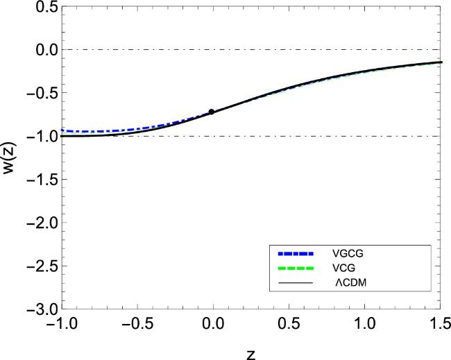
Figure 10. Evolution of w(z) with z in VGCG and VCG models with matter creation, and the ΛCDM model using the BASE dataset. The dots represent the present value of w(z). |
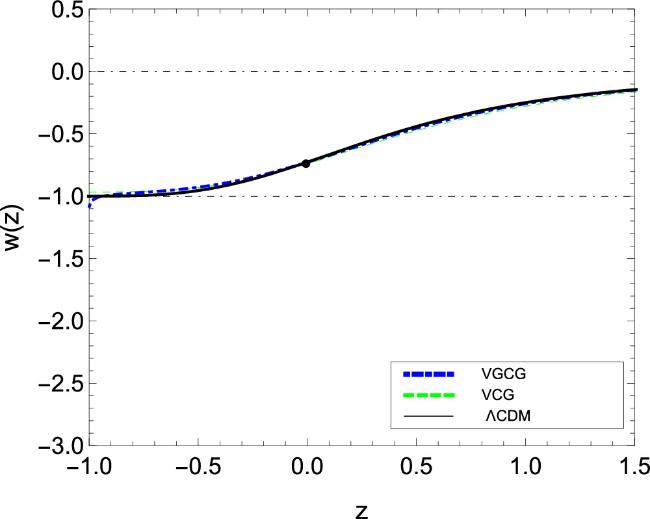
Figure 11. Evolution of w(z) with z in VGCG and VCG models with matter creation, and the ΛCDM model using the BASE+R21 dataset. The dots represent the present value of w(z). |
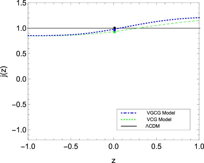
Figure 12. Trajectories of j(z) for VGCG and VCG models with matter creation, and the ΛCDM model using best-fit values from the BASE dataset. The dots represent the present value of j0. |
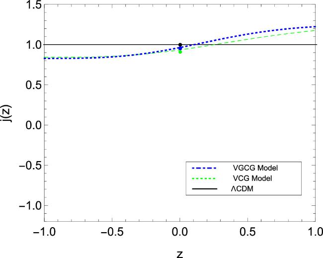
Figure 13. Trajectories of j(z) for VGCG and VCG models with matter creation, and the ΛCDM model using the BASE+R21 datasets The dots represent the present value of j0. |
The ages of the Universe for all the models are given in table 3. The constrains on the age of the Universe for the VGCG model are ${t}_{0}={13.91}_{-0.03}^{+0.03}$ Gyr with the BASE dataset and ${t}_{0}={13.94}_{-0.07}^{+0.07}$ Gyr with the BASE + R21 dataset, whereas for the VCG model we have ${t}_{0}={13.87}_{-0.03}^{+0.03}$ Gyr and ${t}_{0}={13.89}_{-0.01}^{+0.01}$ Gyr, respectively. The ages of the Universe for these CG models are very close to the age of the Universe for the ΛCDM model. In table 4, we list the present values of ztr, q0, w0, j0 and t0 for the proposed models without matter creation to compare the deviation for constraint results on extended CG models with matter creation.
7.2. Stability of the model
In order to determine the stability of the models, we analyze the squared sound speed of the VGCG and VCG fluids with and without matter creation. For any cosmic fluid model, the squared sound speed ${{ \mathcal C }}_{S}^{2}$ can be estimated from the relation: ${{ \mathcal C }}_{S}^{2}={{dp}}_{{Ch}}/{\rm{d}}{\rho }_{{Ch}}$. It is noted that ${{ \mathcal C }}_{S}^{2}\geqslant 0$ corresponds to stable behavio,r while ${{ \mathcal C }}_{S}^{2}\lt 0$ leads to unstable behavior of the model. Thus, the physical values of ${{ \mathcal C }}_{s}^{2}$ for a stable model must be in the range of (0, 1). Outside of this region, one encounters gradient/tachyonic instabilities and/or instabilities linked to superluminal propagation.
The squared sound speed for the VGCG model is given by
$\begin{eqnarray}{{ \mathcal C }}_{S}^{2}=\displaystyle \frac{\alpha {A}_{s}\left(1-\tfrac{n}{3(1-\beta )(1+\alpha )}\right){\left(1+z\right)}^{n}}{{A}_{s}{\left(1+z\right)}^{n}+(1-{A}_{s}){\left(1+z\right)}^{3(1-\beta )(1+\alpha )}}.\end{eqnarray}$
and for VCG model, we have $\begin{eqnarray}{{ \mathcal C }}_{S}^{2}=\displaystyle \frac{{A}_{s}\left(1-\tfrac{n}{6(1-\beta )}\right){\left(1+z\right)}^{n}}{{A}_{s}{\left(1+z\right)}^{n}+(1-{A}_{s}){\left(1+z\right)}^{6(1-\beta )}}.\end{eqnarray}$
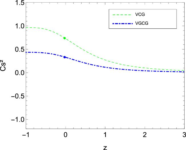
The sound speed should be positive in the stable model and, hence, this is justified by taking the constant α > 0. Using the best-fit values of model parameters from the BASE and BASE+R21 datasets in the above equations, we find the current values ${{ \mathcal C }}_{S}^{2}=0.329$ and ${{ \mathcal C }}_{S}^{2}=0.379$ for the VGCG model, and ${{ \mathcal C }}_{S}^{2}=0.730$ and ${{ \mathcal C }}_{S}^{2}=0.740$ for VCG model, which are listed in table 3. We plot the trajectories of ${{ \mathcal C }}_{S}^{2}$ with z in figures 14 and 15 using two combinations of datasets for VGCG and VCG models. The trajectories show that the squared sound speed is always positive throughout the evolution lying in the range (0, 1) and, hence, positive and less than unity in both the discussed models. This ensures that these models do not surpass the velocity of light, which confirms their stability. Table 4 shows ${{ \mathcal C }}_{S}^{2}$ for VGCG and VCG models without matter creation. The ${{ \mathcal C }}_{S}^{2}$ values are positive and less than unity, which also confirms the stability.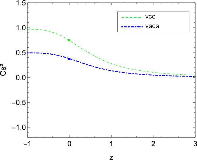
Figure 14. Trajectories of ${{ \mathcal C }}_{s}^{2}$ for VGCG and VCG models with matter creation using best-fit values of the BASE dataset. |
Figure 15. Trajectories of ${{ \mathcal C }}_{s}^{2}$ for VGCG and VCG models with matter creation using best-fit values of the BASE+R21 dataset. |
7.3. Model selection
We calculate the values of ${\chi }_{\min }^{2}/{dof}$ for ΛCDM, VGCG and VCG models with and without matter creation, shown in tables 5 and 6, respectively. Here, the value of dof (degree of freedom) equals the number of observational data points (N) minus the number of parameters (K). The number of observational data points for the BASE dataset is N = 273 (CC = 30, type Ia supernova (Pantheon) = 40, uncorrelated BAO = 17, Hubble diagram for quasars = 24 and gamma-ray bursts = 162), and N = 274 for the BASE+R21 dataset, and the number of parameters are K = 3, 6 and 5 for ΛCDM, VGCG and VCG models with matter creation, and K = 5 and 4 for VGCG and VCG models without matter creation, respectively. From tables 5 and 6, we observe that both the models with and without matter creation have ${\chi }_{\min }^{2}/{dof}\lt 1$ for both datasets. This shows that both the models are in good agreement with respect to the observational data as far as ${\chi }_{\min }^{2}/{dof}$ is concerned.
Table 5. ${\chi }_{{red}}^{2}$, AIC (BIC), Bayesian evidence and Bayes factor values for ΛCDM, VGCG and VCG models with matter creation. Here the ΛCDM model is taken as a reference model to calculate ΔAIC, ΔBIC and $\mathrm{ln}B$. |
| Model | Parameters | BASE | +R21 |
|---|---|---|---|
| ${\chi }_{\min }^{2}$ | 253.92 | 254.17 | |
| ${\chi }_{\min }^{2}/{dof}$ | 0.94 | 0.94 | |
| ΛCDM | AIC | 260.01 | 260.26 |
| BIC | 270.75 | 271.00 | |
| $\mathrm{ln}E(M1)$ | −123.824 | −124.116 | |
| | |||
| ${\chi }_{\min }^{2}$ | 255.51 | 257.74 | |
| ${\chi }_{\min }^{2}/{dof}$ | 0.965 | 0.953 | |
| AIC | 267.82 | 270.05 | |
| VGCG | BIC | 289.16 | 291.41 |
| ΔAIC | 7.81 | 9.79 | |
| ΔBIC | 18.41 | 20.41 | |
| $\mathrm{ln}\ E(M2)$ | −125.938 | -126.099 | |
| lnB12 | 2.114 | 1.983 | |
| Evidence interpretation | positive | positive | |
| | |||
| ${\chi }_{\min }^{2}$ | 254.59 | 257.63 | |
| ${\chi }_{\min }^{2}/{dof}$ | 0.95 | 0.96 | |
| AIC | 264.81 | 267.86 | |
| VCG | BIC | 282.64 | 285.70 |
| ΔAIC | 4.80 | 7.60 | |
| ΔBIC | 11.89 | 14.70 | |
| $\mathrm{ln}E(M2)$ | −126.513 | −126.697 | |
| lnB12 | 2.689 | 2.581 | |
| Evidence interpretation | moderate | moderate | |
Table 6. ${\chi }_{{red}}^{2}$, AIC (BIC), Bayesian evidence and Bayes factor values for VGCG and VCG models without matter creation. Here, the ΛCDM model is taken as a reference model to calculate ΔAIC, ΔBIC and $\mathrm{ln}B$. |
| Model | Parameters | BASE | +R21 |
|---|---|---|---|
| ${\chi }_{\min }^{2}$ | 255.32 | 257.94 | |
| ${\chi }_{\min }^{2}/{dof}$ | 0.956 | 0.962 | |
| AIC | 265.54 | 268.16 | |
| VGCG | BIC | 283.36 | 286.01 |
| ΔAIC | 5.53 | 7.92 | |
| ΔBIC | 12.61 | 15.01 | |
| $\mathrm{ln}E(M2)$ | −126.095 | −125.486 | |
| lnB12 | 2.271 | 1.370 | |
| Evidence interpretation | Positive | Positive | |
| | |||
| ${\chi }_{\min }^{2}$ | 254.21 | 255.76 | |
| ${\chi }_{\min }^{2}/{dof}$ | 0.959 | 0.950 | |
| AIC | 262.36 | 263.91 | |
| VCG | BIC | 276.65 | 278.21 |
| ΔAIC | 2.35 | 3.67 | |
| ΔBIC | 5.90 | 7.21 | |
| $\mathrm{ln}E(M2)$ | −132.818 | −132.434 | |
| lnB12 | 8.994 | 8.318 | |
| Evidence interpretation | Decisive | Decisive | |
Although the above analyses are in good agreement with one another, further differences arise due to the choice of cosmological model made.
In what follows, we use the information criteria (IC), which have a deep underpinning in the theory of statistical inference. There are two such IC, namely, Akaike information criteria (AIC) [87] and Bayesian information criteria (BIC) [88], which are, respectively, defined as
$\begin{eqnarray}{AIC}={\chi }_{\min }^{2}+\displaystyle \frac{2{NK}}{N-K-1},\end{eqnarray}$
$\begin{eqnarray}{BIC}={\chi }_{\min }^{2}+K\mathrm{ln}N,\end{eqnarray}$
where ${\chi }_{\min }^{2}$ measures the quality of the model and K, the number of parameters, indicates model complexity. We calculate the relative values between different models. The one that minimizes the AIC (or BIC) is usually considered the best model. Using the ΛCDM as the reference model, we define the AIC and BIC differences as follows: ΔAIC = AICx −AICΛCDM and ΔBIC = BICx −BICΛCDM, where x represents either the VGCG or the VCG model. This gives the assessment of the strength of the models. The criteria for judging the AIC model [89] are as follows: when 0 ≤ ΔAIC < 2, the model has almost the same support from the data as the best model; for 2 < ΔAIC ≤ 4, the model is considerably less supported; and the range 4 < ΔAIC < 10 still supports the considered model. The observational data do not support the model at values of ΔAIC > 10.In the case of BIC, the range ΔBIC < 2 is considered to support the model from observational data. There is slight evidence against the considered model if 2 < ΔBIC < 6. For a value in the range 6 < ΔBIC < 10, we obtain strong evidence against the considered model; if ΔBIC > 10, we obtain even stronger evidence against the model [90].
The AIC (BIC) and ΔAIC(ΔBIC) for VGCG and VCG models with and without matter creation against the ΛCDM model are listed in tables 5 and 6, respectively. The ΔAIC values of VGCG and VCG models show that these models are still supported by current observational data. For the BIC selection method, it seems that these models are not favored by observational data. The reason is that AIC is always more general towards extra parameters, whereas BIC tends to penalize them. Hence, the AIC remains useful as it gives an upper limit to the number of parameters.
7.4. Bayesian evidence analysis
In this subsection, we first briefly review the basis of Bayesian inference and model comparison. We then present the computation of the Bayes factor of the two proposed models. The Bayesian evidence applies the same type of likelihood analysis familiar from parameter estimation, but at the level of models rather than parameters. It depends on goodness of fit across the entire model parameter space [91]. It comes from a full implementation of Bayesian inference at the model level, and is the probability of the data given the model. It updates the prior model probability to the posterior model probability using Bayes theorem. The Bayesian evidence is defined as [91–93]
$\begin{eqnarray}E=\int { \mathcal L }(\theta )P(\theta )\,{\rm{d}}\theta ,\end{eqnarray}$
where θ is the vector of parameters, ${ \mathcal L }$ is the likelihood and P(θ) is the prior distribution of those parameters before the data were obtained. The evidence of a model is thus the average likelihood of the model in the prior. The Bayesian evidence rewards model predictiveness. Hence, the evidence will not penalize the extra parameter in this case, because it does not change the model parameters.The ratio of the evidence of two models, say M1 and M2, is known as the Bayes factor, which is defined as [94]6 . We assumed the ΛCDM model as the reference one, say M1, and, therefore, its entry is zero by definition.
$\begin{eqnarray}{B}_{12}=\displaystyle \frac{E({M}_{1})}{E({M}_{2})}.\end{eqnarray}$
The Bayes factor provides a measure with which to discriminate between the models. It is usual to consider the logarithm of the Bayes factor, for which the so-called Jeffreys scale [95, 96] gives empirically calibrated levels of significance for the strength of evidence. Many papers on Bayesian evidence have adopted the interpretive scale suggested by Jeffreys, which is presented in table 7. For each model and dataset we estimate the values of the logarithm of the Bayesian evidence ($\mathrm{ln}E$) and the Bayes factor ($\mathrm{ln}B$), which is the difference between the mean $\mathrm{ln}E$ of the ΛCDM model and the model concerned. These values are obtained by taking the priors and the dataset described in section Table 7. Jeffrey' Interpretive scales for the strength of evidence when comparing two models, M1 and M2. |
| lnB12 | Strength of evidence |
|---|---|
| <1 | Inconclusive |
| 1.0 − 2.5 | Positive evidence |
| 2.5 − 5.0 | Moderate evidence |
| >5 | Decisive |
Table 5 presents the Bayesian evidence and Bayes factor for VGCG and VCG models with matter creation. Looking at the BASE and BASE+R21 datasets, respectively, we find $\mathrm{ln}{B}_{12}=2.114$ and $\mathrm{ln}{B}_{12}=1.983$ for the VGCG model, and $\mathrm{ln}{B}_{12}=2.689$ and $\mathrm{ln}{B}_{12}=2.581$ for the VCG model, which suggest that the VGCG model has positive evidence, while the VCG model has moderate evidence.
Similarly, using the priors and the same datasets, we obtain the Bayes factor for VGCG and VCG models without matter creation, which are provided in table 6. By considering the BASE data, we find $\mathrm{ln}{B}_{12}=2.271$ for the VGCG model and $\mathrm{ln}{B}_{12}=8.994$ for the VCG model. The BASE+R21 data give $\mathrm{ln}{B}_{12}=1.37$ for the VGCG model and $\mathrm{ln}{B}_{12}=8.318$ for the VCG model. This suggests that the VGCG model has positive evidence from both the datasets, whereas the VCG model has strong (decisive) evidence.
8. Conclusion
In this paper, we have examined the VGCG model inspired by the matter creation mechanism in cosmology. Our motivation for this study was to investigate the effects of matter creation on the evolution of the Universe filled by VGCG as a perfect fluid using the latest cosmological observations. In particular we have proposed two CG models with matter creation, i.e., VGCG and VCG and have investigated their evolutionary behaviors via observational datasets. We have placed constraints on them using two different data combinations: BASE (BAO+CC+SC) and BASE+R21. We have found that the VGCG, VCG and ΛCDM models give a similar ${\chi }_{\min }^{2}$ and, correspondingly, ${\chi }_{\min }^{2}/{dof}$. In what follows, we summarize the results and evolutions of these models.
As stated above, the focus has been on exploring the cosmological models influenced by gravitational matter creation, specifically considering an extended version of the CG with EoS ${p}_{{Ch}}=-\tfrac{A(a)}{{\rho }_{{Ch}}^{\alpha }}$ where 0 < α ≤ 1. This approach is utilized to examine the late-stage acceleration of the Universe within the context of a flat FLRW space-time. Additionally, we have delved into a special scenario where α = 1, corresponding to the VCG with EoS ${p}_{{Ch}}=-\tfrac{A(a)}{{\rho }_{{Ch}}}$, and incorporated the concept of matter creation. A parallel discussion on these models without matter creation has also been presented.
In the preliminary discussion, it has been explained that matter creation induced by gravity can be regarded as an irreversible scalar phenomenon, contributing an extra decay (or creation) pressure to the energy–momentum tensor in the cosmological fluid mixture. This supplementary creation pressure is characterized by the matter creation rate, denoted as Γ, along with other relevant physical parameters of the fluid. Studies have shown that viewing the Universe as an open system with ongoing matter creation aids in comprehending its current rapid expansion phase. As the nature of the matter creation rate Γ is still unknown, we have adopted a phenomenological approach, assuming Γ evolves as Γ ∝ H. These models were found to be consistently either decelerating or accelerating, lacking a transition from a deceleration phase to an acceleration phase, contradicting the SNe observational data. Nevertheless, our findings indicate that by incorporating the VGCG and VCG equations of state in the matter creation model, a phase transition does occur, even with the aforementioned form of Γ.
The initial section of this manuscript details the analytical solutions derived for matter creation models applying both VGCG and VCG equations of state. Solutions for various cosmological parameters such as energy density, Hubble parameter, deceleration parameter, EoS parameter and jerk parameter have been deduced as functions of redshift. In the manuscript's latter section, two different joint observational analyses have been performed to constrain the parameters of the model. Tables 1 and 2 present the best-fit values for these model parameters with and without matter creation. We observe that VGCG and VCG models with matter creation can alleviate the current H0 tension from 3.92σ to 1.51σ and 1.84σ using the BASE data. The current values for q(z), j(z), w(z), t(z) and ${{ \mathcal C }}_{S}^{2}$ are listed in tables 3 and 4 and their evolutions have been plotted in figures 4–13. Our observations indicate a notable variance in the VGCG and VCG models with parameter β from the ΛCDM model. These plots vividly illustrate the models' capability to generate late-stage cosmic acceleration while also reflecting a decelerated expansion in earlier times. The transition redshift values, q0, w0 and age of the Universe with respect to VGCG and VCG models with and without matter creation are found to be very close to the ΛCDM model and the Planck 2018 release. The evolution trajectories of j(z) reveal minimal deviation from the ΛCDM model for both VGCG and VCG models.
he AIC and BIC analysis show that models such as VGCG and VCG with and without matter creation exhibit in the range of 4 < ΔAIC < 10, suggesting to as much as the preferred model with the joint observational data. In terms of BIC values, the models VGCG and VCG with and without matter creation present ΔBIC > 10, providing evidence against the data used for analysis. It is noteworthy that the squared sound speed for these models lies within the $0\lt {{ \mathcal C }}_{S}^{2}\lt 1$ range, thereby not exceeding the speed of light, which signifies the stability of these models. Consequently, it is deduced that the models discussed in this paper yield cosmological parameters that are well bounded by the combined observational data. Furthermore, these models closely resemble the ΛCDM model in their behavior.
In statistical sense, a physical model may be thought of as described by a set of parameters. The determination of these parameters may be carried out in many ways: the most commonly used framework to accomplish this is Bayesian evidence analysis. We have calculated the Bayesian evidence and, consequently, the Bayes factor to measure the discrimination between the models. Assuming priors for different parameters and the ΛCDM model as the reference one, we have found that the VGCG model with and without matter creation has positive evidence on the Jeffrey scale, whereas the VCG model has moderate evidence with matter creation, and has decisive evidence without matter creation by both datasets.