


1. Introduction
Pulsar emissions are generated within celestial bodies like neutron stars through enhanced rotation, which is influenced by the rotational force, known as the Coriolis force [1]. In the study of ionized media, the presence of the Coriolis force gives rise to magnetic-field-like effects that significantly impact wave phenomena. The dynamics of such plasma systems are best understood when analyzed in non-inertial frames, and these theoretical frameworks have been successfully applied to investigate plasma dynamics in both laboratory and astrophysical contexts [2]. Notably, the application of non-inertial frames has proved to be a useful tool in the study of narrow wave packets, such as pulsar radiation, when the Coriolis force is present [3]. Mushtaq and Shah [4] examined the characteristics of two-dimensional obliquely propagating ion acoustic waves (IAWs) in spinning, relativistic magnetised electron-positron-ion (e-p-i) plasmas have been studied, and the phase velocity is found to be inversely proportional to the positron concentration. It has been observed that as the rates of rotation and the frequencies associated with the motion of charged particles in a magnetic field increase, the breadth of solitary waves associated with these waves decreases. This suggests that the connection between rotation and the external magnetic field amplifies the spiky characteristics of the solitary structures.
In dense plasma (quantum) systems found in astrophysical objects, the de Broglie wavelength linked with fermions becomes similar to the interparticle distance, and the Fermi temperature surpasses the system temperature due to the overlapping of wave functions. In such conditions, the plasma system exhibits quantum mechanical effects, which cannot be ignored. The system also obeys the Fermi–Dirac distribution rather than the Maxwell–Boltzmann distribution. Electrostatic and electromagnetic plasma waves in dense plasma systems have been explored using the quantum hydrodynamic model by taking into account different quantum effects, such as quantum statistical, Bohm Potential and spin effects. It has been established that the characteristics of plasma waves in dense plasmas are different from those in classical plasmas [5–9]. The effects of the Coriolis force may play an essential part in the study of rotating astronomical objects with compact (dense) plasmas [10, 11].
When a significant ambient magnetic field is present, the typical energy associated with electron cyclotron motion exceeds the Coulomb energy, leading to qualitative alterations in the properties of atoms [12]. Landau diamagnetism or Landau quantization occurs when orbital motion of degenerate fermions is quantized under the sway of a magnetic field [13]. This quantization of a magnetic field affects the equation of state of fermions in fully degenerate and partially degenerate plasmas [14]. The characteristics of longitudinal waves in quantum plasma with the effects of Landau diamagnetism were studied, and it was demonstrated that the dispersion relation of the longitudinal wave traveling along a magnetic field is highly dependent on the strength of the magnetic field [15]. Subsequent investigations have further explored the oblique propagation of IAWs in quantized magnetic fields, revealing that only compressive solitary structures excite in this scenario. The interplay between the magnetic-field quantization and the plasma degeneracy significantly influences the dynamics of IAWs and gives rise to intriguing solitary wave structures [16]. Later studies explored the fact that the oblique propagation of IAWs in a quantized magnetic field results in only compressive solitary structures [17].
Electron–positron (e-p) plasmas are frequently encountered in diverse astrophysical settings, including the early Universe, pulsars, supernova remnants, active galactic nuclei, γ-ray bursts and the central region of the Milky Way galaxy. [18]. Positrons are used for a variety of studies, for example, in the characterization of materials and surfaces, plasma physics and anti-hydrogen formation [19]. Positrons are also created in laboratory experiments for different applications [20]. Nonlinear formations, such as solitons, shock waves and double layers, have been investigated in classical and quantum plasmas. Ion acoustic (IA) solitons in classical e-p-i plasma have been researched, revealing a decrease in the amplitude of the solitary structure when positrons are present [21]. Also, El-Labany et al explored the characteristics of nonlinear Langmuir patterns in a mildly relativistic e-p magnetoplasma with immobile positive ions affected by rotation. They utilized both theoretical and numerical methods to analyze the behavior of these patterns within the plasma system [22]. The formation of IA shocks in e-p-i rotating Lorentzian plasmas have revealed the fact that the changes in the concentration of positrons are responsible for the shift of the distribution function [23]. In dense plasmas, the effects of Landau quantization, when positrons are present, have been investigated. It has been noted that the phase velocity of the IASWs diminishes as a result of the influence of Landau quantization effects in e-p-i plasmas [24].
The effects of ion–neutral collisions in the presence of positrons and Landau quantization have been investigated in non-inertial frames. Sahu et al [25] examined electrostatic nonlinear structures in rotating quantum plasmas. They examined IAWs propagating at an angle in a magnetized quantum plasma, affected by rotation within an external magnetic field. The research revealed that as quantum effects strengthen and rotational speeds increase, the solitary waves become more tightly bound, resulting in energy dissipation. Weakly dissipative solitons in ion–neutral collisions in quantum plasmas were also studied, resulting in the excitation of hump-shaped solitary structures [26]. Similarly, in pair-ion plasmas, weakly dissipative hump and dip solitons were observed when collisions were present [27]. The behavior of weak dissipative IASWs in relativistic degenerate plasmas under the influence of collisions was also investigated, revealing a decrease in soliton energy over time in the presence of the collision term [28].
The Kawahara equation (KE) is a fifth-order Korteweg–de Vries (fKdV) equation that takes into account the higher-order dispersion effects and provides a more accurate description of nonlinear waves in certain scenarios. The KE has been successfully used to study wave dynamics in various physical systems, such as waves in water, waves in plasma and optical solitons. The KE incorporates a fifth-order dispersion term that serves to balance the nonlinearity of the wave equation. This delicate balance allows the accurate representation of wave propagation, particularly in scenarios where the dispersion coefficient is small or approaches zero. This is particularly important in laboratory experiments, where the small dispersion coefficient can significantly affect the behavior of nonlinear waves [29]. By considering the KE, researchers can obtain a more comprehensive understanding of wave phenomena and accurately predict their characteristics. Recently, the investigation of damped Kawahara IASWs and cnoidal waves (CWs) in a degenerate magneto-rotating plasma has been conducted in e-i plasmas [30]. The ions are considered to be classical particles, while the electrons follow the Fermi–Dirac distribution. The author considered the collisions as well as the Coriolis force effect. The author derived the damped KE, which is a fully non-integrable differential equation. The estimated solution of the equation has indicated that as the quantizing parameter increases, both the amplitude and width of the damped Kawahara solitons' solitary structures also increase.
The aim of this study is to examine the characteristics and behavior of IA damped Kawahara waves in a collision plasma comprising three unique species of electrons, positrons and ions. The plasma is subjected to an externally applied magnetic field $\vec{B}={B}_{0}\hat{z}$, which is uniformly directed along the z-axis. Furthermore, the plasma is considered to rotate with an angular frequency Ω at an angle θ relative to the magnetic-field direction. It should be noted that the rotation is thought to be on a lower scale than the ion gyrofrequency. The influence of various plasma characteristics on the forms of linear and nonlinear waves in an e-p-i plasma will be investigated. We will specifically look at how changes in parameters like Landau quantization, the direction cosine, the normalized positron-to-electron density ratio, the normalized positron-to-ion density ratio, the rotational frequency, the inclination angle and magnetic-field strength affect the properties of these waves. To acquire a thorough understanding of the system, both linear and nonlinear wave phenomena will be investigated.
This paper is structured as follows: section 2 presents the basic nonlinear governing equations of the system under consideration. In section 3 , linear analysis of the system is performed, and the dispersion relation for the linear waves is derived. Section 4 uses the reductive perturbation approach to investigate small-amplitude nonlinear systems under the assumption of slow rotation. Section 5 delves into the semi-analytic solution of the damped Kawahara problem. Sections 4 and 5 present plots illustrating the effects of various plasma properties on plasma waves. Finally, section 6 summarizes the study's principal findings.
2. Fundamental set of equations
In the context of studying a three component e-p-i dense, homogeneous, magnetized and collisional plasma, we utilize an assumption that the plasma is undergoing slow rotation due to the Coriolis force. This rotation occurs with an angular frequency Ω around an axis specified in the xz-plane, forming an angle θ. Mathematically, we can express this angular frequency as ${\boldsymbol{\Omega }}=({{\rm{\Omega }}}_{0x}\hat{x},0,{{\rm{\Omega }}}_{0z}\hat{{\rm{z}}})$, where ${{\rm{\Omega }}}_{0x}={{\rm{\Omega }}}_{0}\cos \theta $ and ${{\rm{\Omega }}}_{0z}={{\rm{\Omega }}}_{0}\sin \theta $. We focus on the ions, which are assumed to be cold and non-degenerate because of their heavier mass than that of the electrons and positrons. To analyze the behavior of classical ions in the rotating frame of reference, we consider the continuity and momentum governing equations. These equations describe the conservation of mass and momentum for the ions, accounting for the effects of the rotating frame,2 ) results from the rotation of the plasma at an angle of approximately Ω, which causes Coriolis force effects. Quadratic and higher-order terms, like centrifugal force ∼Ω × (Ω × r), can safely be ignored if rotation is assumed to be sluggish. Here, ν is the collisions of ions with the neutrals.
$\begin{eqnarray}\displaystyle \frac{\partial {n}_{i}}{\partial t}+{\boldsymbol{\nabla }}.\left({n}_{i}{{\boldsymbol{v}}}_{i}\right)=0,\end{eqnarray}$
$\begin{eqnarray}\begin{array}{l}{m}_{i}\left(\displaystyle \frac{\partial {{\boldsymbol{v}}}_{i}}{\partial t}+({{\boldsymbol{v}}}_{i}.{\boldsymbol{\nabla }}){{\boldsymbol{v}}}_{i}\right)=e{\boldsymbol{E}}+\displaystyle \frac{e}{c}({{\boldsymbol{v}}}_{i}\times {\boldsymbol{B}})\\ +2{m}_{i}({{\boldsymbol{v}}}_{i}\times {\boldsymbol{\Omega }})-{m}_{i}\nu {{\bf{v}}}_{i}.\end{array}\end{eqnarray}$
The magnetic field is directed along the z-axis i.e. $\vec{{\boldsymbol{B}}}\,=\,{B}_{0}\hat{{\rm{z}}}$ and E = − ∇Φ, where Φ is the electrostatic potential. The third term on the right-hand side of equation (The Poisson equation is given by:4 ) can be written as:
$\begin{eqnarray}{\boldsymbol{\nabla }}.{\boldsymbol{E}}=4\pi e({n}_{i}+{n}_{{\rm{p}}}-{n}_{{\rm{e}}}).\end{eqnarray}$
We examine the assessment of the number density expression for Landau quantized, degenerate and imprisoned electrons and positrons. The equilibrium density, with the subscript s = e, p denoting the electron and positron, respectively, is defined as [16, 17]: $\begin{eqnarray}{n}_{s}=\displaystyle \frac{{m}_{s}{\varepsilon }_{{F}_{s}}\eta }{2{\pi }^{2}{{\hslash }}^{3}}\displaystyle \sum _{l=0}^{\infty }{\int }_{-\infty }^{\infty }{{\rm{d}}{p}}_{z}{f}_{s}({p}_{z},l),\end{eqnarray}$
where $\eta ={\hslash }{\omega }_{{cs}}/{\varepsilon }_{{F}_{s}}$ represents the influence of the quantizing magnetic field, and fs(pz, l) is the Fermi–Dirac distribution function given as follows: $\begin{eqnarray}{f}_{s}({p}_{z},l)=\displaystyle \frac{1}{\exp \{\tfrac{\varepsilon -\mu }{T}\}},\end{eqnarray}$
where ϵ is referred to as the Fermi energy (Ef = pFs/2ms), μ is the chemical potential and T is the temperature. Equation ( $\begin{eqnarray}{n}_{s}=\displaystyle \frac{{p}_{{Fs}}^{2}\eta }{2{\pi }^{2}{{\hslash }}^{3}}\displaystyle \sum _{l=0}^{\infty }{\int }_{0}^{\infty }\displaystyle \frac{1}{\exp \{\tfrac{\tfrac{{p}_{z}^{2}}{2{m}_{e}}\pm e\phi -\mu +l{\hslash }{\omega }_{{cs}}}{T}\}+1}{{\rm{d}}{p}}_{z}.\end{eqnarray}$
The degenerate electrons' density, following integration over polar coordinates and changing variables from momentum (p) to energy (ϵ), is given by $\begin{eqnarray}{n}_{e}=\displaystyle \frac{{p}_{{Fe}}^{2}\eta }{2{\pi }^{2}{{\hslash }}^{3}}\sqrt{\displaystyle \frac{{m}_{e}}{2}}\displaystyle \sum _{l=0}^{\infty }{\int }_{0}^{\infty }\displaystyle \frac{{\varepsilon }^{-\tfrac{1}{2}}}{\exp \{\tfrac{\varepsilon -e\phi -\mu +l{\hslash }{\omega }_{{ce}}}{T}\}+1}{\rm{d}}\varepsilon ,\end{eqnarray}$
$\begin{eqnarray}\begin{array}{l}{n}_{e}=\displaystyle \frac{{p}_{{Fe}}^{3}}{2{\pi }^{2}{{\hslash }}^{3}}\eta \displaystyle \sum _{l=0}^{\infty }\left[{\left(1+\displaystyle \frac{e\phi }{{\varepsilon }_{{Fe}}}-\eta l\right)}^{1/2}\right.\\ \left.-\displaystyle \frac{{T}^{2}{\pi }^{2}}{24{\varepsilon }_{{Fe}}^{2}}{\left(1+\displaystyle \frac{e\phi }{{\varepsilon }_{{Fe}}}-\eta l\right)}^{-3/2}\right].\end{array}\end{eqnarray}$
Similarly, for positrons, we have $\begin{eqnarray}{n}_{p}=\displaystyle \frac{{p}_{{Fp}}^{2}\eta }{2{\pi }^{2}{{\hslash }}^{3}}\sqrt{\displaystyle \frac{{m}_{p}}{2}}\displaystyle \sum _{l=0}^{\infty }{\int }_{0}^{\infty }\displaystyle \frac{{\varepsilon }^{-\tfrac{1}{2}}}{\exp \{\tfrac{\varepsilon +e\phi -\mu +l{\hslash }{\omega }_{{cp}}}{T}\}+1}{\rm{d}}\varepsilon ,\end{eqnarray}$
$\begin{eqnarray}\begin{array}{l}{n}_{p}=\displaystyle \frac{{p}_{{Fp}}^{3}}{2{\pi }^{2}{{\hslash }}^{3}}\eta \displaystyle \sum _{l=0}^{\infty }\left[{\left(1-\displaystyle \frac{e\phi }{{\varepsilon }_{{Fp}}}-\eta l\right)}^{1/2}\right.\\ \left.-\displaystyle \frac{{T}^{2}{\pi }^{2}}{24{\varepsilon }_{{Fp}}^{2}}{\left(1-\displaystyle \frac{e\phi }{{\varepsilon }_{{Fp}}}-\eta l\right)}^{-3/2}\right].\end{array}\end{eqnarray}$
To derive an expression for the density of magnetic-field quantization, we consider the case l = 0 separately and replace the summation by integration by considering a continuous energy spectrum instead of a discrete one $\left({\sum }_{1}^{{l}_{{\rm{m}}{\rm{a}}{\rm{x}}}}\to {\int }_{1}^{{l}_{{\rm{m}}{\rm{a}}{\rm{x}}}}{\rm{d}}{l}\right)$ where ${l}_{\max }=\left(1+\tfrac{e{\rm{\Phi }}}{{\varepsilon }_{{Fe}}}\right)/\eta $. The density expression is obtained as follows;12 ) when there is no trapping potential. It should be noted that when η approaches 0, as mentioned in [16], the Landau quantization parameter behaves similarly to a small finite temperature T, which modifies the electron occupation number density ne, as given by equation (12 ). Although the chemical potential is not exactly equal to the Fermi energy when T ≠ 0, in situations where T/ϵFe << 1, it is reasonable to approximate μ as ϵFe [15]. Similarly, for positrons,
$\begin{eqnarray}{n}_{e}=\frac{{p}_{{Fe}}^{3}}{2{\pi }^{2}{{\hslash }}^{3}}\eta \left[\begin{array}{c}\left\{{\left(1+\frac{e\phi }{{\varepsilon }_{{Fe}}}\right)}^{1/2}-\frac{{T}^{2}{\pi }^{2}}{24{\varepsilon }_{{Fe}}^{2}}{\left(1+\frac{e\phi }{{\varepsilon }_{{Fe}}}\right)}^{-3/2}\right\}\\ +{\int }_{1}^{{l}_{\max }}\left\{{\left(1+\frac{e\phi }{{\varepsilon }_{{Fe}}}-\eta l\right)}^{1/2}-\frac{{T}^{2}{\pi }^{2}}{24{\varepsilon }_{{Fe}}^{2}}{\left(1+\frac{e\phi }{{\varepsilon }_{{Fe}}}-\eta l\right)}^{-3/2}\right\}{\rm{d}}{l}\end{array}\right].\end{eqnarray}$
After integrating and applying limits we get; $\begin{eqnarray}\begin{array}{l}\displaystyle \frac{{n}_{e}}{{n}_{0}}\,=\,\displaystyle \frac{3}{2}\eta {(1+{\rm{\Phi }})}^{1/2}+{(1+{\rm{\Phi }}-\eta )}^{3/2}\\ -\displaystyle \frac{{T}^{2}}{2}\eta {(1+{\rm{\Phi }})}^{-3/2}+{T}^{2}{(1+{\rm{\Phi }}-\eta )}^{-1/2}.\end{array}\end{eqnarray}$
The normalization of the potential φ and temperature T in the above expression is as follows: Φ = eφ/ϵFe.The equilibrium number density for fully degenerate plasma, denoted as n0, can be expressed as ${p}_{{Fe}}^{3}/3{\pi }^{2}{{\hslash }}^{3}$ and temperature Te = πTe/23/2ϵFe. In the context of partially degenerate plasma, the electron density can be expressed as ${n}_{e}={n}_{0}\left(\tfrac{3}{2}\eta +{(1-\eta )}^{3/2}-\tfrac{{T}^{2}}{2}\eta +{T}^{2}{(1-\eta )}^{-1/2}\right)$, derived from equation ( $\begin{eqnarray}\begin{array}{l}\displaystyle \frac{{n}_{p}}{{n}_{0}}\,=\,\displaystyle \frac{3}{2}\eta {p}^{-2/3}{(1-{p}^{-2/3}{\rm{\Phi }})}^{1/2}\\ +{(1-{p}^{-2/3}{\rm{\Phi }}-{p}^{-2/3}\eta )}^{3/2}\\ -\displaystyle \frac{{T}^{2}}{2}\eta {p}^{-2}{(1-{p}^{-2/3}{\rm{\Phi }})}^{-3/2}\\ +{p}^{-4/3}{T}^{2}{(1-{p}^{-2/3}{\rm{\Phi }}-{p}^{-2/3}\eta )}^{-1/2},\end{array}\end{eqnarray}$
where p = np0/ne0.3. Linear dispersion relation
To derive the dispersion relation in the presence of the Coriolis force, when the magnetic field is quantized, we assume that the wave is propagating in the xz-plane i.e. ∇ = (∂x, 0, ∂z). The normalized form of the ion continuity equation is as follows:
$\begin{eqnarray}\displaystyle \frac{\partial {n}_{i}}{\partial t}+\displaystyle \frac{\partial \left({n}_{i}{v}_{{ix}}\right)}{\partial x}+\displaystyle \frac{\partial \left({n}_{i}{v}_{{iz}}\right)}{\partial z}=0.\end{eqnarray}$
When the Coriolis force is present, the ion momentum equation is expressed in terms of the x, y, and z components as: $\begin{eqnarray}\begin{array}{l}\displaystyle \frac{\partial {v}_{{ix}}}{\partial t}+\left({v}_{{ix}}\displaystyle \frac{\partial }{\partial x}+{v}_{{iz}}\displaystyle \frac{\partial }{\partial z}\right){v}_{{ix}}\\ \,=-\displaystyle \frac{\partial {\rm{\Phi }}}{\partial x}+{\omega }_{{ci}}{v}_{{iy}}+2{{\rm{\Omega }}}_{0}\cos \theta {v}_{{iy}}-\nu {{\boldsymbol{v}}}_{{ix}},\end{array}\end{eqnarray}$
$\begin{eqnarray}\begin{array}{l}\displaystyle \frac{\partial {v}_{{iy}}}{\partial t}+\left({v}_{{ix}}\displaystyle \frac{\partial }{\partial x}+{v}_{{iz}}\displaystyle \frac{\partial }{\partial z}\right){v}_{{iy}}\\ \,=-{\omega }_{{ci}}{v}_{{ix}}-2{{\rm{\Omega }}}_{0}\cos \theta {v}_{{ix}}+2{{\rm{\Omega }}}_{0}\sin \theta {v}_{{iz}}-\nu {{\boldsymbol{v}}}_{{iy}},\end{array}\end{eqnarray}$
$\begin{eqnarray}\begin{array}{l}\displaystyle \frac{\partial {v}_{{iz}}}{\partial t}+\left({v}_{{ix}}\displaystyle \frac{\partial }{\partial x}+{v}_{{iz}}\displaystyle \frac{\partial }{\partial z}\right){v}_{{iz}}\\ =-\displaystyle \frac{\partial {\rm{\Phi }}}{\partial z}-2{{\rm{\Omega }}}_{0}\sin \theta {v}_{{iy}}-\nu {{\boldsymbol{v}}}_{{iz}}.\end{array}\end{eqnarray}$
The Poisson equation, in terms of the electrostatic potential, is written as follows: $\begin{eqnarray}\left(\displaystyle \frac{{\partial }^{2}}{\partial {x}^{2}}+\displaystyle \frac{{\partial }^{2}}{\partial {z}^{2}}\right){\rm{\Phi }}=\left(1+\delta \right){n}_{e}-{n}_{i}-\delta {n}_{p}.\end{eqnarray}$
Here, $\delta =\tfrac{{n}_{p0}}{{n}_{i0}}$ is defined.The normalized degenerate electrons' density is expressed as follows:
$\begin{eqnarray}{n}_{e}={\alpha }_{e0}+{\alpha }_{e1}{\rm{\Phi }}+{\alpha }_{e2}{{\rm{\Phi }}}^{2},\end{eqnarray}$
where αe0,αe1,αe2 are defined as follows, $\begin{eqnarray*}{\alpha }_{e0}=\displaystyle \frac{3}{2}\eta +{\left(1-\eta \right)}^{3/2}-\displaystyle \frac{\eta {T}_{e}^{2}}{2}+{T}_{e}^{2}{\left(1-\eta \right)}^{-1/2},\end{eqnarray*}$
$\begin{eqnarray*}{\alpha }_{e1}=\displaystyle \frac{3}{2}\left[\displaystyle \frac{\eta }{2}\left(1+{T}_{e}^{2}\right)+{\left(1-\eta \right)}^{1/2}-\displaystyle \frac{{T}_{e}^{2}}{3}{\left(1-\eta \right)}^{-3/2}\right],\end{eqnarray*}$
$\begin{eqnarray*}{\alpha }_{e2}=\displaystyle \frac{3}{8}\left[{\left(1-\eta \right)}^{-1/2}-\displaystyle \frac{\eta }{2}\left(1+5{T}_{e}^{2}\right)+{T}_{e}^{2}{\left(1-\eta \right)}^{-5/2}\right].\end{eqnarray*}$
In the same way, the positrons' density under the influence of magnetic-field Landau quantization is characterized as follows: $\begin{eqnarray}{n}_{p}={\alpha }_{p0}+{\alpha }_{p1}{\rm{\Phi }}+{\alpha }_{p2}{{\rm{\Phi }}}^{2},\end{eqnarray}$
where αp0,αp1,αp2 are defined as follows, $\begin{eqnarray*}\begin{array}{l}{\alpha }_{p0}=\displaystyle \frac{\eta {p}^{-2/3}}{2}\left(3-{p}^{-4/3}{T}^{2}\right)+{\left(1-{p}^{-2/3}\eta \right)}^{3/2}\\ +{T}^{2}{p}^{-4/3}{\left(1-{p}^{-2/3}\eta \right)}^{-1/2},\end{array}\end{eqnarray*}$
$\begin{eqnarray*}\begin{array}{l}{\alpha }_{p1}=\displaystyle \frac{3}{2}\left[-\displaystyle \frac{1}{2}\eta {p}^{-4/3}\left(1+{T}^{2}{p}^{-4/3}\right)-{p}^{-2/3}{\left(1-{p}^{-2/3}\eta \right)}^{1/2}\right.\\ \left.-\displaystyle \frac{{p}^{-2}{T}^{2}}{3}{\left(1-{p}^{-2/3}\eta \right)}^{-3/2}\right],\end{array}\end{eqnarray*}$
$\begin{eqnarray*}\begin{array}{l}{\alpha }_{p2}=\displaystyle \frac{3}{8}\left[{p}^{-8/3}{T}^{2}{\left(1-{p}^{-2/3}\eta \right)}^{-5/2}+{p}^{-4/3}{\left(1-{p}^{-2/3}\eta \right)}^{-1/2}\right.\\ \left.-\displaystyle \frac{{p}^{-2}\eta }{2}\left(1+5{T}^{2}{p}^{-4/3}\right)\right].\end{array}\end{eqnarray*}$
Here, p is the positron-to-electron density ratio.The linearization of the density, electrostatic potential and velocity of plasma species are given as n = n0 + n1,Φ =Φ1 and v = v1, while perturbations n1, Φ1 and v1 ∝$\sim {{\rm{e}}}^{{\rm{i}}({k}_{x}x+{k}_{z}z-\omega t)}$ such that ${k}_{x}^{2}+{k}_{z}^{2}={k}^{2}$. The normalized frequency and wave number are represented by ω and k, respectively. Using this Fourier transformation in equations (14 –20 ), the following dispersion relation is obtained:22 ) gives the dispersion relation, which has been numerically solved for various plasma parameters, and their properties are illustrated in figure 1. It is evident from the charts that as the wave number k rises, so does the angular frequency ω. This behavior is in line with the idea that IAWs are propagating within the plasma. Moreover, larger angular frequencies of the IAWs correspond with the positron-to-electron density ratio p, suggesting a stronger contact between the ions. Conversely, lower angular frequencies are produced by a rise in the ratio of the positron density to ion density δ, which suggests a weaker interaction between the ions and positrons.
$\begin{eqnarray}{A}_{1}{\omega }^{4}+{A}_{2}{\omega }^{2}+{A}_{3}=0,\end{eqnarray}$
$\begin{eqnarray}\begin{array}{l}{A}_{1}={k}^{2}+\left(1+\delta \right){\alpha }_{e1}-\delta {\alpha }_{p1},\\ {A}_{2}=-\left(4{{\rm{\Omega }}}^{2}{\sin }^{2}\theta +{G}^{2}\right){A}_{1}-{k}^{2},\\ {A}_{3}={\left({k}_{z}G+2{\rm{\Omega }}{k}_{z}\sin \theta \right)}^{2},\\ {\omega }^{2}=\displaystyle \frac{-{A}_{2}\pm \sqrt{{\left({A}_{2}\right)}^{2}-4{A}_{1}{A}_{3}}}{2{A}_{1}}.\end{array}\end{eqnarray}$
Equation (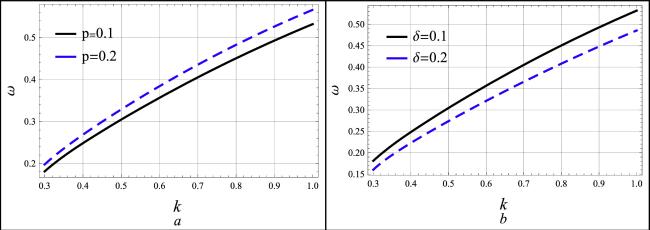
Figure 1. Variation of frequency ω(k) in two different scenarios: (a) with respect to the normalized ratio of positron density to electron density p, and (b) with respect to the ratio of positron density to ion density δ. The parameters used in the analysis are p = 0.1, θ = 2°, η = 0.1 and lz = 0.3. |
4. Small-amplitude nonlinear structure
To arrive at the damped KdV equation, we use a reductive perturbation approach. The independent spatial and temporal variables are transformed into stretched variables as follows:14 –20 ) and collecting the lowest order of ε, we obtain the relationship between different variables as follows, and the lowest order i.e. $\sim {\epsilon }^{\tfrac{3}{2}}$ of the ion continuity equation gives:23 )–(27 ), we obtain the following expression for the phase velocity of the IAW in the presence of Coriolis force when the magnetic field is quantized in dense degenerate plasma
$\begin{eqnarray*}\begin{array}{l}\xi ={\epsilon }^{1/2}({l}_{x}x+{l}_{z}z-\lambda t),\\ \tau ={\epsilon }^{3/2}t,\ \mathrm{and}\ \nu ={\epsilon }^{\tfrac{3}{2}}{v}_{0},\end{array}\end{eqnarray*}$
where the direction cosines along the x- and z-axes are lx and lz, respectively, such that ${l}_{x}^{2}+{l}_{z}^{2}=1.$ Here, λ represents the linearized phase velocity of the IAWs, and ε is a small parameter (0 < ε < 1) that quantifies the smallness of the perturbed amplitude relative to the equilibrium quantity. The perturbed variables are expanded in terms of the small expansion parameter ε as follows: $\begin{eqnarray}\left[\begin{array}{c}{n}_{i,e,p}\\ {v}_{{ix}}\\ {v}_{{iy}}\\ {v}_{{iz}}\\ {\rm{\Phi }}\end{array}\right]=\left[\begin{array}{c}1\\ 0\\ 0\\ 0\\ 0\end{array}\right]+\epsilon \left[\begin{array}{c}{n}_{i,e,p1}\\ \epsilon {v}_{{ix}1}\\ {\epsilon }^{\tfrac{1}{2}}{v}_{{iy}1}\\ {v}_{{iz}1}\\ {{\rm{\Phi }}}_{1}\end{array}\right]+{\epsilon }^{2}\left[\begin{array}{c}{n}_{i,e,p2}\\ \epsilon {v}_{{ix}2}\\ {\epsilon }^{\tfrac{1}{2}}{v}_{{iy}2}\\ {v}_{{iz}2}\\ {{\rm{\Phi }}}_{2}\end{array}\right]+....\end{eqnarray}$
By applying the above perturbation scheme in equations ( $\begin{eqnarray}{v}_{{iz}1}=\displaystyle \frac{\lambda }{{l}_{z}}{n}_{i1}.\end{eqnarray}$
In the presence of the Coriolis force, the lowest order of different components of the ion momentum equation gives the following set of equations: $\begin{eqnarray}{v}_{{iy}1}=\displaystyle \frac{{l}_{x}}{G}\displaystyle \frac{\partial {{\rm{\Phi }}}_{1}}{\partial \xi },\end{eqnarray}$
where $G={\omega }_{{ci}}+2{\rm{\Omega }}\cos \theta $ is the effective rotation frequency that is a combined representation of Larmor gyration of the particles and the mechanical rotation of the plasma $\begin{eqnarray}{v}_{{ix}1}=\displaystyle \frac{\lambda }{G}\displaystyle \frac{\partial {v}_{{iy}1}}{\partial \xi },\end{eqnarray}$
$\begin{eqnarray}{v}_{{iz}1}=\left(\displaystyle \frac{{l}_{z}}{\lambda }+\displaystyle \frac{2{\rm{\Omega }}\sin \theta {l}_{x}}{\lambda G}\right){{\rm{\Phi }}}_{1}.\end{eqnarray}$
Similarly, the lowest order ∼ε of Poisson's equation is written as; $\begin{eqnarray}{\alpha }_{e1}\left(1+\delta \right){{\rm{\Phi }}}_{1}-{n}_{i1}+\delta {\alpha }_{p1}{{\rm{\Phi }}}_{1}=0.\end{eqnarray}$
Using equations ( $\begin{eqnarray}{\lambda }^{2}=\left({l}_{z}^{2}+\displaystyle \frac{2{l}_{z}{l}_{x}{\rm{\Omega }}\sin \theta }{G}\right)\displaystyle \frac{1}{\left(\left(1+\delta \right){\alpha }_{e1}-\delta {\alpha }_{p1}\right)}.\end{eqnarray}$
We obtain the the dynamical equations in the next higher order of ε as follows.Collecting the next higher order, i.e. ∼ε5/2 from the continuity equation of ions gives the following equation;29 –32 ) as follows;34 ) is unable to provide a detailed description of numerous nonlinear waves seen in laboratory experiments [29] when the dispersion coefficient (B) has small or zero values. Therefore, it is essential to examine the impact of higher order, leading to the following damped KE
$\begin{eqnarray}\begin{array}{l}\lambda \displaystyle \frac{\partial {n}_{i2}}{\partial \chi }-{l}_{z}\displaystyle \frac{\partial {v}_{{iz}2}}{\partial \chi }\\ =\displaystyle \frac{\partial {n}_{i1}}{\partial \tau }+{l}_{x}\displaystyle \frac{\partial {v}_{{ix}1}}{\partial \chi }+{l}_{z}\displaystyle \frac{\partial \left({n}_{i1}{v}_{{iz}1}\right)}{\partial \chi }.\end{array}\end{eqnarray}$
The ∼ε5/2 of the x component of the momentum equation gives the following equation, $\begin{eqnarray}{l}_{x}\displaystyle \frac{\partial {{\rm{\Phi }}}^{(2)}}{\partial \chi }-{{Gv}}_{{iy}}^{(2)}=\lambda \displaystyle \frac{\partial {v}_{{ix}}^{(1)}}{\partial \chi }.\end{eqnarray}$
The ∼ε5/2 of the z component of the momentum equation of ions becomes $\begin{eqnarray}\begin{array}{l}\lambda \displaystyle \frac{\partial {v}_{{iz}}^{(2)}}{\partial \xi }-{l}_{z}\displaystyle \frac{\partial {{\rm{\Phi }}}^{(2)}}{\partial \xi }-2{\rm{\Omega }}\sin \theta {v}_{{iy}2}\\ =\displaystyle \frac{\partial {v}_{{iz}}^{(1)}}{\partial \tau }+{l}_{z}{v}_{{iz}}^{(1)}\displaystyle \frac{\partial {v}_{{iz}}^{(1)}}{\partial \xi }+{v}_{0}{v}_{{iz}}^{(1)}.\end{array}\end{eqnarray}$
The ∼ε2 of Poisson's equation gives the following equation; $\begin{eqnarray}\begin{array}{l}\left(1+\delta \right){\alpha }_{e1}{{\rm{\Phi }}}_{2}+\delta {\alpha }_{p1}{{\rm{\Phi }}}_{2}-{n}_{i2}\\ =\displaystyle \frac{{\partial }^{2}{{\rm{\Phi }}}_{1}}{\partial {\chi }^{2}}-\left(1+\delta \right){\alpha }_{e2}{\left({{\rm{\Phi }}}_{1}\right)}^{2}-\delta {\alpha }_{p2}{\left({{\rm{\Phi }}}_{1}\right)}^{2}.\end{array}\end{eqnarray}$
The damped KdV equation is obtained by solving equations ( $\begin{eqnarray}\begin{array}{l}\displaystyle \frac{\partial {{\rm{\Phi }}}_{1}}{\partial \tau }+A{{\rm{\Phi }}}_{1}\displaystyle \frac{\partial {{\rm{\Phi }}}_{1}}{\partial \xi }\\ +B\displaystyle \frac{{\partial }^{3}{{\rm{\Phi }}}_{1}}{\partial {\xi }^{3}}+D{{\rm{\Phi }}}_{1}=0,\end{array}\end{eqnarray}$
where the nonlinear A, and dispersive B and dissipative D coefficients obtained are given by; $\begin{eqnarray*}A=\displaystyle \frac{\tfrac{3}{{\lambda }^{2}}{\left({l}_{z}^{2}+\tfrac{2{l}_{z}{l}_{x}{\rm{\Omega }}\sin \theta }{G}\right)}^{2}-2{\lambda }^{2}\left(\left(1+\delta \right){\alpha }_{e2}+\delta {\alpha }_{p2}\right)}{\tfrac{2}{\lambda }\left({l}_{z}^{2}+\tfrac{2{l}_{z}{l}_{x}{\rm{\Omega }}\sin \theta }{G}\right)},\end{eqnarray*}$
$\begin{eqnarray*}B=\displaystyle \frac{{\lambda }^{2}\left(1+\tfrac{1}{G}\right)-\tfrac{{\lambda }^{2}}{{G}^{2}}\left({l}_{z}^{2}+\tfrac{2{l}_{z}{l}_{x}{\rm{\Omega }}\sin \theta }{G}\right)}{\tfrac{2}{\lambda }\left({l}_{z}^{2}+\tfrac{2{l}_{z}{l}_{x}{\rm{\Omega }}\sin \theta }{G}\right)},\end{eqnarray*}$
$\begin{eqnarray*}D=\displaystyle \frac{{v}_{0}}{2}.\end{eqnarray*}$
Equation ( $\begin{eqnarray}\begin{array}{l}{\partial }_{\tau }\varphi +A\varphi {\partial }_{\xi }\varphi +B{\partial }_{\xi }^{3}\varphi \\ -C{\partial }_{\xi }^{5}\varphi +D\varphi =0.\end{array}\end{eqnarray}$
Here, φ ≡ Φ1.5. Semi-analytic solution of the damped KE
To overcome the non-integrability of the damped KE, equation (35 ), we employ certain assumptions to derive a semi-analytic solution. In this analysis, we introduce the following ansatz:36 ) into the damped KE, equation (35), we can get37 ) under the assumptions ${Q}_{1}\left({\tau }_{0}\right)=1$ and ${\partial }_{\tau }{Q}_{3}\left({\tau }_{0}\right)=0$:37 ), we obtain the approximate analytical solution to equation (36 ):
$\begin{eqnarray}\varphi ={Q}_{1}\left(\tau \right)\tilde{{\rm{\Psi }}}(\xi {Q}_{2}\left(\tau \right),{Q}_{3}\left(\tau \right)).\end{eqnarray}$
The symbol $\tilde{{\rm{\Psi }}}(\xi {Q}_{2}\left(\tau \right),{Q}_{3}\left(\tau \right))$ represents an arbitrary perfect answer. Here, ${Q}_{1}\left(\tau \right)$, ${Q}_{2}^{-1}\left(\tau \right)$ and ${Q}_{3}\left(\tau \right)$ are the amplitude, width and velocity multiplied by the time of wave propagation, respectively. These parameters are critical in determining the properties of non-stationary waves, such as solitary waves and CWs. Inserting the ansatz in equation ( $\begin{eqnarray}\begin{array}{l}\left[{{AQ}}_{1}\left(\tau \right){Q}_{2}\left(\tau \right)\left({Q}_{1}\left(\tau \right)-{Q}_{2}{\left(\tau \right)}^{4}\right){\rm{\Psi }}+\xi {Q}_{1}\left(\tau \right){\partial }_{\tau }{Q}_{2}\left(\tau \right)\right]{\partial }_{\xi }\tilde{{\rm{\Psi }}}\\ +{{BQ}}_{1}\left(\tau \right)\left({Q}_{2}{\left(\tau \right)}^{3}-{Q}_{2}{\left(\tau \right)}^{5}\right){\partial }_{\xi }^{3}\tilde{{\rm{\Psi }}}+\left({{DQ}}_{1}\left(\tau \right)+{\partial }_{\tau }{Q}_{1}\left(\tau \right)\right)\tilde{{\rm{\Psi }}}\\ +{Q}_{1}\left(\tau \right)\left({\partial }_{\tau }{Q}_{3}\left(\tau \right)-{Q}_{2}{\left(\tau \right)}^{5}\right){\partial }_{\tau }\tilde{{\rm{\Psi }}}=0.\end{array}\end{eqnarray}$
We get, by solving the system in equation ( $\begin{eqnarray}\begin{array}{l}{Q}_{1}\left(\tau \right)={Q}_{2}{\left(\tau \right)}^{4},\\ {Q}_{2}\left(\tau \right)={{\rm{e}}}^{-\tfrac{1}{4}D\tilde{\tau }},\\ \mathrm{and}\\ {Q}_{3}\left(\tau \right)=\tfrac{4}{5D}(1-{{\rm{e}}}^{-\tfrac{5}{4}D\tilde{\tau }}),\end{array}\end{eqnarray}$
with $\tilde{\tau }=\left(\tau -{\tau }_{0}\right),$ where τ0 denotes the initial value of the propagation time. Substituting the values of Q1, Q2 and Q3 into equation ( $\begin{eqnarray}\varphi ={{\rm{e}}}^{-{DT}}\tilde{{\rm{\Psi }}}\left(\xi {{\rm{e}}}^{-\tfrac{1}{4}R\tilde{\tau }},\displaystyle \frac{4}{5D}\left(1-{{\rm{e}}}^{-\tfrac{5}{4}D\tilde{\tau }}\right)\right).\end{eqnarray}$
This is a general solution to the damped KE, equation (35), as well as to the study of dissipative solitary waves, CWs and other phenomena. The specific form of the dissipative solitary wave solution to the damped KE can be found in [31]: $\begin{eqnarray}\begin{array}{l}\varphi =\displaystyle \frac{105{B}^{2}}{169{AC}}{{\rm{e}}}^{-D\tilde{\tau }}\\ {{\rm{sech}} }^{4}\left[\displaystyle \frac{1}{\sqrt{52C/B}}\left(\xi {{\rm{e}}}^{-\tfrac{1}{4}D\tilde{\tau }}-\displaystyle \frac{36{B}^{2}}{169C}\displaystyle \frac{4}{5D}\left(1-{{\rm{e}}}^{-\tfrac{5}{4}D\tilde{\tau }}\right)\right)\right].\end{array}\end{eqnarray}$
Furthermore, the undamped (D = 0) KE, equation (35), confirms the analytical CW solution, as described in [31] $\begin{eqnarray}{\rm{\Psi }}=\displaystyle \frac{5{B}^{2}}{3\times 7\times {13}^{2}{AC}}{\left\{7+\sqrt{7\times 31}{{cn}}^{4}\left[\sqrt[4]{\displaystyle \frac{31}{7}}\sqrt{\displaystyle \frac{G}{78C}}\left(x-\displaystyle \frac{{2}^{7}{G}^{2}}{3\times {13}^{2}C}t\right);\displaystyle \frac{1}{\sqrt{2}}\right]\right\}}^{2}.\end{eqnarray}$
We obtain the damping CW solution of the damped KE, equation (35), by inserting the analytical CW solution, equation (41), into the general solution of the dissipative nonlinear structures, equation (39): $\begin{eqnarray}\varphi =\displaystyle \frac{5{B}^{2}{{\rm{e}}}^{-{DT}}}{3\times 7\times {13}^{2}{AC}}{\left\{7+\sqrt{7\times 31}{{cn}}^{4}\left[\sqrt[4]{\displaystyle \frac{31}{7}}\sqrt{\displaystyle \frac{B}{78C}}\left(\xi {{\rm{e}}}^{-\tfrac{1}{4}{DT}}-\displaystyle \frac{{2}^{9}{B}^{2}}{15\times {13}^{2}{CD}}\left(1-{{\rm{e}}}^{-\tfrac{5}{4}{DT}}\right)\right);\displaystyle \frac{1}{\sqrt{2}}\right]\right\}}^{2}.\end{eqnarray}$
6. Parametric analysis
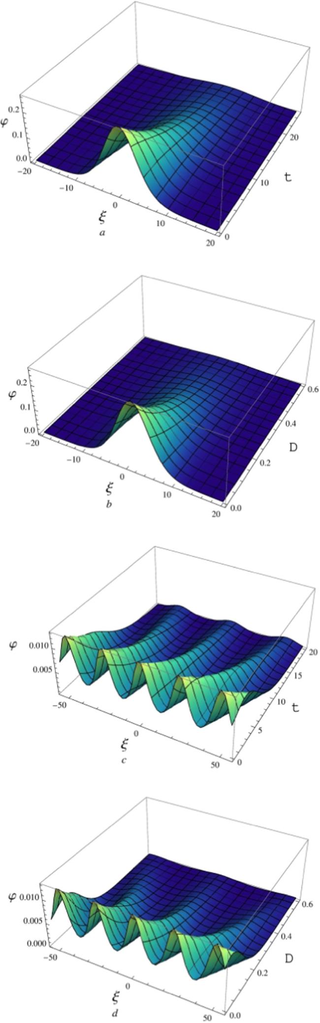
We examine the IAW excitations in e-p-i dense, homogeneous, magnetized and collisional plasmas in this section. Our parameters (in cgs units) are those of astrophysical plasma scenarios with mass 1.67 × 10⁻²⁴ g and charge 4.803 × 10⁻¹⁰ stat coulomb of hydrogen ions in a degenerate plasma system [32]. These situations are within the range n0 = 1026 − 1029cm−3, B0 = 106 − 109G and T = 107K. The parametric dependence of damped Kawahara solitons and damped Kawahara centroid waves on pertinent plasma properties will be covered in this section. The behavior of the damped Kawahara solitary solution φ of equation (40 ) is shown in figure (2) as a function of ξ for various values of the plasma, including the Landau quantization η, direction cosine (via lz), the normalized ratio of positron density to electron density p and the normalized ratio of positron density to ion density δ. It is clear that an increase in the ratio of the positron density to ion density δ, the direction cosine (via lz) and the Landau quantization η causes the waves to become broader and shorter. Specifically, a rise in δ, lz and η causes the structures' nonlinearity to diminish, which in turn causes the pulse amplitude to shrink, while an increase in δ, lz and η causes the dispersion to grow, which increases the pulse width. Conversely, as figure (2) illustrates, a rise in the normalized positron-to-electron density ratio p results in an increase in the damped Kawahara solitons' amplitude and a small alteration in the width. The pulse profiles of the IA damped Kawahara CWs φ of equation (42 ) vary for different levels of the angle of rotation θ, the magnetic field (via Ω), the direction cosine (via lz) and the normalized ratio of the positron density to electron density p, as shown in figure 3. It has been observed that higher values of p result in larger-amplitude ion acoustic CW profiles. Conversely, higher values of θ, lz and Ω lead to larger-amplitude ion acoustic CW profiles compared to lower values. In figure 4, the relationship between the amplitude of the damped Kawahara soliton and CWs and the coefficient of the damping term D and the propagation time t is depicted. It is evident from the figures that as D and t increase, both the amplitude of the soliton and the CW decrease. This trend suggests that the damping term and the propagation time have a damping effect on the waves, leading to their decrease in amplitude. This phenomenon is consistent with the properties of damped waves, wherein the energy of the wave is gradually dissipated over time. Therefore, an increase in D and t results in a weaker wave with a reduced amplitude.
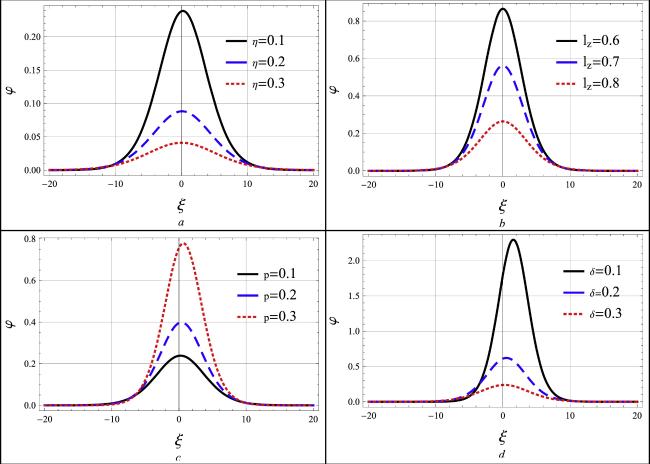
Figure 2. The profile of the damped Kawahara solitons solutions, equation (40), is depicted against ξ for different values of: (a) the Landau quantization η withT = 0.2, p = 0.1, δ = 0.3 and lz = 0.6; (b) the obliqueness angle lz withT = 0.2, p = 0.1, θ = 2°, η = 0.1 and δ = 0.3; (c) the normalized ratio of positron density to electron density p with δ = 0.3, θ = 2, η = 0.1 and lz = 0.6; (d) the ratio of positron density to ion density δ withT = 0.2, p = 0.1, θ = 2, η = 0.1 and lz = 0.6. |

Figure 3. The profile of the damped Kawahara CW solutions, equation (42), is depicted against ξ for different values of: (a) the angle of rotation θ, T = 0.2, δ = 0.2, Ω0 = 0.3, η = 0.1 and lz = 0.6; (b) the normalized ratio of positron density to electron density p with θ = 2°, δ = 0.2, Ω0 = 0.3, T = 0.2 and η = 0.1; (c) the obliqueness angle lz with θ = 2°, δ = 0.2, Ω0 = 0.3, T = 0.2 and η = 0.1; (d) the rotational frequency Ω0 with θ = 2°, δ = 0.2, η = 0.1, T = 0.2 and lz = 0.6. |
Figure 4. The profile of the damped Kawahara solitons and CW solutions is plotted with respect to the damping term D and the propagation time t. The parameters used in the plots are T = 0.2, p = 0.1, θ = 2°, Ω0 = 0.3, η = 0.1, δ = 0.3 and lz = 0.6. |
7. Summary
In this study, we have synthesized the key properties of IA damped Kawahara solitary waves and CWs in a dense, homogeneous, magnetized and collisional e-p-i plasma by employing Landau quantization of the magnetic field and considering the Coriolis force. The linear dispersion relation is obtained through the application of Fourier analysis, revealing that the frequency rises with higher p, while an increase in δ results in a decrease in frequency. The damped KdV equation was established by the application of the reductive perturbation technique. Nevertheless, at extremely low or zero values of the dispersion coefficient B, this equation does not provide an accurate description of waves in our system. As a result, we have examined the largest possible perturbation, which has resulted in the damped KE (also known as the damped fKdV equation). In this system, IA waves with only positive potentials form. As the ratio of positron density to electron density and the normalized temperature (as well as the angle of rotation θ, the ratio of positron density to ion density δ and the Landau quantization η) increase, the amplitude of IA CWs decreases (increases). The examination of the characteristics of IA damped Kawahara solitary waves and CWs in dense plasma settings in astrophysical contexts, especially in white dwarfs, may benefit from this work.