


1. Introduction
| • | It remains unclear whether the system permits a solution with mixed simple pole and high-order pole, even though it has been shown that the system has several special single-pole solutions [30, 31]. |
| • | Previously, the RH problem of the AB equation was solved using residue conditions instead of the Laurent expansion. |
| • | When the spectral parameters are pure imaginary, we obtain dark W-type soliton solutions, dark W-type double-pole solutions, and mixed dark W-type and double-pole solutions. The W-type solitons have been studied using modulation instability and Darboux transformation [33–35]. However, the latter two types of solitons are new and have not been reported in other literature. |
| • | The RH approach has not been used to study multiple high-order pole solutions for the AB system. |
2. The Riemann–Hilbert problem
2.1. Spectral analysis
${\omega }_{\pm }(x,t,\lambda )$ possess the following analytic properties:
| • | ${\omega }_{+,2}$, ${\omega }_{-,1}$ and s11 are continuous for ${C}^{+}\cup {\mathbb{R}}$ and can be analytically extended to ${C}^{+}$, |
| • | ${\omega }_{-,2}$, ${\omega }_{+,1}$ and s22 are continuous for ${C}^{-}\cup {\mathbb{R}}$ and can be analytically extended to ${C}^{-}$, |
2.2. Symmetries
2.3. Riemann–Hilbert problem
A multiplicative matrix RH problem is proposed:
| • | Analyticity : $P(x,t,\lambda )$ is analytic in ${\mathbb{C}}/{\mathbb{R}}$, |
| • | Jump condition: ${P}^{-}(x,t,\lambda )={P}^{+}(x,t,\lambda )J(x,t,\lambda )$, $\lambda \in {\mathbb{R}}$, |
| • | Asymptotic behaviors : $P(x,t,\lambda )\sim {\mathbb{I}}+O(\tfrac{1}{\lambda }),\quad \lambda \to \infty $, |
3. RH problem with high-order poles
3.1. RH problem with single high-order pole
With the rapidly decaying initial condition (
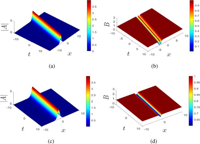
Figure 1. The single solution with parameters (1) ϱ1 = 1, λ0 = i. (2) ϱ1 = 1, λ0 = 2 + i. |
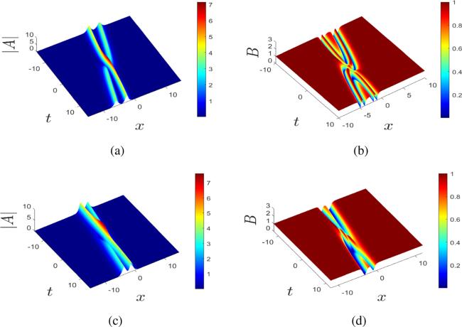
Figure 2. The second-order pole solution with parameters ϱ1 = 1, ϱ2 = 2. (1) λ0 = i. (2) λ0 = 1 + i. |
3.2. RH problem with multiple high-order poles
With the rapidly decaying initial condition (
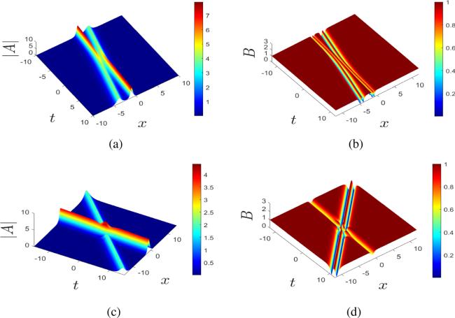
Figure 3. The two-soliton solution with parameters ϱ1,1 = ϱ2,1 = 1. (1) λ1 = i, λ2 = 2i. (2) λ1 = 2 + i, λ2 = 0.5i. |

Figure 4. A simple and a second-order pole solution with parameters ϱ1,1 = ϱ1,2 = ϱ2,1 = 1. (1) λ1 = 0.5i, λ2 = 2i. (2) λ1 = 0.5i, λ2 = 0.2 + 0.2i. (3) λ1 = 0.5 + 0.5i, λ2 = 0.2 + 0.2i. |