


1. Introduction
The eikonal approximation (EA) for quantum scattering was developed by Glauber [1]. As one of the most widely used approximations of quantum scattering problems, the EA was applied in numerous high-energy scattering problems of various physical systems, such as nuclear collisions [2–6], nuclear reactions [7–9], or the collisions between other types of high-energy particles [10–17]. The Hamiltonians of these scattering problems are given by the relevant natural interactions, and thus are time-independent.
On the other hand, in recent years the technique of manipulation of scattering processes with laser or other kinds of periodical external fields has been developed for various physical systems [18–30]. In the presence of the periodical field, the Hamiltonian of the scattering problem becomes a time-dependent one. These problems should be treated by the Floquet scattering theory [31–34], and the ‘original form' of the EA, which is developed for the scattering with time-independent Hamiltonian, cannot be directly applied.
In this work we generalize the EA to the scattering problems with periodical Hamiltonians. We derive the expressions of the scattering wave function and scattering amplitude given by the EA, and verify our results via the example of shaking spherical square-well potential.
Notice that the original EA was initially developed for the one-body potential scattering problem, and was later applied in more complicated scattering problems, e.g. the nuclear reaction problems [2–9]. Similarly, although in this work we focus on the one-body potential scattering, which is for simplicity, the generalized EA we developed can also be applied for more complicated scattering problems with periodical Hamiltonian.
The remainder of this paper is organized as follows. In section 2 we derive the generalized EA for the calculations of the Floquet scattering wave function, scattering amplitude and and cross section. In section 3 we apply the generalized EA for a periodical spherical square-well model, and show the applicability of our approach. There is a summary in section 4 . Some details of our calculation approach are shown in the appendix.
2. Generalized EA
In this section we generalize the EA for the Floquet scattering. We first derive the EA for the calculation of Floquet scattering wave function, and then calculate the Floquet scattering amplitude and cross section with the wave function obtained by the EA.
2.1. Scattering wave function
We consider the scattering of a single particle on a periodical potential, with the Hamiltonian being given by
$\begin{eqnarray}\begin{array}{l}\hat{H}=-\displaystyle \frac{{{\hslash }}^{2}}{2m}{{\rm{\nabla }}}^{2}+U({\boldsymbol{r}},t).\end{array}\end{eqnarray}$
Here m and r ≡ xex + yey + zez are the mass and position of the particle, respectively, with ex,y,z being the unit vector along the x, y, z directions. In addition, U(r, t) is the scattering potential, which is a periodical function of time and satisfies $\begin{eqnarray}\begin{array}{l}U({\boldsymbol{r}},t)=U\left({\boldsymbol{r}},t+T\right),\end{array}\end{eqnarray}$
with T being the period, and ${\mathrm{lim}}_{r\to \infty }U({\boldsymbol{r}},t)=0$.We consider the scattering process with incident momentum ℏk. Without loss of generality, in this work we assume k is along the z-direction, i.e.,
$\begin{eqnarray}\begin{array}{l}{\boldsymbol{k}}=k{{\boldsymbol{e}}}_{z}.\end{array}\end{eqnarray}$
According to the Floquet scattering theory, the corresponding scattering wave function $\Psi$(r, t) of our system satisfies the time-dependent Schrödinger equation $\begin{eqnarray}\begin{array}{l}{\rm{i}}{\hslash }\displaystyle \frac{\partial }{\partial t}{\rm{\Psi }}({\boldsymbol{r}},t)=\hat{H}{\rm{\Psi }}({\boldsymbol{r}},t),\end{array}\end{eqnarray}$
and can be written as $\begin{eqnarray}\begin{array}{l}{\rm{\Psi }}({\boldsymbol{r}},t)={{\rm{e}}}^{-{\rm{i}}{Et}/{\hslash }}\psi ({\boldsymbol{r}},t).\end{array}\end{eqnarray}$
Here ψ(r, t) is a periodic function satisfying $\begin{eqnarray}\begin{array}{l}\psi ({\boldsymbol{r}},t)=\psi ({\boldsymbol{r}},t+T),\end{array}\end{eqnarray}$
and E ≡ ℏ2k2/(2m) is the scattering energy, with k = ∣k∣.Now the question is how to derive the periodic function ψ(r, t). As in the derivations for the EA for time-independent potential [35], here we consider the high-energy cases with7 ), the scattering effect is weak, so that the wave function ψ(r, t) can be approximated as the product of the incident wave and a factor which is slowly varying in the spatial space, i.e.,6 ), φEA(r, t) is a a periodic function of t i.e.,5 ), (8 ) into the Schrodinger equation (4 ), we obtain the explicit equation satisfied by φEA(r, t):10 ) the term $(\tfrac{{{\hslash }}^{2}}{2m}){{\rm{\nabla }}}^{2}{\phi }_{\mathrm{EA}}({\boldsymbol{r}},t)$ is much less than $(\tfrac{{{\hslash }}^{2}}{2m})k\tfrac{\partial {\phi }_{\mathrm{EA}}({\boldsymbol{r}},t)}{\partial z}$, and thus can be ignored.3(3 The ignoring of the second derivative of a slowly-varying function is also used in the derivation of the traditional EA for time-independent potential [1, 35], as well as some other approximations, e.g. the slowly-varying profile approximation of quantum optics [36], the Wentzel–Kramers–Brillouin (WKB) approximation [35] and the EA of classical optics [37].) Then we obtain
$\begin{eqnarray}\begin{array}{l}k\gg 2\pi /{l}_{U},\ \ \ E\gg {U}_{* },\end{array}\end{eqnarray}$
where lU and U* are the characteristic length scale and characteristic strength of the potential U(r, t), respectively. Under the condition ( $\begin{eqnarray}\begin{array}{l}\psi ({\boldsymbol{r}},t)\approx \displaystyle \frac{1}{{\left(2\pi \right)}^{3/2}}{{\rm{e}}}^{{\rm{i}}{kz}}{\phi }_{\mathrm{EA}}({\boldsymbol{r}},t),\end{array}\end{eqnarray}$
where φEA(r, t) is a slowly-varying function of r In addition, due to the condition ( $\begin{eqnarray}\begin{array}{l}{\phi }_{\mathrm{EA}}({\boldsymbol{r}},t)={\phi }_{\mathrm{EA}}({\boldsymbol{r}},t+T).\end{array}\end{eqnarray}$
Furthermore, substituting equations ( $\begin{eqnarray}\begin{array}{l}\left[{\rm{i}}{\hslash }\displaystyle \frac{\partial }{\partial t}+\displaystyle \frac{{\rm{i}}{{\hslash }}^{2}k}{2m}\displaystyle \frac{\partial }{\partial z}+\displaystyle \frac{{{\hslash }}^{2}}{2m}{{\rm{\nabla }}}^{2}-U({\boldsymbol{r}},t)\right]{\phi }_{\mathrm{EA}}({\boldsymbol{r}},t)=0.\end{array}\end{eqnarray}$
Notice that φEA(r, t) is a slowly-varying function of r. Explicitly, the characteristic length scale l* of the spatial variation of φEA(r, t) satisfies 1/l* ≫ k. On the other hand, ∂φEA(r, t)/∂z and ∇2φEA(r, t) are on the order of φEA(r, t)/l* and ${\phi }_{\mathrm{EA}}({\boldsymbol{r}},t)/{l}_{* }^{2}$, respectively. As a result, in equation ( $\begin{eqnarray}\begin{array}{l}\left[{\rm{i}}\displaystyle \frac{\partial }{\partial t}+{\rm{i}}{v}_{z}\displaystyle \frac{\partial }{\partial z}-\displaystyle \frac{1}{{\hslash }}U({\boldsymbol{r}},t)\right]{\phi }_{\mathrm{EA}}({\boldsymbol{r}},t)=0,\end{array}\end{eqnarray}$
where vz = ℏk/m is the velocity of the incident particle.For the convenience of the following discussion, we define the vector b as the projection of the position r on the x–y plane, i.e.,11 ) can be expressed as14 )–(15 ) into equation (11 ). Additionally, φEA(r, t) tends to 1 in the limit z → −∞ for arbitrary t, as the slowly-varying wave function in the EA for time-independent potential, and satisfies the periodical condition (9 ). The latter fact can be directly proved via the fact $U({\boldsymbol{r}},t)=U\left({\boldsymbol{r}},t+T\right)$. Moreover, when U is independent of t, equation (14 ) becomes ${\phi }_{\mathrm{EA}}=\exp \{-{\rm{i}}\tfrac{1}{{v}_{z}{\hslash }}{\int }_{-\infty }^{z}U[{\boldsymbol{b}},z^{\prime} ]{\rm{d}}z^{\prime} \}$. This is just the slowly-varying part of the scattering wave function for time-independent potential, which is given by the traditional EA [35].
$\begin{eqnarray}\begin{array}{l}{\boldsymbol{b}}=x{{\boldsymbol{e}}}_{x}+y{{\boldsymbol{e}}}_{y}.\end{array}\end{eqnarray}$
Thus, the potential U(r, t) is also function of {b, z, t}, i.e., $\begin{eqnarray}\begin{array}{l}U({\boldsymbol{r}},t)=U({\boldsymbol{b}},z,t).\end{array}\end{eqnarray}$
We find that with the above notations, the solution of equation ( $\begin{eqnarray}\begin{array}{l}{\phi }_{\mathrm{EA}}({\boldsymbol{r}},t)=\exp \,\left\{-{\rm{i}}\displaystyle \frac{1}{{v}_{z}{\hslash }}{\displaystyle \int }_{-\infty }^{z}U\left[{\boldsymbol{b}},z^{\prime} ,\tilde{t}(t,z,z^{\prime} )\right]{\rm{d}}z^{\prime} \right\},\end{array}\end{eqnarray}$
where $\begin{eqnarray}\begin{array}{l}\tilde{t}(t,z,z^{\prime} )=t+\displaystyle \frac{z^{\prime} -z}{{v}_{z}}.\end{array}\end{eqnarray}$
One can verify this solution by directly substituting equations (In summary, the scattering wave function given by the generalized EA for the Floquet scattering is ${\rm{\Psi }}({\boldsymbol{r}},t)\,={\left(2\pi \right)}^{-3/2}{{\rm{e}}}^{-{\rm{i}}{Et}/{\hslash }}{{\rm{e}}}^{{\rm{i}}{kz}}{\phi }_{\mathrm{EA}}({\boldsymbol{r}},t)$, with the function φEA(r, t) being given by equation (14 ).4(4 Notice that the scattering wave function $\Psi$(r, t) given by EA is different from the one given by the semi-classical approximation (SCA) [38], which is the three-dimensional generalization of the Wentzel–Kramers–Brillouin (WKB) approximation. This difference can be explained as follows. For simplicity, we consider the case with a time-independent potential, and denote the scattering wave function given by the SCA as $\Psi$SCA(r). As shown in [38], the phase of $\Psi$SCA(r) is determined by the action of a classical trajectory with respect to r. Thus, for each r, to determine the value of $\Psi$SCA(r), one should solve an individual classical Hamiltonian equation, and then integrating the corresponding Lagrangian with time. In contrast, as shown in our main text, under the EA, one can derive the phase of the wave function (i.e., ${\rm{i}}\tfrac{1}{{v}_{z}{\rm{\hslash }}}{\int }_{-\infty }^{z}U[{\boldsymbol{b}},z^{\prime} ]{\rm{d}}z$ for the case with time-independent potential) by directly integrating the potential energy, without solving any classical dynamical equation. Additionally, we should also notice that the conditions of the WKB approximation and EA are different. Explicitly, the condition for the former can be expressed as k ≫ 2π/lU with our notations, while the one for EA is equation (7 ), i.e., both k ≫ 2π/lU and E ≫ U*.)
2.2. Scattering amplitude
Now we calculate the scattering amplitude via the Floquet scattering wave function $\Psi$(r, t) obtained above via the generalized EA.
For our scattering problem, since the potential U is time-dependent, the energy conservation is broken. As a result, for given incident momentum k, the kinetic energy of the particle after the scattering process can beA ), the scattering amplitude with respect to incident momentum k = ℏkez and outgoing momentum ${\boldsymbol{k}}^{\prime} $, which satisfyA )5 ). Substituting equation (8 ) into equation (19 ), we find that under the generalized EA, the Floquet scattering amplitude can be expressed as14 ).
$\begin{eqnarray}\begin{array}{l}{E}_{n}\equiv \displaystyle \frac{{{\hslash }}^{2}{k}^{2}}{2m}+n{\hslash }\omega ,\ \ \mathrm{with}\ n={n}_{* },{n}_{* }+1,\ldots ,\end{array}\end{eqnarray}$
where $\begin{eqnarray}\begin{array}{l}\omega =2\pi /T,\end{array}\end{eqnarray}$
and n* ≤ 0 is the minimum integer which satisfies E + nℏω ≥ 0. Furthermore, according to the Floquet scattering theory (appendix $\begin{eqnarray}\begin{array}{l}\displaystyle \frac{{{\hslash }}^{2}| {\boldsymbol{k}}^{\prime} {| }^{2}}{2m}={E}_{n},\ \ (n={n}_{* },{n}_{* }+1,\ldots ),\end{array}\end{eqnarray}$
is given by (appendix $\begin{eqnarray}\begin{array}{l}\quad f({\boldsymbol{k}}^{\prime} ,n\leftarrow {\boldsymbol{k}})\\ =\,-\displaystyle \frac{m\omega }{{\left(2\pi \right)}^{1/2}}{\displaystyle \int }_{0}^{2\pi /\omega }{\rm{d}}t{\displaystyle \int }_{-\infty }^{+\infty }{\rm{d}}{\boldsymbol{r}}{{\rm{e}}}^{-{\rm{i}}{\boldsymbol{k}}^{\prime} \cdot {\boldsymbol{r}}}{{\rm{e}}}^{{\rm{i}}n\omega t/{\hslash }}U({\boldsymbol{r}},t)\psi ({\boldsymbol{r}},t),\end{array}\end{eqnarray}$
where ψ(r, t) is related to the scattering wave function $\Psi$(r, t) via equation ( $\begin{eqnarray}\begin{array}{l}\quad f({\boldsymbol{k}}^{\prime} ,n\leftarrow {\boldsymbol{k}})\\ \approx \,-\displaystyle \frac{m\omega }{{\left(2\pi \right)}^{2}}{\displaystyle \int }_{0}^{T}{\rm{d}}t{\displaystyle \int }_{-\infty }^{+\infty }{\rm{d}}{\boldsymbol{r}}{{\rm{e}}}^{-{\rm{i}}({\boldsymbol{k}}^{\prime} -{\boldsymbol{k}})\cdot {\boldsymbol{r}}}{{\rm{e}}}^{{\rm{i}}n\omega t}U({\boldsymbol{r}},t){\phi }_{\mathrm{EA}}({\boldsymbol{r}},t),\end{array}\end{eqnarray}$
with the wave function φEA(r, t) being given by equation (Moreover, under the high-energy condition (7 ) of the EA, these scattering amplitudes with the outgoing momentum ${\hslash }{\boldsymbol{k}}^{\prime} $ satisfying21 ). As proven in appendix B , under the condition (21 ), the scattering amplitude $f({\boldsymbol{k}}^{\prime} ,0\leftarrow {\boldsymbol{k}})$ given by the EA (i.e., equation (20 )) can be further reduced to22 ) can be further approximated as (appendix B ):
$\begin{eqnarray}\begin{array}{l}| {\boldsymbol{k}}^{\prime} | =k\ \ \mathrm{and}\ \ | {\boldsymbol{k}}^{\prime} -{\boldsymbol{k}}| \ll k,\end{array}\end{eqnarray}$
(i.e., n = 0 and the angle between the incident and outgoing momentum is small) are much larger than the ones for the outgoing momentums not satisfying equation ( $\begin{eqnarray}\begin{array}{rcl} & & f({\boldsymbol{k}}^{\prime} ,0\leftarrow {\boldsymbol{k}})\\ & \approx & \displaystyle \frac{\omega {{\hslash }}^{2}k}{{\left(2\pi \right)}^{2}{\rm{i}}}{\displaystyle \int }_{0}^{T}\,{\rm{d}}t{\displaystyle \int }_{-\infty }^{+\infty }{\rm{d}}{\boldsymbol{b}}{{\rm{e}}}^{-{\rm{i}}({\boldsymbol{k}}^{\prime} -{\boldsymbol{k}})\,\cdot \,{\boldsymbol{b}}}\\ & & \times \left\{\exp \,\left(-{\rm{i}}\displaystyle \frac{1}{{v}_{z}{\hslash }}{\displaystyle \int }_{-\infty }^{+\infty }U\left[{\boldsymbol{b}},z^{\prime} ,\tilde{t}(t,z,z^{\prime} )\right]{\rm{d}}z^{\prime} \right)-1\right\}\\ & & (\mathrm{for}\ k=k^{\prime} ,\ \mathrm{and}\ \ | {\boldsymbol{k}}^{\prime} -{\boldsymbol{k}}| \ll k).\end{array}\end{eqnarray}$
Moreover, when the potential U(r, t) ≡ U(b, z, t) is independent of the direction of b, i.e., U(b, z, t) ≡ U(b, z, t), equation ( $\begin{eqnarray}\begin{array}{rcl} & & f({\boldsymbol{k}}^{\prime} ,0\leftarrow {\boldsymbol{k}})\\ & \approx \, & \displaystyle \frac{\omega {{\hslash }}^{2}k}{2\pi {\rm{i}}}{\displaystyle \int }_{0}^{T}\,{\rm{d}}t{\displaystyle \int }_{0}^{+\infty }b\,{\rm{d}}{{bJ}}_{0}({kb}\theta )\\ & & \times \left\{\exp \,\left(-{\rm{i}}\displaystyle \frac{1}{{v}_{z}{\hslash }}{\displaystyle \int }_{-\infty }^{+\infty }U\left[b,z^{\prime} ,\tilde{t}(t,z,z^{\prime} ),\right]{\rm{d}}z^{\prime} \right)-1\right\},\end{array}\end{eqnarray}$
where θ is the angle between k and ${{\boldsymbol{k}}}^{{\prime} }$, and J0 is the 0th order Bessel function of the first kind.2.3. Crosssection
Using the scattering amplitude $f({\boldsymbol{k}}^{\prime} ,n\leftarrow {\boldsymbol{k}})$ given by equation (20 ), one can further derive various cross section of the scattering process. In particular, the differential cross section with respect to outgoing kinetic energy En and outgoing momentum direction $\hat{{\boldsymbol{s}}}$ is
$\begin{eqnarray}\begin{array}{l}\displaystyle \frac{{\rm{d}}\sigma ({E}_{n},\hat{{\boldsymbol{s}}})}{{\rm{d}}\hat{{\boldsymbol{s}}}}=\sqrt{\displaystyle \frac{{k}_{n}}{k}}{\left|f({k}_{n}\hat{{\boldsymbol{s}}},n\leftarrow {\boldsymbol{k}})\right|}^{2},\end{array}\end{eqnarray}$
with ${k}_{n}=\sqrt{2{{mE}}_{n}/{\hslash }}$. Furthermore, according to the optical theorem, the total cross section with respect to incident momentum k is $\begin{eqnarray}{\sigma }_{\mathrm{tot}}(k)=\displaystyle \frac{4\pi }{k}\mathrm{Im}\left[f({\boldsymbol{k}},0\leftarrow {\boldsymbol{k}})\right].\end{eqnarray}$
3. Results for shaking spherical square-well model
Now we illustrate the generalized EA derived above via an example. Explicitly, we consider the scattering of a particle on a spherical square-well with shaking depth (figure 1(a)):
$\begin{eqnarray}\begin{array}{l}U({\boldsymbol{r}},t)=\left\{\begin{array}{cc}{U}_{0}\cos (\omega t)+{U}_{1}, & r\leqslant {r}_{0}\\ 0, & r\gt {r}_{0}\end{array}\right.,\end{array}\end{eqnarray}$
with r0 being the width of the square well, ω being the shaking angular frequency, and U0(1) being the amplitude of the shaking (non-shaking) parts of the well depth. In the following discussions we use the natural unit ℏ = m = r0 = 1.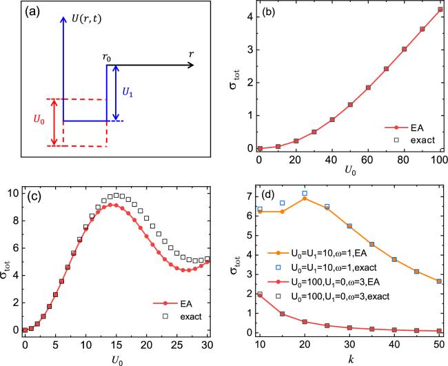
Figure 1. (a) Schematic diagram of the spherical square-well with shaking depth. (b)–(d) Total scattering cross section σtot(k) of the shaking square-well model. Here we show the results given by the exact numerical calculations (squares) and the generalized EA (dots connected by solid lines) we developed in this work. In these figures all the parameters are given with natural unit ℏ = 2m = r0 = 1. (b): σtot(k) as a function of U0, for the systems with U1 = 0, k = 37, and ω = 10. (c) σtot(k) as a function of U0, for the case with U1 = 10U0, k = 37, ω = 1. (d) σtot(k) as a function of k, for the case with U0 = U1 = 10 and ω = 1 (orange dots connected by lines, and blue squares) and U0 = 100,U1 = 0 and ω = 3 (red dots connected by lines, and black squares). |
We calculate the total cross section σtot(k) for various parameters, with both the exact numerical approach and the generalized EA developed in the above sections (equations (25 ) and (23 )). In figures 1(b) and (c) we show the σtot as functions of the shaking amplitude U0 for the cases with fixed U1, ω and k. Additionally, in figure 1(d) we show the σtot as a function of incident momentum k, for the cases with fixed U0,1 and ω.
Figures 1(b)–(d) show that for these parameters the results given by the generalized EA consist very well of the ones given by exact numerical calculation. These results show the applicability of the generalized EA.
Moreover, the error of the generalized EA is slightly increased when U0 ≳ 15, for the system of figure 1(c) with U1 = 10U0. This may be explained as follows. For this system when U0 ≳ 15 the depth U1 of the static part of the square well is as large as 150. As a result, the condition E ≫ U* of equation (7 ) is not satisfied as well as in the cases with small U0. Similarly, for the system of figure 1(d) the error of the generalized EA is slightly increased in the cases with small incident momentum k because in these cases the high-energy condition (7 ) is not satisfied so well.
4. Summary
In this work we generalize the EA for the Floquet scattering problems with periodical potential. We further demonstrate the generalized EA with the example of a shaking spherical square-well model. The approach we developed can be used in the theoretical studies for the external-field manipulation of collisions between particles, e.g. the laser manipulation of collisions between atoms, nucleons or electrons.
Appendix A. Floquet scattering amplitude
In this appendix we show why Floquet scattering amplitude can be expressed as in equation (19 ). For a Floquet scattering problem with Hamiltonian $\hat{H}$ of equation (1 ), the explicit scattering state $\Psi$(r, t) with respect to incident momentum k satisfies the Schrödinger equation (4 ), and can be expressed as $\Psi$(r, t) = e−iEt/ℏψ(r, t), with E = ℏ2k2/(2m) and ψ(r, t) = ψ(r, t + T), as shown in section II. Furthermore, the wave function ψ(r, t) also satisfies the long-range outgoing boundary conditionA1 ), i.e.,
$\begin{eqnarray}\begin{array}{l}\mathop{\mathrm{lim}}\limits_{r\to \infty }\psi ({\boldsymbol{r}},t)=\displaystyle \frac{1}{{\left(2\pi \right)}^{3/2}}\left[{{\rm{e}}}^{{\rm{i}}{\boldsymbol{k}}\cdot {\boldsymbol{r}}}+\displaystyle \sum _{n={n}_{* }}^{+\infty }\displaystyle \frac{{f}_{n}(\hat{{\boldsymbol{r}}})}{r}{{\rm{e}}}^{{\rm{i}}{k}_{n}r}{{\rm{e}}}^{-{\rm{i}}n\omega t}\right],\end{array}\end{eqnarray}$
where $\hat{{\boldsymbol{r}}}\equiv {\boldsymbol{r}}/r$ is the direction vector of r, and ${k}_{n}=\sqrt{2m(E+n{\hslash }\omega )/{\hslash }}$. Furthermore, the Floquet scattering amplitude with respect to the incident momentum k and outgoing momentum ${k}_{n}\hat{{\boldsymbol{r}}}$ is defined as the factor ${f}_{n}(\hat{{\boldsymbol{r}}})$ in equation ( $\begin{eqnarray}f({\boldsymbol{k}}^{\prime} ,n\leftarrow {\boldsymbol{k}})\equiv {f}_{n}(\hat{{\boldsymbol{k}}}^{\prime} )\ \mathrm{of}\ \mathrm{Eq}.({\rm{A}}1).\end{eqnarray}$
Now our task is to prove the scattering amplitude defined in equation (A2 ) can be expressed as in equation (19 ). For convenience, here we formally introduce the Hilbert space ${{\mathscr{H}}}_{F}$, which is defined as the set of all periodical functions η(t) which satisfies η(t) = η(t + T). We denote the vector of ${{\mathscr{H}}}_{F}$ as ∣), and define the basis of ${{\mathscr{H}}}_{F}$ as:
$\begin{eqnarray}\begin{array}{l}| s)\equiv {{\rm{e}}}^{-{\rm{i}}s\omega t},\ \ \ \ \ (s=0,\pm 1,\pm 2,\,\ldots ).\end{array}\end{eqnarray}$
We further the inner product of two periodical functions η(t) and $\eta ^{\prime} (t)$ as $\begin{eqnarray}\begin{array}{l}(\eta ^{\prime} | \eta )=\displaystyle \frac{1}{T}{\displaystyle \int }_{0}^{T}\eta ^{\prime} {\left(t\right)}^{* }\eta (t){\rm{d}}t,\end{array}\end{eqnarray}$
which yields that Span{∣0), ∣ ± 1), ∣ ± 2), …} is a group of orthogonal basis of ${{\mathscr{H}}}_{F}$.Now we consider the wave function ψ(r, t) of our problem. Due to the periodical condition ψ(r, t) = ψ(r, t + T), ψ(r, t) is a r-dependent element of ${{\mathscr{H}}}_{F}$, and can be denoted as ∣ψ[r]). Explicitly, we have the notation correspondence:A1 ) of ψ(r, t) can be re-expressed as
$\begin{eqnarray}\begin{array}{l}\psi ({\boldsymbol{r}},t)=\displaystyle \sum _{s=-\infty }^{+\infty }{\psi }_{s}({\boldsymbol{r}}){{\rm{e}}}^{-{\rm{i}}s\omega t}\ \Longleftrightarrow | \psi [{\boldsymbol{r}}])=\displaystyle \sum _{s=-\infty }^{+\infty }{\psi }_{s}({\boldsymbol{r}})| s).\end{array}\end{eqnarray}$
Moreover, with the new notation the equation satisfied by ψ(r, t) can be re-expressed as $\begin{eqnarray}\begin{array}{l}\hat{{ \mathcal H }}| \psi [{\boldsymbol{r}}])=E| \psi [{\boldsymbol{r}}]),\end{array}\end{eqnarray}$
with $\begin{eqnarray}\begin{array}{l}\hat{{ \mathcal H }}=-\displaystyle \frac{{{\hslash }}^{2}}{2m}{{\rm{\nabla }}}^{2}\otimes \hat{{ \mathcal I }}+\displaystyle \sum _{s=-\infty }^{+\infty }{U}_{s}({\boldsymbol{r}}){\hat{{ \mathcal C }}}^{s}.\end{array}\end{eqnarray}$
Here $\hat{{ \mathcal I }}$ is the unit operator of ${{\mathscr{H}}}_{F}$, and $\hat{{ \mathcal C }}\,={\sum }_{n=-\infty }| n+1)(n| $. In addition, the functions Us(r) (s = 0, ± 1, ± 2, …) are related to the potential U(r, t) via $\begin{eqnarray}\begin{array}{l}U({\boldsymbol{r}},t)=\displaystyle \sum _{s=-\infty }^{+\infty }{U}_{s}({\boldsymbol{r}}){{\rm{e}}}^{-{\rm{i}}s\omega t}.\end{array}\end{eqnarray}$
Furthermore, the long-range boundary condition ( $\begin{eqnarray}\begin{array}{l}\mathop{\mathrm{lim}}\limits_{r\to \infty }| \psi [{\boldsymbol{r}}])=\displaystyle \frac{1}{{\left(2\pi \right)}^{3/2}}\left[{{\rm{e}}}^{{\rm{i}}{\boldsymbol{k}}\cdot {\boldsymbol{r}}}| 0)+\displaystyle \sum _{n={n}_{* }}^{+\infty }\displaystyle \frac{{f}_{n}(\hat{{\boldsymbol{r}}})}{r}{{\rm{e}}}^{{\rm{i}}{k}_{n}r}| n)\right].\end{array}\end{eqnarray}$
The above results yield that the term ${f}_{n}(\hat{{\boldsymbol{r}}})$, which is originally defined in equation (A1 ), is also the scattering amplitude of the latter scattering problem with Hamiltonian time-independent $\hat{{ \mathcal H }}$ and incident wave function $\tfrac{{{\rm{e}}}^{{\rm{i}}{\boldsymbol{k}}\cdot {\boldsymbol{r}}}}{{\left(2\pi \right)}^{3/2}}| 0)$. Notice that this scattering problem is defined in the product space ${\mathscr{H}}\otimes {{\mathscr{H}}}_{F}$. Since $\hat{{ \mathcal H }}$ is time-independent, we can use the standard scattering theory to analyze the properties of the scattering amplitude. Using equation (A2 ) and the scattering theory, we finally haveA3 )–(A9 ), we directly find that equation (A10 ) is just equation (19 ).
$\begin{eqnarray}\begin{array}{l}f({\boldsymbol{k}}^{\prime} ,n\leftarrow {\boldsymbol{k}})\equiv {f}_{n}(\hat{{\boldsymbol{k}}}^{\prime} )=-{\left(2\pi \right)}^{1/2}m\\ \times \displaystyle \int {\rm{d}}{\boldsymbol{r}}{{\rm{e}}}^{-{\rm{i}}{k}_{n}\hat{{\boldsymbol{k}}}^{\prime} \cdot {\boldsymbol{r}}}\left(n| \left[\displaystyle \sum _{s=-\infty }^{+\infty }{U}_{s}({\boldsymbol{r}}){\hat{{ \mathcal C }}}^{s}\right]| \psi [{\boldsymbol{r}}]\right).\end{array}\end{eqnarray}$
Using equations (Appendix B. Derivations of equations (22 ) and (23 )
In this appendix we derive equations (22 ) and (23 ) of the main text. We first notice that, under the condition (21 ), ${\boldsymbol{k}}^{\prime} -{\boldsymbol{k}}$ is approximately perpendicular to the direction of k (i.e., the z-direction), and thus $({\boldsymbol{k}}^{\prime} -{\boldsymbol{k}})\cdot {\boldsymbol{r}}\approx ({\boldsymbol{k}}^{\prime} -{\boldsymbol{k}})\cdot {\boldsymbol{b}}$. Substituting this result and the conditions n = 0 into equation (20 ), we obtain11 ) yields thatB2 ) into equation (B1 ), and using the property (9 ) of φEA(r, t), as well as the facts14 ) of φEA(r, t) and mvz = ℏk, we immediately obtain equation (22 ).
$\begin{eqnarray}\begin{array}{l}f({\boldsymbol{k}}^{\prime} ,0\leftarrow {\boldsymbol{k}})\approx -\displaystyle \frac{m\omega }{{\left(2\pi \right)}^{2}}{\displaystyle \int }_{0}^{T}{\rm{d}}t{\displaystyle \int }_{-\infty }^{+\infty }{\rm{d}}{\boldsymbol{b}}\\ \times {\displaystyle \int }_{-\infty }^{+\infty }{\rm{d}}z\left\{{{\rm{e}}}^{-{\rm{i}}({\boldsymbol{k}}^{\prime} -{\boldsymbol{k}})\cdot {\boldsymbol{b}}}U({\boldsymbol{r}},t){\phi }_{\mathrm{EA}}({\boldsymbol{r}},t)\right\}.\end{array}\end{eqnarray}$
Furthermore, equation ( $\begin{eqnarray}\begin{array}{l}U({\boldsymbol{r}},t){\phi }_{\mathrm{EA}}({\boldsymbol{r}},t)={\rm{i}}{\hslash }\displaystyle \frac{\partial }{\partial t}{\phi }_{\mathrm{EA}}({\boldsymbol{r}},t)+{\rm{i}}{\hslash }{v}_{z}\displaystyle \frac{\partial }{\partial z}{\phi }_{\mathrm{EA}}({\boldsymbol{r}},t).\end{array}\end{eqnarray}$
Substituting equation ( $\begin{eqnarray}{\left.{\phi }_{\mathrm{EA}}({\boldsymbol{r}},t)\right|}_{z=-\infty }=1;\end{eqnarray}$
$\begin{eqnarray}\begin{array}{l}{\left.{\phi }_{\mathrm{EA}}({\boldsymbol{r}},t)\right|}_{z=+\infty }\\ \,=\exp \,\left\{-{\rm{i}}\displaystyle \frac{1}{{v}_{z}{\hslash }}\right.\\ \,\left.{\int }_{-\infty }^{+\infty },\times U\left[{\boldsymbol{b}},z^{\prime} ,\tilde{t}(t,z,z^{\prime} )\right]{\rm{d}}z^{\prime} \right\},\end{array}\end{eqnarray}$
which are given by the expression (Furthermore, when the potential U(b, z, t) = U(b, z, t) is independent of the direction of b. In this case $f({\boldsymbol{k}}^{\prime} -{\boldsymbol{k}})$ only depends on the norm $k=| {\boldsymbol{k}}| =| {\boldsymbol{k}}^{\prime} | $ and the angle θ between k and ${\boldsymbol{k}}^{\prime} $. Without loss of generality, we take the direction of ${\boldsymbol{k}}^{\prime} -{\boldsymbol{k}}$ to be along the x-axis, and define φ to be the angle between b and the x-axis. Since we consider the cases with small θ, we haveB5 ) into equation (22 ), and using the facts $\int {\boldsymbol{b}}={\int }_{0}^{+\infty }b{\rm{d}}b{\int }_{0}^{2\pi }{\rm{d}}\phi $, and ${\int }_{0}^{2\pi }{{\rm{e}}}^{-{\rm{i}}\alpha \cos \phi }\,{\rm{d}}\phi =2\pi {J}_{0}(\alpha )$, we can obtain equation (23 ).
$\begin{eqnarray}({\boldsymbol{k}}^{\prime} -{\boldsymbol{k}})\cdot {\boldsymbol{b}}\approx k\theta b\cos \phi .\end{eqnarray}$
Substituting equation (