


1. Introduction
Optical nonreciprocal transmission, which allows the propagation of photons in one direction while there is suppression in the opposite one, has been widely studied in various physical systems, such as atomic systems [1, 2], cavity quantum electrodynamic (cavity-QED) systems [3–5], waveguide-QED systems [6, 7], optomechanical or electromechanical systems [8–10] and parity-time-symmetry optical systems [11–13], due to its potential applications in quantum communication and quantum information processing [14, 15]. In particular, waveguide-QED [16–19], which enables strongly light–matter interaction at single-photon level and long-range interactions between remote emitters in a 1D waveguide, provides an ideal platform for the manipulation of nonreciprocal single-photon scattering. To date, with the development of quantum technology, waveguide-QED systems can be experimentally implemented in several setups, including superconducting qubits coupled to transmission lines [20–23], quantum dots coupled to photonic crystal waveguides [24–27] and ultracold atoms coupled to optical fibers [28–30]. Many waveguide-QED-based nonreciprocal quantum devices with high contrast ratio have been realized [31–38].
In the above-mentioned studies, the emitters are generally considered to be much smaller than the wavelength of the propagating photons in the 1D waveguide, wherein the emitter can be viewed as a point, and dipole approximation is usually adopted to describe the interactions between the emitter and the waveguide photons [39]. However, once the size of the emitter is comparable or even larger than the wavelength of the waveguide photons, the dipole approximation will be invalid and a so-called ‘giant atom' theory should be applied to deal with the atom-photon interaction instead [40]. In the giant atom setup, the atom can couple to the waveguide via multiple separate points, which has been realized in several systems, including superconducting qubits coupled to surface acoustic waves (or transmission lines) [41–43] and cold atoms coupled to optical lattices [44]. A series of tempting quantum phenomena induced by the phase-dependent interference between different coupling points have been observed, such as frequency-dependent Lamb shifts and relaxation rates [45], non-exponential decay [46, 47], decoherence-free interaction [48–50], unconditional bound states [51–55] and quantum Zeno and anti-Zeno effects [56]. Recently, single-photon scattering in a waveguide-QED system containing giant atoms has also been broadly investigated and various giant atom-based single-photon devices have been realized [57–61]. For instance, with the help of chiral couplings and local or nonlocal phase effects, high-efficiency single-photon diodes [62], circulators [63] and frequency converters [64] can be achieved by coupling the giant atoms to a 1D waveguide.
In this paper, we further investigate the nonreciprocal single-photon scattering mediated by a three-level giant atom with two driving fields. We focus on exploring how to effectively control the nonreciprocal single-photon scattering and realizing perfect nonreciprocal transmission by manipulating the extra driving fields, including the Rabi frequencies, driving phases and the driving detuning. Two cases, i.e. with or without the driving fields, are discussed in detail. The results show that, in the absent of the driven fields, the giant atom degenerates into a two-level system, where the nonreciprocal single-photon scattering can be realized by tuning the local coupling phases between the giant atom and the waveguide, and an ideal diode for resonant photons with perfect contrast ratio can be achieved. In the presence of the driven fields, which introduces more tunable parameters to manipulate the nonreciprocal single-photon scattering behavior, a perfect frequency-tunable diode for photons with arbitrary frequencies can be achieved by properly adjusting the Rabi frequencies and phase difference of the two extra driving fields. Furthermore, the driving detuning also plays an important role in manipulating the nonreciprocal single-photon scattering. Both the location and width of each optimal nonreciprocal transmission window can be effectively modulated by the driving detuning. These remarkable features should be meaningful for designing nonreciprocal single-photon devices with wide or narrow bandwidth and may also have potential applications in quantum information processing. For instance, single-photon diodes with narrow band can significantly enhance the system sensitivity, resolution, and processing efficiency, which are pivotal in applications requiring high-frequency selectivity and precise control, such as precise sensing and spectral analysis [65]. Wide-band diodes can markedly improve data transmission rates and provide more comprehensive spectral information, which play an important role in applications requiring a broad frequency response [66].
The rest of the paper is organized as follows. In section 2 , we introduce the theoretical model of the double-driving Λ-type giant atom waveguide-QED structure and derive the analytical expressions of the transmission probabilities of photons from two opposite sides using a full quantum mechanical method. In section 3 , we show how perfect nonreciprocal transmission can be achieved with or without the extra driving field. The influence of the local coupling phases between the giant atom and the waveguide, the accumulation phase between the two waveguide coupling points, the Rabi frequencies and phase difference of the two driven fields and the driving detuning on the nonreciprocal single-photon scattering are discussed in detail. Finally, a conclusion is drawn in section 4 .
2. Model and basic theory
The model under consideration is shown in figure 1. A Λ-type three-level giant atom couples to the 1D waveguide via the transition $\left|e\right\rangle \leftrightarrow \left|g\right\rangle $ at two separate points $x=0$ and $x={x}_{0}$ with coupling strengths ${V}_{j=1,2}={V}_{j}{{\rm{e}}}^{{\rm{i}}{\phi }_{j}},$ respectively. ${\phi }_{j=1,2}$ are the corresponding local coupling phases. The other transition $\left|e\right\rangle \leftrightarrow \left|s\right\rangle $ is decoupled from the waveguide but driven by two classical laser beams with detuning ${{\rm{\Delta }}}_{L}$ and Rabi frequencies ${{\rm{\Omega }}}_{1}$ and ${{\rm{\Omega }}}_{2}{{\rm{e}}}^{{\rm{i}}\alpha },$ where $\alpha $ denotes the phase difference between the two driven lasers.
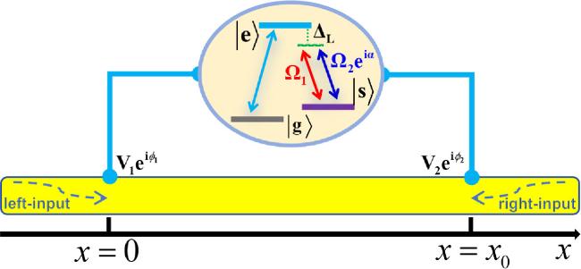
Figure 1. Schematic diagram of the giant waveguide-QED system. Giant atom contains a ground state $\left|g\right\rangle ,$ an excited state $\left|e\right\rangle $ and a metastable state $\left|s\right\rangle .$ Transition between states $\left|e\right\rangle $ and $\left|g\right\rangle $ is coupled by the waveguide mode at two separate points $x=0$ and $x={x}_{0}$ with coupling strengths ${V}_{j}{{\rm{e}}}^{{\rm{i}}{\phi }_{j}}$($j=1,2$) and ${\phi }_{j=1,2}$ are the corresponding coupling phases. Transition between states $\left|e\right\rangle $ and $\left|s\right\rangle $ is driven by two classical fields with detuning ${{\rm{\Delta }}}_{L}.$ ${{\rm{\Omega }}}_{1},$ ${{\rm{\Omega }}}_{2}$ and $\alpha $ are the corresponding Rabi frequencies and phase difference between the two driven lasers. |
The total Hamiltonian of the system described in figure 1 can be divided into three parts as,
$\begin{eqnarray}H={H}_{a}+{H}_{w}+{H}_{aw}.\end{eqnarray}$
The first term denotes the Hamiltonian of the giant atom. Under the rotating wave approximation, ${H}_{a}$ can be written as ($\hslash =1$),
$\begin{eqnarray}\begin{array}{l}{H}_{a}=\left({\omega }_{e}-{\rm{i}}\displaystyle \frac{{\gamma }_{e}}{2}\right){\sigma }_{ee}+\left({\omega }_{e}-{{\rm{\Delta }}}_{L}-{\rm{i}}\displaystyle \frac{{\gamma }_{s}}{2}\right){\sigma }_{ss}\\ \,\,+\,\left[\left({{\rm{\Omega }}}_{1}+{{\rm{\Omega }}}_{2}{{\rm{e}}}^{{\rm{i}}\alpha }\right){\sigma }_{es}+{\rm{H}}{\rm{.c}}.\right],\end{array}\end{eqnarray}$
where ${\omega }_{e}$ is the eigenfrequency of the state $\left|e\right\rangle .$ ${\sigma }_{m,n=e,s,g}$ is the dipole transition operator. ${\gamma }_{e}$ and ${\gamma }_{s}$ are the dissipations of the state $\left|e\right\rangle $ and $\left|s\right\rangle ,$ respectively. ${\rm{H}}{\rm{.c}}.$ represents the Hermitian conjugate.The second term in equation (1 ) represents the free Hamiltonian of the 1D waveguide, which can be expressed in the real space as,
$\begin{eqnarray}{H}_{w}=\displaystyle \int {\rm{d}}x{\hat{c}}_{R}^{\dagger }\left(x\right)\left(-{\rm{i}}{\upsilon }_{g}\displaystyle \frac{\partial }{\partial x}\right){\hat{c}}_{R}\left(x\right)+\displaystyle \int {\rm{d}}x{\hat{c}}_{L}^{\dagger }\left(x\right)\left({\rm{i}}{\upsilon }_{g}\displaystyle \frac{\partial }{\partial x}\right){\hat{c}}_{L}\left(x\right),\end{eqnarray}$
where ${\upsilon }_{g}$ is the group velocity of the waveguide photons. ${\hat{c}}_{R}^{\dagger }\left(x\right)$ [${\hat{c}}_{R}\left(x\right)$] and ${\hat{c}}_{L}^{\dagger }\left(x\right)$[${\hat{c}}_{L}\left(x\right)$] denote the bosonic creation (annihilation) operators for the right-moving and the left-moving photon at position $x$ in the waveguide.The third term in equation (1 ) describes the interaction Hamiltonian between the giant atom and the waveguide photons, which can be given by,
$\begin{eqnarray}\begin{array}{l}{H}_{aw}={V}_{1}{{\rm{e}}}^{{\rm{i}}{\phi }_{1}}\displaystyle \displaystyle \sum _{S=L,R}\displaystyle \int {\rm{d}}x\delta \left(x\right){\hat{c}}_{S}^{\dagger }\left(x\right){\sigma }_{ge}\\ \,+\,{V}_{2}{{\rm{e}}}^{{\rm{i}}{\phi }_{2}}\displaystyle \displaystyle \sum _{S=L,R}\displaystyle \int {\rm{d}}x\delta \left(x-{x}_{0}\right){\hat{c}}_{S}^{\dagger }\left(x\right){\sigma }_{ge}+{\rm{H}}{\rm{.c}}\mathrm{.}\end{array}\end{eqnarray}$
Since the excitation number in the system is conserved under the rotating wave approximation, in the single-excitation subspace, the eigenstate of $H$ can be written as,
$\begin{eqnarray}\begin{array}{l}\left|{\rm{\Psi }}\right\rangle =\displaystyle \int {\rm{d}}x{\phi }_{R}\left(x\right){\hat{c}}_{R}^{\dagger }\left(x\right)\left|0,g\right\rangle +\displaystyle \int {\rm{d}}x{\phi }_{L}\left(x\right){\hat{c}}_{L}^{\dagger }\left(x\right)\left|0,g\right\rangle \\ \,+\,{u}_{e}\left|0,e\right\rangle +{u}_{s}\left|0,s\right\rangle ,\end{array}\end{eqnarray}$
where ${\phi }_{R,L}(x)$ represent the probability amplitudes for producing the rightward and leftward moving photons at position $x$ in the waveguide, respectively. $\left|0,m\right\rangle \left(m=g,e,s\right)$ represents no photon in the system, and the giant atom is in the state $\left|m\right\rangle .$ ${u}_{e}$ and ${u}_{s}$ correspond to the probability amplitudes of state $\left|e\right\rangle $ and $\left|s\right\rangle ,$ respectively. By solving the stationary eigenequation $H\left|{\rm{\Psi }}\right\rangle =\omega \left|{\rm{\Psi }}\right\rangle ,$ we can obtain the following linear differential equations: $\begin{eqnarray*}\begin{array}{l}0=\left(-{\rm{i}}{\upsilon }_{{\rm{g}}}\displaystyle \frac{\partial }{\partial x}-\omega \right){\phi }_{R}\left(x\right)+{V}_{1}{{\rm{e}}}^{{\rm{i}}{\phi }_{1}}\delta \left(x\right){u}_{e}\\ \,+\,{V}_{2}{{\rm{e}}}^{{\rm{i}}{\phi }_{2}}\delta \left(x-{x}_{0}\right){u}_{e},\\ 0=\left({\rm{i}}{\upsilon }_{{\rm{g}}}\displaystyle \frac{\partial }{\partial x}-\omega \right){\phi }_{L}\left(x\right)+{V}_{1}{{\rm{e}}}^{{\rm{i}}{\phi }_{1}}\delta \left(x\right){u}_{e}\\ \,+\,{V}_{2}{{\rm{e}}}^{{\rm{i}}{\phi }_{2}}\delta \left(x-{x}_{0}\right){u}_{e},\end{array}\end{eqnarray*}$
$\begin{eqnarray}\begin{array}{l}0={V}_{1}{{\rm{e}}}^{-{\rm{i}}{\phi }_{1}}\left[{\phi }_{R}\left(0\right)+{\phi }_{L}\left(0\right)\right]+{V}_{2}{{\rm{e}}}^{-{\rm{i}}{\phi }_{2}}\left[{\phi }_{R}\left({x}_{0}\right)+{\phi }_{L}\left({x}_{0}\right)\right]\\ \,+\,\left({\omega }_{e}-{\rm{i}}\displaystyle \frac{{\gamma }_{e}}{2}-\omega \right){u}_{e}+\left({{\rm{\Omega }}}_{1}+{{\rm{\Omega }}}_{2}{{\rm{e}}}^{{\rm{i}}\alpha }\right){u}_{s},\\ 0=\left({\omega }_{e}-{{\rm{\Delta }}}_{L}-{\rm{i}}\displaystyle \frac{{\gamma }_{s}}{2}-\omega \right){u}_{s}+\left({{\rm{\Omega }}}_{1}+{{\rm{\Omega }}}_{2}{{\rm{e}}}^{-{\rm{i}}\alpha }\right){u}_{e}.\end{array}\end{eqnarray}$
We first consider a photon with wave vector $k$ incident from the left side of the waveguide, then the wave functions ${\phi }_{R}\left(x\right)$ and ${\phi }_{L}\left(x\right)$ can be expressed as,7 ) and (8 ) into equation (6 ), we obtain:
$\begin{eqnarray}{\phi }_{R}\left(x\right)={{\rm{e}}}^{{\rm{i}}kx}\left\{{\theta }\left(-x\right)+A\left[\theta \left(x\right)-\theta \left(x-{x}_{0}\right)\right]+t\theta \left(x-{x}_{0}\right)\right\},\end{eqnarray}$
$\begin{eqnarray}{\phi }_{L}\left(x\right)={{\rm{e}}}^{-{\rm{i}}kx}\left\{r\theta \left(-x\right)+B\left[\theta \left(x\right)-\theta \left(x-{x}_{0}\right)\right]\right\},\end{eqnarray}$
where $\theta \left(x\right)$ is the Heaviside step function with $\theta \left(0\right)=1/2.$ $t$ and $r$ respectively represent the transmission and reflection amplitudes in the region $x\gt {x}_{0}$ and $x\lt 0.$ $A$ and $B$ are defined as the probability amplitudes for the rightward and leftward moving photons between the two coupling points. Substituting equations ( $\begin{eqnarray}t=\displaystyle \frac{{\rm{i}}\left({\rm{\Delta }}-E\right)-2{\rm{i}}\sqrt{{{\rm{\Gamma }}}_{1}{{\rm{\Gamma }}}_{2}}\,\sin \,\theta {{\rm{e}}}^{{\rm{i}}\phi }-{\gamma }_{e}/2}{{\rm{i}}\left({\rm{\Delta }}-E\right)-{{\rm{\Gamma }}}_{1}-{{\rm{\Gamma }}}_{2}-2\sqrt{{{\rm{\Gamma }}}_{1}{{\rm{\Gamma }}}_{2}}{{\rm{e}}}^{{\rm{i}}\theta }\,\cos \,\phi -{\gamma }_{e}/2},\end{eqnarray}$
$\begin{eqnarray}r=\displaystyle \frac{{{\rm{\Gamma }}}_{1}+{{\rm{\Gamma }}}_{2}{{\rm{e}}}^{2{\rm{i}}\theta }+2\sqrt{{{\rm{\Gamma }}}_{1}{{\rm{\Gamma }}}_{2}}{{\rm{e}}}^{{\rm{i}}\theta }\,\cos \,\phi }{{\rm{i}}\left({\rm{\Delta }}-E\right)-{{\rm{\Gamma }}}_{1}-{{\rm{\Gamma }}}_{2}-2\sqrt{{{\rm{\Gamma }}}_{1}{{\rm{\Gamma }}}_{2}}{{\rm{e}}}^{{\rm{i}}\theta }\,\cos \,\phi -{\gamma }_{e}/2},\end{eqnarray}$
where ${\rm{\Delta }}=\omega -{\omega }_{e}$ is the frequency detuning between the incident photon and the atomic transition. $\theta =k{x}_{0}$ and $\phi ={\phi }_{2}-{\phi }_{1}$ are the accumulation phase and the coupling phase difference between the two local coupling points. ${{\rm{\Gamma }}}_{j=1,2}={V}_{j}^{2}/{\upsilon }_{g},$ and $E={{\rm{\Omega }}}^{2}/\left({\rm{\Delta }}+{{\rm{\Delta }}}_{L}\right)$ with ${\rm{\Omega }}\,=\sqrt{{{{\rm{\Omega }}}_{1}}^{2}+{{{\rm{\Omega }}}_{2}}^{2}+2{{\rm{\Omega }}}_{1}{{\rm{\Omega }}}_{2}\,\cos \,\alpha }$ the effective Rabi frequency of the two driven lasers. Here, we have assumed ${\gamma }_{s}=0.$When a single photon is incident from the right side of the waveguide, the wave functions ${\phi ^{\prime} }_{R}\left(x\right)$ and ${\phi ^{\prime} }_{L}\left(x\right)$ can be rewritten as,
$\begin{eqnarray}{\phi ^{\prime} }_{R}\left(x\right)=\left\{r^{\prime} \theta \left(x-{x}_{0}\right)+B^{\prime} \left[\theta \left(x\right)-\theta \left(x-{x}_{0}\right)\right]\right\}{{\rm{e}}}^{{\rm{i}}kx},\end{eqnarray}$
$\begin{eqnarray}\begin{array}{l}{\phi ^{\prime} }_{L}\left(x\right)=\left\{\theta \left(x-{x}_{0}\right)+A^{\prime} \left[\theta \left(x\right)-\theta \left(x-{x}_{0}\right)\right]\right.\\ \,\left.+\,t^{\prime} \theta \left(-x\right)\right\}{{\rm{e}}}^{-{\rm{i}}kx}.\end{array}\end{eqnarray}$
Similarly, by substituting equations (11 ) and (12 ) into equation (6 ), the transmission and reflection amplitudes can be obtained as,
$\begin{eqnarray}t^{\prime} =\displaystyle \frac{{\rm{i}}\left({\rm{\Delta }}-E\right)-2{\rm{i}}\sqrt{{{\rm{\Gamma }}}_{1}{{\rm{\Gamma }}}_{2}}\,\sin \,\theta {{\rm{e}}}^{-{\rm{i}}\phi }-{\gamma }_{e}/2}{{\rm{i}}\left({\rm{\Delta }}-E\right)-{{\rm{\Gamma }}}_{1}-{{\rm{\Gamma }}}_{2}-2\sqrt{{{\rm{\Gamma }}}_{1}{{\rm{\Gamma }}}_{2}}{{\rm{e}}}^{{\rm{i}}\theta }\,\cos \,\phi -{\gamma }_{e}/2},\end{eqnarray}$
$\begin{eqnarray}r^{\prime} =\displaystyle \frac{{{\rm{\Gamma }}}_{1}+{{\rm{\Gamma }}}_{2}{{\rm{e}}}^{-2{\rm{i}}\theta }+2\sqrt{{{\rm{\Gamma }}}_{1}{{\rm{\Gamma }}}_{2}}{{\rm{e}}}^{-{\rm{i}}\theta }\,\cos \,\phi }{{\rm{i}}\left({\rm{\Delta }}-E\right)-{{\rm{\Gamma }}}_{1}-{{\rm{\Gamma }}}_{2}-2\sqrt{{{\rm{\Gamma }}}_{1}{{\rm{\Gamma }}}_{2}}{{\rm{e}}}^{{\rm{i}}\theta }\,\cos \,\phi -{\gamma }_{e}/2}.\end{eqnarray}$
To quantitatively analyze the nonreciprocal single-photon scattering properties in the waveguide, we introduce the dimensionless quantities ${T}_{L}=| t{| }^{2}$ and ${T}_{R}=| t^{\prime} {| }^{2}$ for describing the transmission probabilities for photons incident from the left and right side, respectively.
3. Results and discussion
3.1. Nonreciprocal single-photon scattering with ${\rm{\Omega }}=0$
We first study the nonreciprocal single-photon scattering properties with ${\rm{\Omega }}=0.$ In this case, the three-level giant atom system degenerates into a two-level one. According to equations (9 ) and (13 ), we can obtain the two transmission coefficients ${T}_{L}$ and ${T}_{R}$ as,15 ) and (16 ) that the necessary condition to observe the optical nonreciprocity is $2{\rm{\Gamma }}\,\sin \,\theta \,\sin \,\phi -{\gamma }_{e}/2\,\ne 2{\rm{\Gamma }}\,\sin \,\theta \,\sin \,\phi +{\gamma }_{e}/2,$ which means that the nonreciprocity results from the combination effects of the atomic dissipation, the coupling phase difference and the accumulation phase between the two coupling points.
$\begin{eqnarray}\begin{array}{c}{T}_{L}\\ =\,\displaystyle \frac{{\left({\rm{\Delta }}-2{\rm{\Gamma }}\,\sin \,\theta \,\cos \,\phi \right)}^{2}+{\left(2{\rm{\Gamma }}\,\sin \,\theta \,\sin \,\phi -{\gamma }_{e}/2\right)}^{2}}{{\left({\rm{\Delta }}-2{\rm{\Gamma }}\,\sin \,\theta \,\cos \,\phi \right)}^{2}+{\left(2{\rm{\Gamma }}+2{\rm{\Gamma }}\,\cos \,\theta \,\cos \,\phi +{\gamma }_{e}/2\right)}^{2}},\end{array}\end{eqnarray}$
$\begin{eqnarray}\begin{array}{c}{T}_{R}\\ =\,\displaystyle \frac{{\left({\rm{\Delta }}-2{\rm{\Gamma }}\,\sin \,\theta \,\cos \,\phi \right)}^{2}+{\left(2{\rm{\Gamma }}\,\sin \,\theta \,\sin \,\phi +{\gamma }_{e}/2\right)}^{2}}{{\left({\rm{\Delta }}-2{\rm{\Gamma }}\,\sin \,\theta \,\cos \,\phi \right)}^{2}+{\left(2{\rm{\Gamma }}+2{\rm{\Gamma }}\,\cos \,\theta \,\cos \,\phi +{\gamma }_{e}/2\right)}^{2}},\end{array}\end{eqnarray}$
with ${{\rm{\Gamma }}}_{1}={{\rm{\Gamma }}}_{2}\equiv {\rm{\Gamma }}.$ It is well known that the nonreciprocal single-photon transmission requires ${T}_{L}\ne {T}_{R}.$ Thus, it is clear from equations (To quantitatively describe the optical nonreciprocity, the contrast ratio is introduced as $C=\tfrac{{T}_{R}-{T}_{L}}{{T}_{R}+{T}_{L}},$ which can be expressed as,
$\begin{eqnarray}C=\displaystyle \frac{2{\gamma }_{e}{\rm{\Gamma }}\,\sin \,\theta \,\sin \,\phi }{{\left({\rm{\Delta }}-2{\rm{\Gamma }}\,\sin \,\theta \,\cos \,\phi \right)}^{2}+{\left(2{\rm{\Gamma }}\,\sin \,\theta \,\sin \,\phi \right)}^{2}+{\left({\gamma }_{e}/2\right)}^{2}}.\end{eqnarray}$
From equation (17 ), one finds that the maximum of the contrast ratio can be obtained when ${\rm{\Delta }}=2{\rm{\Gamma }}\,\sin \,\theta \,\cos \,\phi ,$ which is given by,
$\begin{eqnarray}{C}_{{\rm{\max }}}=\displaystyle \frac{2{\gamma }_{e}{\rm{\Gamma }}\,\sin \,\theta \,\sin \,\phi }{{\left(2{\rm{\Gamma }}\,\sin \,\theta \,\sin \,\phi \right)}^{2}+{\left({\gamma }_{e}/2\right)}^{2}},\end{eqnarray}$
where ${C}_{\max }=\pm 1$ indicates the perfect nonreciprocal transmission.In this part, we focus on exploring the influence of the local coupling phases on the nonreciprocal scattering behavior. In figure 2, we plot the transmission coefficients ${T}_{L},$ ${T}_{R}$ and the contrast ratio $C$ as a function of the frequency detuning ${\rm{\Delta }}/{\rm{\Gamma }}$ for different phase differences $\phi ={\phi }_{2}-{\phi }_{1},$ i.e. $\phi =\left(\pi /4,\pi /2,3\pi /4\right),$ under the conditions $\theta =\pi /2$ and ${\gamma }_{e}=4{\rm{\Gamma }}.$ It is found that ${T}_{L}$ displays a Lorentzian line shape with phase-dependent Lamb shift. The location of the deep dip with height close to zero is determined by ${\rm{\Delta }}=2{\rm{\Gamma }}\,\sin \,\theta \,\cos \,\phi ,$ which is reduced to ${\rm{\Delta }}=2{\rm{\Gamma }}\,\cos \,\phi $ in the present case with $\theta =\pi /2.$ By increasing $\phi $ from 0 to $\pi ,$ the location of the dip shifts from ${\rm{\Delta }}=2{\rm{\Gamma }}$ to ${\rm{\Delta }}=-2{\rm{\Gamma }},$ as shown by the blue solid lines.
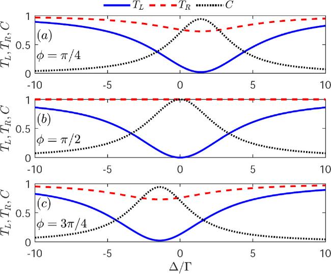
Figure 2. Transmission probabilities ${T}_{L},$ ${T}_{R}$ and the contrast ratio $C$ as a function of the frequency detuning ${\rm{\Delta }}/{\rm{\Gamma }}$ for different phase differences $\phi .$ Other common parameters are ${{\rm{\Omega }}}_{1}={{\rm{\Omega }}}_{2}=0,$ $\theta =\pi /2$ and ${\gamma }_{e}=4{\rm{\Gamma }}$. |
Furthermore, other than the location, the value of the dip is also strongly dependent on $\phi ,$ and the local coupling phase has a distinct influence on ${T}_{L}$ and ${T}_{R},$ which is the origin of the nonreciprocity. As can be seen, ${T}_{R}$ exhibits a similar line shape with a dip located at the same place as that of ${T}_{L},$ but the dip became much shallower when the height approached 1, as shown by the red dashed lines. Obviously, the transmission probability of photons incident from the right side is much larger than that from the left, which means that the incident photons with fixed frequency can nonreciprocally be transmitted with a high contrast ratio, as shown by the black dotted lines. A maximum $C=1$ can be obtained at the resonant point by tuning the phase difference to be $\phi =\pi /2,$ as shown in figure 2(b). In this case, the right-incident photons can be completely transmitted to the left with ${T}_{R}\equiv 1,$ while the left-incident resonant photons will be completely blocked with ${T}_{L}=0.$ Similar behavior, i.e. $C=-1$ with ${T}_{L}\equiv 1$ and ${T}_{R}=0,$ can be obtained by tuning the phase difference to be $\phi =3\pi /2$ within the region $\pi \lt \phi \lt 2\pi $ (as discussed below). These results imply that the local coupling phases can function as a sensitive controller to the single-photon nonreciprocal scattering.
To further demonstrate the phase-dependent nonreciprocal transmission in a more general case, the transmission coefficients ${T}_{L},$ ${T}_{R}$ and the contrast ratio $C$ as a function of the detuning ${\rm{\Delta }}/{\rm{\Gamma }}$ and phase difference $\phi $ are plotted in figure 3. It is shown in figure 3(a) that there is a wide red zone with ${T}_{L}\equiv 1$ around $\phi =3\pi /2,$ which means that the left-incident photons keep on propagating along the waveguide without absorption. This phenomenon can be understood through equation (15 ). It can be seen that ${T}_{L}\equiv 1$ over the whole range of the frequency detuning ${\rm{\Delta }}$ if $2{\rm{\Gamma }}\,\sin \,\theta \,\sin \,\phi \,-{\gamma }_{e}/2$ $=\pm \left(2{\rm{\Gamma }}+2{\rm{\Gamma }}\,\cos \,\theta \,\cos \,\phi +{\gamma }_{e}/2\right),$ which can be satisfied under the conditions $\theta =\pi /2,$ ${\gamma }_{e}=4{\rm{\Gamma }}$ and $\phi =3\pi /2.$ Physically, in the present case, if the phase difference is tuned to be $\phi =3\pi /2,$ the effective coupling strength between the giant atom and the waveguide $-2{\rm{\Gamma }}\left(1+\,\sin \,\theta \,\sin \,\phi \right)$ becomes zero, which means that the giant atom is decoupled from the waveguide. Thus, the left-incident photons can be freely transmitted. Furthermore, there is a bright blue zone corresponding to the transmission dip with ${T}_{L}\to 0.$ The location and value of the dip are phase sensitive, as discussed in figure 2, and a minimum ${T}_{L}=0$ can be obtained at the resonant point due to the perfect destructive interference between the direct photon path (i.e. along the waveguide) and the indirect one (i.e. be absorbed at $x=0,$ then re-emitted at $x={x}_{0}$ by the atom).

Figure 3. Contour map of the transmission probabilities ${T}_{L},$ ${T}_{R}$ and the contrast ratio $C$ as the function of both ${\rm{\Delta }}/{\rm{\Gamma }}$ and $\phi /\pi $ in (a), (b) and (c), respectively. Other common parameters are the same as those shown in figure 2. |
By comparing figures 3(a) and (b), one finds that the transmission probabilities ${T}_{L}$ and ${T}_{R}$ have opposite responses to the phase difference $\phi .$ For example, ${T}_{R}\equiv 1$ with $\phi =\pi /2,$ while ${T}_{L}\left({\rm{\Delta }}=0\right)=0.$ Figure 3(c) shows the contrast ratio of the transmission probabilities of the left-moving and right-moving photons. As expected, there is a phase shift optimal nonreciprocal transmission window denoted by the bright red or blue zones. The maximum $C=\pm 1$ is obtained by tuning the phase difference to be $\phi =\pi /2$ and $\phi =3\pi /2,$ respectively. Based on the analysis above, perfect single-photon nonreciprocal transmission for resonant photons can be realized by manipulating the local coupling phases and an ideal phase sensitive single-photon diode with perfect contrast ratio $C=\pm 1$ can be achieved.
3.2. Nonreciprocal single-photon scattering with ${\rm{\Omega }}\ne 0$
In this section, we focus on discussing how to control the nonreciprocal scattering characteristics of the single photons by manipulating the two driving fields. The transmission coefficients ${T}_{L}$ and ${T}_{R}$ that can be obtained through equations (9 ) and (13 ), read as follows:
$\begin{eqnarray}\begin{array}{c}{T}_{L}\\ =\,\displaystyle \frac{{\left({\rm{\Delta }}-E-2{\rm{\Gamma }}\,\sin \,\theta \,\cos \,\phi \right)}^{2}+{\left(2{\rm{\Gamma }}\,\sin \,\theta \,\sin \,\phi -{\gamma }_{e}/2\right)}^{2}}{{\left({\rm{\Delta }}-E-2{\rm{\Gamma }}\,\sin \,\theta \,\cos \,\phi \right)}^{2}+{\left(2{\rm{\Gamma }}+2{\rm{\Gamma }}\,\cos \,\theta \,\cos \,\phi +{\gamma }_{e}/2\right)}^{2}},\end{array}\end{eqnarray}$
$\begin{eqnarray}\begin{array}{l}{T}_{R}\\ =\,\displaystyle \frac{{\left({\rm{\Delta }}-E-2{\rm{\Gamma }}\,\sin \,\theta \,\cos \,\phi \right)}^{2}+{\left(2{\rm{\Gamma }}\,\sin \,\theta \,\sin \,\phi +{\gamma }_{e}/2\right)}^{2}}{{\left({\rm{\Delta }}-E-2{\rm{\Gamma }}\,\sin \,\theta \,\cos \,\phi \right)}^{2}+{\left(2{\rm{\Gamma }}+2{\rm{\Gamma }}\,\cos \,\theta \,\cos \,\phi +{\gamma }_{e}/2\right)}^{2}}.\end{array}\end{eqnarray}$
Accordingly, the contrast ratio can be expressed by,
$\begin{eqnarray}\begin{array}{c}C\\ =\,\displaystyle \frac{2{\gamma }_{e}{\rm{\Gamma }}\,\sin \,\theta \,\sin \,\phi }{{\left({\rm{\Delta }}-E-2{\rm{\Gamma }}\,\sin \,\theta \,\cos \,\phi \right)}^{2}+{\left(2{\rm{\Gamma }}\,\sin \,\theta \,\sin \,\phi \right)}^{2}+{\left({\gamma }_{e}/2\right)}^{2}}.\end{array}\end{eqnarray}$
Initially, we analyze how the local phase difference influences the nonreciprocal scattering characteristics under the conditions ${\rm{\Omega }}\equiv {{\rm{\Omega }}}_{1}=3{\rm{\Gamma }}$ and ${{\rm{\Omega }}}_{2}=0,$ where only one driving field with certain intensity is taken into account. Figure 4 shows the variations of ${T}_{L},$ ${T}_{R}$ and $C$ on the detuning ${\rm{\Delta }}/{\rm{\Gamma }}$ with different $\phi .$ As shown by the blue solid lines, ${T}_{L}$ displays a resonant transmission peak with ${T}_{L}=1$ and two phase shift sideband dips with ${T}_{L}\to 0$ located at ${\rm{\Delta }}={\rm{\Gamma }}\,\cos \,\phi \pm \sqrt{{{\rm{\Omega }}}^{2}+{{\rm{\Gamma }}}^{2}{\cos }^{2}\phi },$ which is significantly different from that in the case of ${\rm{\Omega }}=0.$ This is because, when the driving field is applied, the atomic transition $\left|e\right\rangle \leftrightarrow \left|s\right\rangle $ will lead to two dressed states with eigenfrequencies ${\omega }_{\pm }={\omega }_{e}+{\rm{\Gamma }}\,\cos \,\phi \pm \sqrt{{{\rm{\Omega }}}^{2}+{{\rm{\Gamma }}}^{2}{\cos }^{2}\phi },$ respectively. Thus, whenever the incident photons have frequency resonant with the two dressed states, nearly complete transmission blocking with ${T}_{L}=0$ occurs due to the destructive interference between the directly transmitted and re-emitted photons, as discussed above.
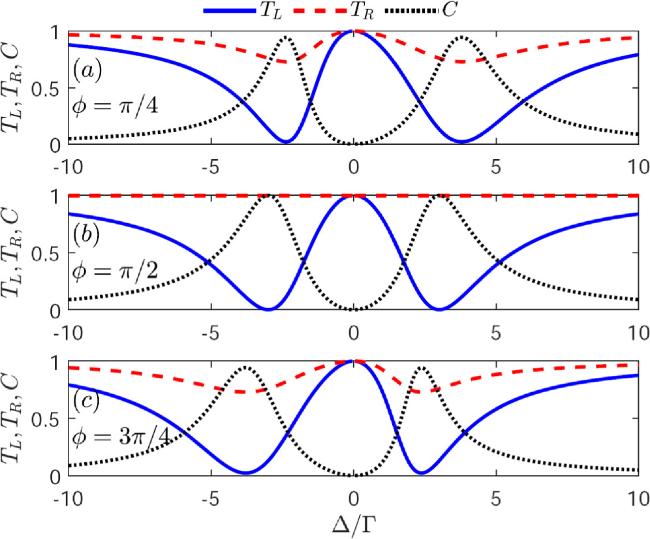
Figure 4. Transmission probabilities ${T}_{L},$ ${T}_{R}$ and the contrast ratio $C$ as a function of the frequency detuning ${\rm{\Delta }}/{\rm{\Gamma }}$ for different phase differences $\phi .$ Other common parameters are ${{\rm{\Omega }}}_{1}=3{\rm{\Gamma }},$ ${{\rm{\Omega }}}_{2}=0,$ $\theta =\pi /2$ and ${\gamma }_{e}=4{\rm{\Gamma }}$. |
Similar line shapes can be obtained for ${T}_{R}$ (see the red dashed lines), but with two shallower valleys, which results in a high contrast ratio, as denoted by the black dotted lines. The valleys can even disappear with ${T}_{R}\equiv 1$ when $\phi =\pi /2,$ and accordingly, a maximum $C=1$ can be obtained, as shown in figure 4(b). However, it is noteworthy that, unlike the two-level system with ${\rm{\Omega }}=0,$ here both the left-moving and right-moving resonant photons can freely transmit along the waveguide with $C\left({\rm{\Delta }}=0\right)=0,$ which means that the nonreciprocal transmission disappears. This can be explained from equations (19 ) and (20 ), wherein ${T}_{L}={T}_{R}\equiv 1$ when ${\rm{\Delta }}=0.$
In order to provide direct insight into the effect of the local coupling phases on the global behavior of the transmission probabilities and the contrast ratio, the contour map of ${T}_{L},$ ${T}_{R}$ and $C$ as the function of ${\rm{\Delta }}$ and $\phi $ are plotted in figure 5. It can be seen that there are two phase-dependent optimal nonreciprocal transmission windows located around ${\rm{\Delta }}={\rm{\Gamma }}\,\cos \,\phi \pm \sqrt{{{\rm{\Omega }}}^{2}+{{\rm{\Gamma }}}^{2}{\cos }^{2}\phi }.$ By tuning the local coupling phase difference $\phi ,$ both the position and width of the two windows can effectively be adjusted. A maximum contrast ratio $C=\pm 1$ can be obtained when $\phi $ is tuned to be $\phi =\pi /2$ or $\phi =3\pi /2.$ This implies that the perfect nonreciprocal transmission can be achieved for an incident photon with non-resonant frequencies, e.g. ${\rm{\Delta }}=\pm {\rm{\Omega }},$ which can be further modulated by manipulating the Rabi frequencies and the corresponding phase difference of the two driving fields, as discussed below.
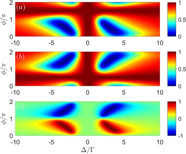
Figure 5. Contour map of the transmission probabilities ${T}_{L},$ ${T}_{R}$ and the contrast ratio $C$ as the function of both ${\rm{\Delta }}/{\rm{\Gamma }}$ and $\phi /\pi $ in (a), (b) and (c), respectively. Other common parameters are the same as those shown in figure 4. |
To investigate the influence of the Rabi frequency of the driving field on the nonreciprocal single-photon scattering, the contrast ratio $C$ as a function of the detuning ${\rm{\Delta }}/{\rm{\Gamma }}$ for different Rabi frequencies, and the corresponding contour map with respect to ${\rm{\Delta }}/{\rm{\Gamma }}$ and ${\rm{\Omega }}$ under the conditions $\phi =\theta =\pi /2,$ ${{\rm{\Omega }}}_{2}=0$ and ${\gamma }_{e}=4{\rm{\Gamma }}$ are plotted in figures 6(a) and (b), respectively. It is found that the spectra of $C$ display the vacuum Rabi splitting-like line shapes with two peaks located at ${\rm{\Delta }}={\rm{\Gamma }}\,\sin \,\theta \,\cos \,\phi \pm \sqrt{{{\rm{\Omega }}}^{2}+{{\rm{\Gamma }}}^{2}{\sin }^{2}\theta {\cos }^{2}\phi },$ as shown in figure 6(a). According to the locations of the two peaks, we can obtain the separation between them, which is determined by $D=2\sqrt{{{\rm{\Omega }}}^{2}+{{\rm{\Gamma }}}^{2}{\sin }^{2}\theta {\cos }^{2}\phi }$ (corresponding to $D=2{\rm{\Omega }}$ in the present case). As can be seen, the separation of the two peaks increases monotonically with the increase of ${\rm{\Omega }}.$ Namely, the larger the Rabi frequency, the wider the separation, which can be seen more clearly from the contour map of $C$ in figure 6(b). In principle, the separation can be enlarged over the entire frequency range, which means that perfect nonreciprocal transmission for a single photon with arbitrary frequency can be realized by properly tuning the Rabi frequency and choosing other system parameters. This also implies that a frequency-tunable single-photon diode with an ideal contrast ratio can be achieved.
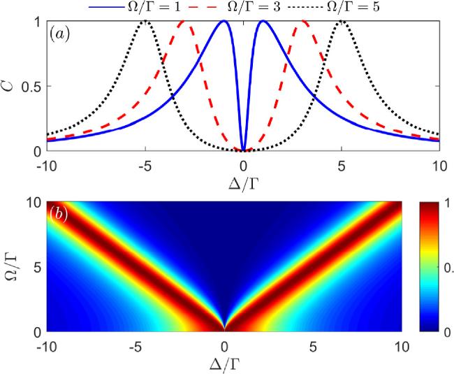
Figure 6. Contrast ratio C as a function of the detuning ${\rm{\Delta }}/{\rm{\Gamma }}$ for different Rabi frequencies in (a) and the corresponding contour map with respect to ${\rm{\Delta }}/{\rm{\Gamma }}$ and ${\rm{\Omega }}/{\rm{\Gamma }}$ in (b). Other common parameters are $\phi =\theta =\pi /2,$ ${{\rm{\Omega }}}_{2}=0$ and ${\gamma }_{e}=4{\rm{\Gamma }}$. |
Next, we turn our attention to the influence of the phase difference between the driving fields on the nonreciprocal scattering by taking the second driving field into account. We show the contrast ratio as a function of the detuning ${\rm{\Delta }}/{\rm{\Gamma }}$ and phase difference $\alpha $ under the conditions $\phi =\theta =\pi /2,$ ${{\rm{\Omega }}}_{2}={{\rm{\Omega }}}_{1}=3{\rm{\Gamma }}$ and ${\gamma }_{e}=4{\rm{\Gamma }}$ in figure 7(a), and the corresponding profiles of the contour map with different $\alpha $ in figure 7(b). From figure 7(a), one finds that the locations of the optimal nonreciprocal transmission windows and the corresponding separation between them can also be modified by adjusting the phase difference of the two driving fields with a period of $2\pi .$ As $\alpha $ increases from 0 to $2\pi ,$ the separation between the two optimal windows exhibits nonmonotonic variations based on $D=2\sqrt{{{\rm{\Omega }}}^{2}+{{\rm{\Gamma }}}^{2}{\sin }^{2}\theta {\cos }^{2}\phi }$ (corresponding to $D=6{\rm{\Gamma }}\sqrt{2\left(1+\,\cos \,\alpha \right)}$ in the present case).

Figure 7. Contrast ratio as a function of the detuning ${\rm{\Delta }}/{\rm{\Gamma }}$ and phase difference $\alpha $ in (a) and the corresponding profiles of the contour map with different $\alpha $ in (b). Other common parameters are $\phi =\theta =\pi /2,$ ${{\rm{\Omega }}}_{2}={{\rm{\Omega }}}_{1}=3{\rm{\Gamma }}$ and ${\gamma }_{e}=4{\rm{\Gamma }}$. |
As can be seen, when the driving fields are tuned in phase with $\alpha =0,$ there are two optimal transmission windows located at ${\rm{\Delta }}=\pm 6{\rm{\Gamma }}$ (with $D=12{\rm{\Gamma }}$), which can be seen more clearly in figure 7(b). As $\alpha $ increases in the region $\alpha \in \left(0,\pi \right),$ the separation becomes narrower with $D\lt 12{\rm{\Gamma }}.$ When the driving fields are tuned out of phase with $\alpha =\pi ,$ the two optimal windows will degenerate into a single one located at the resonant point due the perfect destructive interference between the two driving fields. By further increasing $\alpha $ from $\pi $ to $2\pi ,$ two optimal windows will appear again and the separation can be enlarged to $D=12{\rm{\Gamma }}$ when $\alpha =2\pi .$
In view of the above analysis, we find that the phase difference between the two driving fields can also function as a sensitive controller to manipulating the perfect nonreciprocal transmission, which provides an alternative way to achieve perfect nonreciprocal single-photon scattering. More interestingly, this is different from the single-field driving case, where one needs to turn off the driving field to realize perfect nonreciprocal transmission for the resonant photons. Here, perfect nonreciprocal transmission for photons with arbitrary frequencies within the region $-6{\rm{\Gamma }}\lt {\rm{\Delta }}\lt 6{\rm{\Gamma }},$ including the resonant photons with ${\rm{\Delta }}=0,$ is achievable by tuning the phase difference $\alpha $ while the two driving fields keep on turning. Theoretically, the effective frequency region for perfect nonreciprocal scattering can be further extended to the entire frequency range by accordingly increasing the Rabi frequencies of the two driving fields, as discussed in figure 6.
Before proceeding further, we want to point out that, other than the local coupling phases and driving phases, the accumulated phase between the two coupling points also plays an important role in realizing perfect nonreciprocal scattering. In figure 8, the upper plots are contour maps of the contrast ratio $C$ versus detuning ${\rm{\Delta }}/{\rm{\Gamma }}$ and accumulated phase $\theta ,$ while the middle ones depict the corresponding 2D profiles for some selected values of $\theta .$ We demonstrate the dependence of the nonreciprocal scattering on the accumulated phase in two special cases, i.e. $\alpha =0$ in figures 8(a) and (c), and $\alpha =\pi $ in figures 8(b) and (d) under the conditions $\phi =\pi /2,$ ${{\rm{\Omega }}}_{2}={{\rm{\Omega }}}_{1}=3{\rm{\Gamma }}$ and ${\gamma }_{e}=4{\rm{\Gamma }}.$ As can be seen, in both cases, the contrast ratio $C$ varies periodically with the accumulated phase $\theta $ with a period of $2\pi .$ When $\theta =\pi /2+n\pi ,$ a maximum of $C=\pm 1$ can be obtained, implying perfect nonreciprocal transmission. At the same time, $C\equiv 0$ when $\theta =n\pi ,$ which denotes the disappearance of the nonreciprocity. These results suggest that the nonreciprocal scattering can also be manipulated by modulating the accumulated phase between the two coupling points. However, different from that of the local coupling phases and the driving phases, here the location of the optimal nonreciprocal transmission window remains unchanged with the variation of $\theta .$ This is because, in the present cases, the locations of the optimal windows ${\rm{\Delta }}={\rm{\Gamma }}\,\sin \,\theta \,\cos \,\phi $ $\pm \sqrt{{{\rm{\Omega }}}^{2}+{{\rm{\Gamma }}}^{2}{\sin }^{2}\theta {\cos }^{2}\phi }$ are reduced to ${\rm{\Delta }}=\pm {\rm{\Omega }},$ which is independent of the accumulated phase.
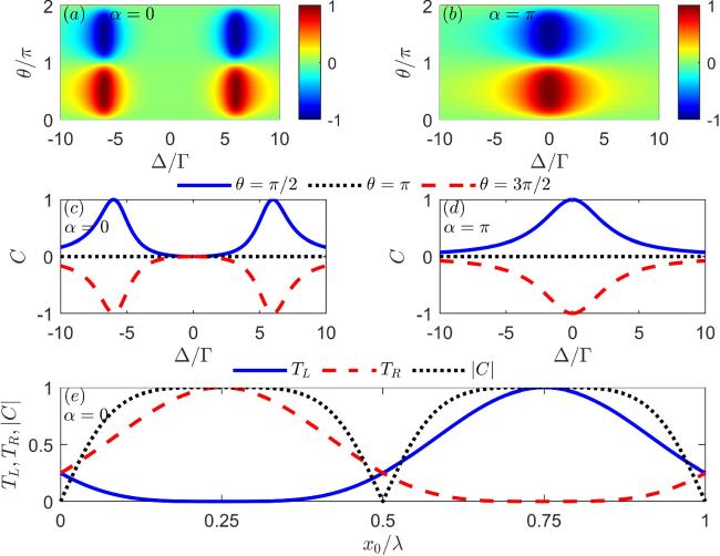
Figure 8. Contrast ratio $C$ versus detuning ${\rm{\Delta }}/{\rm{\Gamma }}$ and accumulated phase $\theta $ in (a) and (b), and the corresponding profiles of the contour map with different $\theta $ in (c) and (d). Transmission probabilities ${T}_{L},$ ${T}_{R}$ and the contrast ratio $\left|C\right|$ as a function of the distance between the two coupling points ${x}_{0}/\lambda $ with ${\rm{\Delta }}/{\rm{\Gamma }}=6$ in figure 8(e). Other common parameters are $\phi =\pi /2,$ ${{\rm{\Omega }}}_{2}={{\rm{\Omega }}}_{1}=3{\rm{\Gamma }}$ and ${\gamma }_{e}=4{\rm{\Gamma }}$. |
In order to intuitively show the influence of the separate distance between the two coupling points on the nonreciprocal single-photon scattering, in figure 8(e), we plot the transmission probabilities ${T}_{L},$ ${T}_{R}$ and the contrast ratio $\left|C\right|$ as a function of ${x}_{0}/\lambda ,$ where $\lambda $ is the wavelength of the inputting photons. It is clear from figure 8(e) that, when ${x}_{0}=n\lambda /2$ with $n=0,1,2\cdots ,$ the nonreciprocal transmission disappears with $\left|C\right|=0$ and the photons incident from both sides of the waveguide are reciprocally transmitted with equal probabilities ${T}_{L}={T}_{R}=0.25.$ However, for the case of ${x}_{0}\ne n\lambda /2,$ the nonreciprocal transmission occurs and perfect nonreciprocity $\left|C\right|=1$ can be achieved with ${T}_{L}=0,{T}_{R}=1$ or ${T}_{L}=1,{T}_{R}=0$ when ${x}_{0}=\left(2n+1\right)\lambda /4.$ These results agree well with those shown in figures 8(a)–(d), and the conditions for perfect nonreciprocal transmission here, i.e. ${x}_{0}=\left(2n+1\right)\lambda /4,$ corresponding to $\theta =\pi /2+n\pi $, as discussed above. This is because the accumulated phase $\theta $ and the separate distance ${x}_{0}$ between the two coupling points satisfy the relationship $\theta =k{x}_{0}=2\pi {x}_{0}/\lambda $ with $k=2\pi /\lambda .$
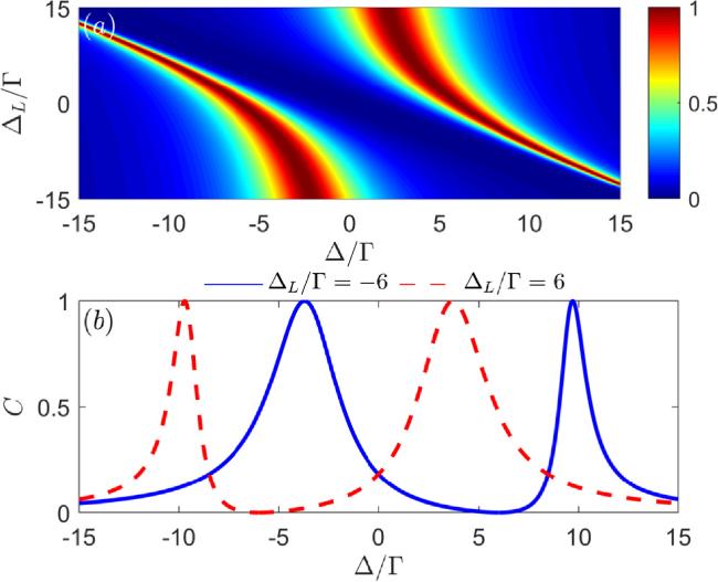
Finally, we explore how the driving detuning influences the nonreciprocal scattering. The contrast ratio $C$ as a function of the frequency detuning ${\rm{\Delta }}/{\rm{\Gamma }}$ and driving detuning ${{\rm{\Delta }}}_{L}$ under the conditions $\phi =\theta =\pi /2,$ $\alpha =0,$ ${{\rm{\Omega }}}_{2}={{\rm{\Omega }}}_{1}=3{\rm{\Gamma }}$ and ${\gamma }_{e}=4{\rm{\Gamma }}$ is plotted in figure 9(a), and the corresponding profiles of the contour map with different ${{\rm{\Delta }}}_{L}$ is shown in figure 9(b). It is found that the spectrum of $C$ displays two asymmetric peaks due to the driving detuning. Both the locations and widths of the peaks and dip can be modified by adjusting ${{\rm{\Delta }}}_{L}.$ When ${{\rm{\Delta }}}_{L}\gt 0,$ the spectrum shifts towards the left with a narrowed peak on the negative detuning side and a broadened one on the positive region, which are denoted by the two bright red zones in figure 9(a). This can be explained by the exact positions of the dip and the two peaks, which are expressed as ${{\rm{\Delta }}}_{{\rm{dip}}}=-{{\rm{\Delta }}}_{L}$ and ${{\rm{\Delta }}}_{{\rm{peak}}}=-{{\rm{\Delta }}}_{L}/2+{\rm{\Gamma }}\,\sin \,\theta \,\cos \,\phi $ $\pm \sqrt{{{\rm{\Omega }}}^{2}+{\left({{\rm{\Delta }}}_{L}/2+{\rm{\Gamma }}\,\sin \,\theta \,\cos \,\phi \right)}^{2}},$ respectively. As can be seen, for a fixed driving detuning ${{\rm{\Delta }}}_{L}=6{\rm{\Gamma }},$ the dip shifts to ${{\rm{\Delta }}}_{{\rm{dip}}}=-6{\rm{\Gamma }}$ and the two peaks shift to ${{\rm{\Delta }}}_{{\rm{peak}}}=-3{\rm{\Gamma }}\,\pm \sqrt{{{\rm{\Omega }}}^{2}+9{{\rm{\Gamma }}}^{2}}$ with a narrowed peak on the left and a broadened one on the right, as shown by the red dashed line in figure 9(b). As ${{\rm{\Delta }}}_{L}$ increases, especially when ${{\rm{\Delta }}}_{L}\gg {\rm{\Omega }},$ the peaks will further shift to ${{\rm{\Delta }}}_{{\rm{peak}}}\approx -{{\rm{\Delta }}}_{L}$ or $0,$ and the width of each peak can further narrow or broaden, as shown in figure 9(a). A similar analysis can be made to understand the variation of the spectrum within the region ${{\rm{\Delta }}}_{L}\lt 0.$ These remarkable properties may be useful for designing a single-photon diode with wide or narrow bandwidth based on demand.
Figure 9. Contrast ratio $C$ as a function of the frequency detuning ${\rm{\Delta }}/{\rm{\Gamma }}$ and driving detuning ${{\rm{\Delta }}}_{L}/{\rm{\Gamma }}$ in (a), and the corresponding profiles of the contour map with different ${{\rm{\Delta }}}_{L}$ in (b). Other common parameters are $\phi =\theta =\pi /2,$ $\alpha =0,$ ${{\rm{\Omega }}}_{2}={{\rm{\Omega }}}_{1}=3{\rm{\Gamma }}$ and ${\gamma }_{e}=4{\rm{\Gamma }}$. |
4. Conclusion
In summary, we have theoretically investigated the nonreciprocal single-photon scattering characteristics in a giant atom waveguide-QED system, which consists of a 1D waveguide and a three-level giant atom. The giant atom is configured as Λ-type, where one transition couples to the waveguide at two separate points, and the other is driven by two coherent driving fields. With the transmission probabilities of photons from two opposite sides, the contrast ratio used to describe the nonreciprocity is analytically derived, and the corresponding conditions for achieving perfect nonreciprocal transmission are obtained. We discussed, in detail, the nonreciprocal single-photon scattering characteristics in two cases, i.e. with or without the driven fields. The results reveal that, when the driving fields are turned off, an ideal diode for resonant photons with perfect contrast ratio can be achieved by tuning the local coupling phases between the giant atom and the waveguide. When the driving fields are turned on, a perfect frequency-tunable diode for photons with arbitrary frequencies can be realized by properly adjusting the Rabi frequencies and phase difference of the two extra driving fields. Different from the previous single-field driving schemes, here perfect nonreciprocal transmission for both resonant and non-resonant photons can be achieved without turning off the driving fields, which provides an alternative way to control the nonreciprocal single-photon scattering. Furthermore, the influence of the driving detuning on the nonreciprocal scattering is also discussed. It is found that the driving detuning plays an important role in manipulating the nonreciprocal single-photon scattering since a narrowed or broadened optimal nonreciprocal transmission window can be obtained by properly adjusting the driving detuning, which may be utilized to design single-photon diodes with wide or narrow bandwidth based on demand. The results in this paper may have potential applications in future quantum information processing with a giant atom setup.