


1. Introduction
Cold plasma is a material medium consisting of particles that vary in temperature. Cold plasma is not only a source of low-density electrons at room temperature and pressure, but also produces various reactive species when placed in a controlled environment. These reactive species are, in turn, useful in different chemical reactions in various fields of science. Consequently, plasma technology has become the subject of keen interest due to its manifold characteristics and low production costs.
Complete solutions of electromagnetic wave equations are known only for uniform or non-uniform regions and structures. A cylindrical waveguide is a uniform structure characterized by cross-sections transverse to the direction of propagation that are almost identical in size and shape to each other. Therefore, the electromagnetic field within such a waveguide can be presented as superposition of an infinite number of modes [1].
If the electromagnetic wave frequency delivered to the plasma surface is greater than the plasma frequency, the wave passes through it. However, if the frequency of the wave delivered to the plasma is lower than the plasma frequency, the wave does not pass through the plasma.
Plasma-filled waveguides are significant for the development of powerful microwave generators in optical systems and in the progress of high-power millimeter wave amplifiers, high information density communication, and as radio-frequency sources in accelerators for high-energy physics [2, 3]. The importance of collective plasma effects in a hollow-core target for achieving collimation of injected electrons and the impact of ion dynamics on laser-driven electron acceleration are also investigated [4, 5]. Note that the laser pulse transmits its energy to the plasma electrons, which can then be transformed into kinetic energy of other particles, including ions. In order to determine plasma and collision frequencies in the case of plasma or the dielectric constant and loss in the case of a dielectric, Thomassen [6] analyzed the interaction between a cylindrical plasma column (or dielectric material) and the resonant cavity from which it extends. Sakhnenko et al [7] gave analytical and numerical analysis of the electromagnetic fields of a circular cylinder of plasma with respect to time and spatial distribution. Alekhina and Tyukhtin [8] studied features of the Cherenkov-transition radiation generated in the vacuum area of a circular waveguide partly filled with strongly magnetized plasma. Electron acceleration and dynamics in plasma-filled rectangular, cylindrical, corrugated and elliptical waveguides have been a topic of interest in the past [9–12]. To investigate the impact of electron thermal velocity on the features of eigenmodes, Aghamir and Abbas-nejad [13] gave the numerical solution of the dispersion relations for these modes. Armaki et al [14] changed the plasma parameters of a coaxial waveguide to analyze their effect on the impedance, bandwidth, and the return losses. The absorption of a high-power millimeter pulse in a waveguide comprising plasma for a below critical density was established through simulations by Cao et al [15].
It is now evident that acceleration of particles can be carried out with the help of plasma, which supports very large electric fields. Intense lasers or particle beams [16] play a significant role in producing these fields. Therefore, these beams, particularly plasma beams, play a pivotal role in the advancement of astrophysics and energy production. Nusinovich et al [17] reviewed the development of hybrid modes in a slow-wave system containing plasma and the improvement of the coupling of the electromagnetic wave and plasma beam with the help of these modes. The advantages of implementing the asymmetric as well as symmetric eigenmodes of a slow electromagnetic wave within a traveling-wave tube were discussed by Abubakirov et al [18] in their paper. Carmel et al [19] concluded that a high-power microwave pulse is generated in a corrugated wall waveguide or a cylindrical wave tube when a relativistic electron beam passes. The dispersion features of a similar wave structure along with a helix-type slow-wave structure were analyzed by Hong-Quan and Pu-Kun [20, 21] for various geometric parameters and plasma densities. The relativistic traveling-wave tube and relativistic backward-wave oscillator work efficiently as amplifiers and high-power microwave sources. Bayat et al [22] found an exact numerical solution to the dispersion relation of these structures when they contain plasma and are powered by an electron beam.
Different numerical techniques have been applied to solve waveguide problems. A modal solution was found by Nguyen [23] for the associated waveguide problem inside an infinite cylindrical antenna. Applying the finite-difference time-domain method, Chaohui et al [24], numerically, made a 3D model of a rectangular waveguide used as a surface-wave plasma source. Ikuno et al [25] used the meshless time-domain method to evaluate the propagation of electromagnetic waves in various shaped waveguides. Abdoli-Arani and Moghaddasi [26] studied the acceleration of an electron injected inside a cylindrical waveguide having collisional plasma, using a mode-matching technique. Gashturi et al [27] suggested the employment of a combination of the method of moments and the mode-matching technique to numerically simulate the components of waveguides including cavity resonators.
It is apparent from the above discussion that although other numerical techniques along with the mode-matching method have been deployed for different types of slow-wave structures to study the electromagnetic phenomenon, the results were restricted to dispersion relations and electron dynamics. In this paper, we attempt to address the much-needed scattering characteristics, the orthogonality relation and power analysis in a plasma-filled cylindrical waveguide. The model presented can be applied as a traveling-wave tube containing uniform cold plasma in a cylindrical structure under the influence of a plasma beam.
The physical configuration of this cylindrical waveguide having a plasma beam embedded in cold and collisionless plasma is set out in section 2 . Section 3 provides the mode-matching solution of this slow-wave structure. Section 4 delivers the validity of the law of power conservation. Section 5 provides the detailed results obtained through numerical computations and considers their physical importance. The inference and deductions drawn from this analysis are presented in section 6 .
2. Formulation of waves propagating in a plasma beam embedded in a cold plasma environment
The wave problem investigated in this article revolves around scattering of electromagnetic waves in a cylindrical waveguide composed of a plasma beam immersed in cold plasma under the influence of a strong magnetic field. The scattering of electromagnetic waves is investigated within a metallic waveguide, which is depicted in figure 1. This infinite waveguide has a perfect electric conductor (PEC) boundary at r = a. The propagation of a TM incident wave is considered in a positive z direction from the left inlet z < 0 to the interface on the right. Being fundamental duct mode, this incident wave is presumed to have unit amplitude. The incident angle is zero with reference to the z axis. The region z < 0 comprises a vacuum and dielectric, as shown in the figure, with PEC walls placed at r = h1 and h2. The plasma beam in the right duct z > 0 is wrapped around by cold plasma at r = h1. The permittivity and permeability of vacuum are represented as ε0 and μ0, respectively. This configuration corresponds to a wavenumber k0 in the form ${k}_{0}\,=\,\omega \sqrt{{\mu }_{0}{\epsilon }_{0}}$, where ω represents the angular frequency and the speed of light c is related to free space permittivity and permeability as $c\,=\,1/\sqrt{{\epsilon }_{0}{\mu }_{0}}$. This association gives a new description to k0 expressed as k0 = ω/c. The permittivity εd in the dielectric medium is assumed to be εd = 2 × ε0. Therefore, the wavenumber in this medium can be manifested as ${k}_{1}\,=\,\sqrt{2}{k}_{0}.$ However, in the case of all media, i.e. beam, plasma and dielectric, the permeability remains μ0.
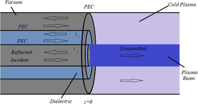
Figure 1. Propagation of electromagnetic waves in a cylindrical waveguide comprising a plasma beam embedded in cold plasma. |
A semi-finite intense and thick relativistic plasma beam of density nb, having a cold, collisionless, uniform plasma with density np, passes through the center of the waveguide. Here, the plasma and cyclotron frequencies are given, respectively, as ${\omega }_{p}\,=\,{\left({e}^{2}{n}_{p}/{\epsilon }_{0}m\right)}^{1/2}$ and ωc = eB0/m. These frequencies involve B0, m and e, which indicates the magnitude of magnetic field B0, electron mass and electric charge, respectively.
The permittivity tensor $\overline{\epsilon }$ [28, 29] , is,
$\begin{eqnarray}{\overline{\epsilon }}_{i}=\left[\begin{array}{ccc}{\epsilon }_{1} & -{\rm{i}}{\epsilon }_{2} & 0\\ {\rm{i}}{\epsilon }_{2} & {\epsilon }_{1} & 0\\ 0 & 0 & {\epsilon }_{3i}\end{array}\right],\end{eqnarray}$
where ${\epsilon }_{1}=1-\displaystyle \frac{{\omega }_{p}^{2}}{{\omega }^{2}-{\omega }_{c}^{2}},{\epsilon }_{2}=\displaystyle \frac{{\omega }_{c}{\omega }_{p}^{2}}{\omega \left({\omega }^{2}-{\omega }_{c}^{2}\right)}$.In order to refrain from the association of the TE and TM modes, B0 is considered to be very strong, so that ∣ε2∣ is infinitesimal and ε1 = 1 [30]. When i = b then ${\epsilon }_{3b}\,=1\,-\,\displaystyle \frac{{\omega }_{p}^{2}}{{\omega }^{2}}-\displaystyle \frac{{\omega }_{b}^{2}}{{\gamma }^{3}{(\omega -{k}_{{nz}}v)}^{2}}.$ These components form a tensor for the plasma beam. γ is the relativistic factor, knz = k0 + 2nπ, n = 0, 1, 2, …, is the axial wavenumber while v represents the beam velocity, so that $\gamma =\sqrt{1-\displaystyle \frac{{v}^{2}}{{c}^{2}}}.$ When i = p, then ${\epsilon }_{3p}=1-\displaystyle \frac{{\omega }_{p}^{2}}{{\omega }^{2}}.$ The tensor thus formed reveals the case of cold plasma. A time-independent variant e−iωt is considered but ignored throughout this paper [31].
Maxwell's equations govern the propagation of the electromagnetic waves in a waveguide. Faraday's law does not change for any of the four media, i.e. vacuum, dielectric, plasma beam and cold plasma.
$\begin{eqnarray}{\rm{\nabla }}\times {\boldsymbol{E}}={\rm{i}}\omega {\boldsymbol{B}}.\end{eqnarray}$
However, Ampere's law displays different behavior in each of these media and is discussed in the upcoming subsections.In the case of a 2D cylindrical waveguide, the fields remain invariant with respect to θ, i.e. ∂/∂θ = 0. For electromagnetic wave propagation, the Helmholtz equation derived from Maxwell's equations is solved along with boundary and interface conditions. The regions z < 0, 0 < r < h1, and z < 0, h2 < r < a contain a vacuum and are denoted by R1, R3, respectively. Likewise, R2 represents the region z < 0, h1 < r < h2 and contains a dielectric, R4 denotes the region z > 0, 0 < r < a, which encircles the plasma beam and the cold plasma.
2.1. Traveling-wave formulation in a vacuum
The formulation of Ampere's law in a vacuum is stated as,
$\begin{eqnarray}{\rm{\nabla }}\times {\boldsymbol{B}}=-\displaystyle \frac{{\rm{i}}\omega }{{c}^{2}}{\boldsymbol{E}}.\end{eqnarray}$
The Helmholtz equation in terms of longitudinal components is given as, $\begin{eqnarray}\left({{\rm{\nabla }}}^{2}+\displaystyle \frac{{\omega }^{2}}{{c}^{2}}\right)\left(\begin{array}{c}{E}_{z}\\ {B}_{z}\end{array}\right)=\left(\begin{array}{c}0\\ 0\end{array}\right).\end{eqnarray}$
The longitudinal components are the source to compute the following: $\begin{eqnarray*}{E}_{r}=\displaystyle \frac{{\rm{i}}s}{{\eta }^{2}}\displaystyle \frac{\partial {E}_{z}}{\partial r},\quad {E}_{\theta }=0,\end{eqnarray*}$
$\begin{eqnarray*}{B}_{r}=0,\quad {B}_{\theta }=\displaystyle \frac{{\rm{i}}\omega }{{c}^{2}{\eta }^{2}}\displaystyle \frac{\partial {E}_{z}}{\partial r},\end{eqnarray*}$
where, ${\eta }^{2}=\displaystyle \frac{{\omega }^{2}}{{c}^{2}}-{s}^{2}$ and s represents the wavenumber.The electric fields in regions R1 and R3 containing a vacuum, are expressed as φ1 and φ3, respectively.
The boundary conditions at the walls r = h1, h2 and a in region z < 0 are manifested a,4 ), the expansion of eigenfunctions is formed as follows:
$\begin{eqnarray}\displaystyle \frac{\partial {\phi }_{1}}{\partial r}({h}_{1},z)=0,\end{eqnarray}$
$\begin{eqnarray}\displaystyle \frac{\partial {\phi }_{3}}{\partial r}({h}_{2},z)=0,\end{eqnarray}$
$\begin{eqnarray}\displaystyle \frac{\partial {\phi }_{3}}{\partial r}(a,z)=0.\end{eqnarray}$
Applying the separation of variables technique to dimensional equation ( $\begin{eqnarray}{\phi }_{1}(r,z)=\displaystyle \sum _{n=0}^{\infty }{A}_{n}{{\rm{e}}}^{{\rm{i}}{s}_{n}^{(I)}(z)}{R}_{1n}^{(I)}(r),\end{eqnarray}$
$\begin{eqnarray}{\phi }_{3}(r,z)=\displaystyle \sum _{n=0}^{\infty }{C}_{n}{{\rm{e}}}^{{\rm{i}}{s}_{n}^{({III})}(z)}{R}_{1n}^{({III})}(r),\end{eqnarray}$
where An and Cn exhibit amplitudes in regions R1 and R3. The nth reflected modes in these regions of cylindrical waveguides have wavenumbers expressed as, ${s}_{n}^{(I)2}={k}_{0}^{2}-{\eta }_{n}^{2};\,{s}_{n}^{({III})2}\,={k}_{0}^{2}-{\lambda }_{n}^{2}.$The Bessel functions, in regions R1, are expressed as,6 ):5 ) and (7 ):
$\begin{eqnarray*}{R}_{1n}^{(I)}(r)={A}_{0}{J}_{0}({\eta }_{n}r),\end{eqnarray*}$
while in region R3, the Bessel functions take the following form after implementation of condition ( $\begin{eqnarray*}\begin{array}{l}{R}_{1n}^{({III})}(r)=\displaystyle \frac{{C}_{0}}{{N}_{0}^{{\prime} }({\lambda }_{n}{h}_{2})}\\ \quad \times \left\{{N}_{0}^{{\prime} }({\lambda }_{n}{h}_{2}){J}_{0}({\lambda }_{n}r)-{J}_{0}^{{\prime} }({\lambda }_{n}{h}_{2}){N}_{0}({\lambda }_{n}r)\right\}.\end{array}\end{eqnarray*}$
These functions satisfy the usual orthogonality relations in such a manner that, $\begin{eqnarray*}{E}_{1n}^{(I)}={\int }_{0}^{a}{R}_{1n}^{(I)2}(r)r{\rm{d}}r,\end{eqnarray*}$
$\begin{eqnarray*}{E}_{1n}^{({III})}={\int }_{{h}_{1}}^{{h}_{2}}{R}_{1n}^{({III})2}(r)r{\rm{d}}r.\end{eqnarray*}$
It is important to note that ηn and λn; n = 0, 1, 2, … are the roots of the equations derived from boundary conditions ( $\begin{eqnarray}{J}_{0}^{{\prime} }({\eta }_{n}{h}_{1})=0,\end{eqnarray}$
$\begin{eqnarray}{N}_{0}^{{\prime} }({\lambda }_{n}{h}_{2}){J}_{0}^{{\prime} }({\lambda }_{n}a)-{J}_{0}^{{\prime} }({\lambda }_{n}{h}_{2}){N}_{0}^{{\prime} }({\lambda }_{n}a)=0.\end{eqnarray}$
2.2. Traveling-wave formulation in a dielectric medium
The dielectrics are governed by Ampere's law in the following manner:
$\begin{eqnarray}{\rm{\nabla }}\times {\boldsymbol{B}}=-{\rm{i}}\omega {\epsilon }_{d}{\mu }_{0}{\boldsymbol{E}}.\end{eqnarray}$
The Helmholtz equation for the electromagnetic waves propagating in a dielectric medium, can be indicated in longitudinal components as, $\begin{eqnarray}\left({{\rm{\nabla }}}^{2}+{\omega }^{2}{\epsilon }_{d}{\mu }_{0}\right)\left(\begin{array}{c}{E}_{z}\\ {B}_{z}\end{array}\right)=\left(\begin{array}{c}0\\ 0\end{array}\right).\end{eqnarray}$
The transverse components can be stated as, $\begin{eqnarray*}{E}_{r}=\displaystyle \frac{{\rm{i}}s}{{\tau }^{2}}\displaystyle \frac{\partial {E}_{z}}{\partial r},\quad {E}_{\theta }=0,\end{eqnarray*}$
$\begin{eqnarray*}{B}_{r}=0,\quad {B}_{\theta }=\displaystyle \frac{{\rm{i}}{k}_{1}^{2}}{\omega {\tau }^{2}}\displaystyle \frac{\partial {E}_{z}}{\partial r},\end{eqnarray*}$
so that ${\tau }^{2}={k}_{1}^{2}-{s}^{2},$ where ${k}_{1}^{2}={\omega }^{2}{\epsilon }_{d}{\mu }_{0}.$The boundary conditions at the walls in the dielectric region are exhibited as,13 ), the eigenfunction expansion takes the following form:
$\begin{eqnarray}\displaystyle \frac{\partial {\phi }_{2}}{\partial r}({h}_{1},z)=0,\end{eqnarray}$
$\begin{eqnarray}\displaystyle \frac{\partial {\phi }_{2}}{\partial r}({h}_{2},z)=0.\end{eqnarray}$
Incorporating the method of separation of variables to dimensional equation ( $\begin{eqnarray}{\phi }_{2}(r,z)=\displaystyle \sum _{n=0}^{\infty }{B}_{n}{{\rm{e}}}^{{\rm{i}}{s}_{n}^{({II})}z}{R}_{1n}^{({II})}(r),\end{eqnarray}$
where Bn denote the amplitudes in regions R2. The wavenumber of the nth mode is given as ${s}_{n}^{({II})2}={\omega }^{2}{\epsilon }_{d}{\mu }_{0}-{\tau }_{n}^{2}.$Boundary condition (14 ) yields the Bessel functions, in this region, as,17 ) derived from boundary condition (15 ) are given as τn; n = 0, 1, 2,…,
$\begin{eqnarray*}{R}_{2n}^{({II})}(r)=\displaystyle \frac{{B}_{0}}{{N}_{0}^{{\prime} }({\tau }_{n}{h}_{1})}\left\{{N}_{0}^{{\prime} }({\tau }_{n}{h}_{1}){J}_{0}({\tau }_{n}r)-{J}_{0}^{{\prime} }({\tau }_{n}{h}_{2}){N}_{0}({\tau }_{n}r)\right\},\end{eqnarray*}$
which satisfy the usual orthogonality relations, so that, $\begin{eqnarray*}{E}_{1n}^{({II})}={\int }_{0}^{{h}_{1}}{R}_{1n}^{({II})2}(r)r{\rm{d}}r.\end{eqnarray*}$
The roots of equation ( $\begin{eqnarray}{N}_{0}^{{\prime} }({\tau }_{n}{h}_{2}){J}_{0}^{{\prime} }({\tau }_{n}a)-{J}_{0}^{{\prime} }({\tau }_{n}{h}_{2}){N}_{0}^{{\prime} }({\tau }_{n}a)=0.\end{eqnarray}$
2.3. Traveling-wave formulation in a plasma beam and cold plasma
Ampere's law for a plasma beam is of the following form:
$\begin{eqnarray}{\rm{\nabla }}\times {\boldsymbol{B}}=-\displaystyle \frac{{\rm{i}}\omega }{{c}^{2}}{\overline{\epsilon }}_{b}.{\boldsymbol{E}}.\end{eqnarray}$
The Helmholtz equation, in the case of propagation of a plasma beam, stated in longitudinal components: $\begin{eqnarray*}\begin{array}{l}\left\{{{\rm{\nabla }}}^{2}+\left(\displaystyle \frac{{\omega }^{2}}{{c}^{2}}-{k}_{{nz}}^{2}\right)\left(1-\displaystyle \frac{{\omega }_{p}^{2}}{{\omega }^{2}}-\displaystyle \frac{{\omega }_{b}^{2}}{{\gamma }^{3}{\left(\omega -{k}_{{nz}}v\right)}^{2}}\right)\right\}\\ \,\times \left(\begin{array}{c}{E}_{z}\\ {B}_{z}\end{array}\right)\,=\,\left(\begin{array}{c}0\\ 0\end{array}\right),\end{array}\end{eqnarray*}$
is transformed into the equation: $\begin{eqnarray}\left({{\rm{\nabla }}}^{2}+{T}_{1}^{2}\right)\left(\begin{array}{c}{E}_{z}\\ {B}_{z}\end{array}\right)=\left(\begin{array}{c}0\\ 0\end{array}\right),\end{eqnarray}$
where ${T}_{1}^{2}=\left(\displaystyle \frac{{\omega }^{2}}{{c}^{2}}-{k}_{{nz}}^{2}\right)\left(1-\displaystyle \frac{{\omega }_{p}^{2}}{{\omega }^{2}}-\displaystyle \frac{{\omega }_{b}^{2}}{{\gamma }^{3}{\left(\omega -{k}_{{nz}}v\right)}^{2}}\right).$The transverse components can be given as,
$\begin{eqnarray*}{E}_{r}=\displaystyle \frac{{\rm{i}}s}{{\chi }^{2}}\displaystyle \frac{\partial {E}_{z}}{\partial r},\quad {E}_{\theta }=0,\end{eqnarray*}$
$\begin{eqnarray*}{B}_{r}=0,\quad {B}_{\theta }=\displaystyle \frac{{\rm{i}}{T}_{1}^{2}}{\omega {\chi }^{2}}\displaystyle \frac{\partial {E}_{z}}{\partial r}.\end{eqnarray*}$
Here, ${\chi }^{2}={T}_{1}^{2}-{s}^{2}$.Ampere's law for cold plasma is formulated as,
$\begin{eqnarray}{\rm{\nabla }}\times {\boldsymbol{B}}=-\displaystyle \frac{{\rm{i}}\omega }{{c}^{2}}{\overline{\epsilon }}_{p}.{\boldsymbol{E}}.\end{eqnarray}$
For propagation in cold plasma [32], the Helmholtz equation in terms of longitudinal components, is as follows: $\begin{eqnarray*}\left\{{{\rm{\nabla }}}^{2}+\left(\displaystyle \frac{{\omega }^{2}}{{c}^{2}}-{k}_{{nz}}^{2}\right)\left(1-\displaystyle \frac{{\omega }_{p}^{2}}{{\omega }^{2}}\right)\right\}\left(\begin{array}{c}{E}_{z}\\ {B}_{z}\end{array}\right)=\left(\begin{array}{c}0\\ 0\end{array}\right),\end{eqnarray*}$
which can be further transformed as, $\begin{eqnarray}\left({{\rm{\nabla }}}^{2}+{T}_{2}^{2}\right)\left(\begin{array}{c}{E}_{z}\\ {B}_{z}\end{array}\right)=\left(\begin{array}{c}0\\ 0\end{array}\right),\end{eqnarray}$
where ${T}_{2}^{2}=\left(\displaystyle \frac{{\omega }^{2}}{{c}^{2}}-{k}_{{nz}}^{2}\right)\left(1-\displaystyle \frac{{\omega }_{p}^{2}}{{\omega }^{2}}\right).$The transverse components of the field can be revealed as,
$\begin{eqnarray*}{E}_{r}=\displaystyle \frac{{\rm{i}}s}{{\gamma }^{2}}\displaystyle \frac{\partial {E}_{z}}{\partial r},\quad {E}_{\theta }=0,\end{eqnarray*}$
$\begin{eqnarray*}{B}_{r}=0,\quad {B}_{\theta }=\displaystyle \frac{{\rm{i}}{T}_{2}^{2}}{\omega {\gamma }^{2}}\displaystyle \frac{\partial {E}_{z}}{\partial r},\end{eqnarray*}$
where ${\gamma }^{2}={T}_{2}^{2}-{s}^{2}$.The boundary conditions at the walls r = h1 and a in this region are mentioned as,19 ) and (21 ), yields the eigenfunction expansion as,
$\begin{eqnarray}{\phi }_{4}^{(I)}({h}_{1},z)={\phi }_{4}^{({II})}({h}_{1},z),\end{eqnarray}$
$\begin{eqnarray}\displaystyle \frac{\partial {\phi }_{4}^{(I)}}{\partial r}({h}_{1},z)=\displaystyle \frac{\partial {\phi }_{4}^{({II})}}{\partial r}({h}_{1},z),\end{eqnarray}$
$\begin{eqnarray}\displaystyle \frac{\partial {\phi }_{4}^{({II})}}{\partial r}(a,z)=0.\end{eqnarray}$
Employing the variable separable technique to equation ( $\begin{eqnarray}\begin{array}{l}{\phi }_{4}(r,z)=\,\left\{\begin{array}{ll}{\phi }_{4}^{(I)}(r,z), & 0\lt r\lt {h}_{1},\\ {\phi }_{4}^{({II})}(r,z), & {h}_{1}\lt r\lt a.\end{array}\right.\\ \,=\,\left\{\begin{array}{ll}\displaystyle \sum _{n=0}^{\infty }{D}_{n}{{\rm{e}}}^{{\rm{i}}{s}_{n}z}{R}_{2n}^{(I)}(r), & 0\lt r\lt {h}_{1},\\ \displaystyle \sum _{n=0}^{\infty }{D}_{n}{{\rm{e}}}^{{\rm{i}}{s}_{n}z}{R}_{2n}^{({II})}(r), & {h}_{1}\lt r\lt a,\end{array}\right.\end{array}\end{eqnarray}$
where Dn represent the amplitudes in regions R4 and sn; n = 0, 1, 2, … reveals the wavenumber of the nth mode.The Bessel functions, in this region, are expressed as,22 ) and (23 ),
$\begin{eqnarray*}{R}_{2n}^{(I)}(r)={D}_{0}{J}_{0}({\chi }_{n}r),\end{eqnarray*}$
$\begin{eqnarray*}{R}_{2n}^{({II})}(r)=\displaystyle \frac{{E}_{0}}{{N}_{0}^{{\prime} }({\gamma }_{n}a)}\left\{{N}_{0}^{{\prime} }({\gamma }_{n}a){J}_{0}({\gamma }_{n}r)-{J}_{0}^{{\prime} }({\gamma }_{n}a){N}_{0}({\gamma }_{n}r)\right\}.\end{eqnarray*}$
The Bessel functions in z > 0, satisfy the derived orthogonality relation: $\begin{eqnarray}{\int }_{0}^{{h}_{1}}{R}_{2m}^{(I)}(r){R}_{2n}^{(I)}(r)r{\rm{d}}r+{\int }_{{h}_{1}}^{a}{R}_{2m}^{({II})}(r){R}_{2n}^{({II})}(r)r{\rm{d}}r={\delta }_{{mn}}{E}_{m},\end{eqnarray}$
where $\begin{eqnarray*}{E}_{n}={\int }_{0}^{{h}_{1}}{R}_{2n}^{(I)2}(r)r{\rm{d}}r+{\int }_{{h}_{1}}^{a}{R}_{2n}^{({II})2}(r)r{\rm{d}}r.\end{eqnarray*}$
Here, ${\chi }_{n}^{2}={T}_{1}^{2}-{s}_{n}^{2}$ and ${\gamma }_{n}^{2}={T}_{2}^{2}-{s}_{n}^{2};\,n=0,1,2,\ldots $ are the roots of the equation derived from boundary conditions ( $\begin{eqnarray}\begin{array}{l}\quad {\chi }_{n}\left\{{J}_{0}^{{\prime} }({\chi }_{n}{h}_{1}){N}_{0}^{{\prime} }({\gamma }_{n}a){J}_{0}({\gamma }_{n}{h}_{1})-{J}_{0}^{{\prime} }({\chi }_{n}{h}_{1}){J}_{0}^{{\prime} }({\gamma }_{n}a){N}_{0}({\gamma }_{n}{h}_{1})\right\}\\ =\,{\gamma }_{n}\left\{{N}_{0}^{{\prime} }({\gamma }_{n}a){J}_{0}^{{\prime} }({\gamma }_{n}{h}_{1}){J}_{0}({\chi }_{n}{h}_{1})-{J}_{0}^{{\prime} }({\gamma }_{n}a){N}_{0}^{{\prime} }({\gamma }_{n}{h}_{1}){J}_{0}({\chi }_{n}{h}_{1})\right\}.\end{array}\end{eqnarray}$
2.4. Matching conditions
Since the fields are continuous at the interface z = 0, the following matching conditions exist:
$\begin{eqnarray}{\phi }_{1}(r,0)={\phi }_{4}^{(I)}(r,0),\quad 0\leqslant r\leqslant {h}_{1},\end{eqnarray}$
$\begin{eqnarray}{\phi }_{2}(r,0)={\phi }_{4}^{({II})}(r,0),\quad {h}_{1}\leqslant r\leqslant {h}_{2},\end{eqnarray}$
$\begin{eqnarray}{\phi }_{3}(r,0)={\phi }_{4}^{({II})}(r,0),\quad {h}_{2}\leqslant r\leqslant a,\end{eqnarray}$
$\begin{eqnarray}\displaystyle \frac{\partial {\phi }_{1}}{\partial z}(r,0)=\displaystyle \frac{\partial {\phi }_{4}^{(I)}}{\partial z}(r,0),\quad 0\leqslant r\leqslant {h}_{1},\end{eqnarray}$
$\begin{eqnarray}\displaystyle \frac{\partial {\phi }_{2}}{\partial z}(r,0)=\displaystyle \frac{\partial {\phi }_{4}^{({II})}}{\partial z}(r,0),\quad {h}_{1}\leqslant r\leqslant {h}_{2},\end{eqnarray}$
$\begin{eqnarray}\displaystyle \frac{\partial {\phi }_{1}}{\partial z}(r,0)=\displaystyle \frac{\partial {\phi }_{4}^{({II})}}{\partial z}(r,0).\quad {h}_{2}\leqslant r\leqslant a.\end{eqnarray}$
3. Mode-matching solution
From conditions (28 )–(30 ), we have the following:34 ) by ${R}_{1m}^{(I)}(r)r$ and integrating from 0 to h1, we obtain:35 ) and (36 ) produce the following:31 )–(33 ) and solving in the above-mentioned manner, the following equations are formed:40 ) by ${R}_{2m}^{(I)}(r)r$ and integrating from 0 to h1, yields the following:41 ) and (42 ) by ${R}_{2m}^{({II})}(r)r$ and integrating from h1 to a, the following equation is formed:43 ) and (44 ) and employing the derived orthogonality relation (26 ) , we obtain:37 )–(39 ) and (45 ) having the unknown coefficients $\left\{{A}_{n},{B}_{n},{C}_{n},{D}_{n}\right\},\,n=0,1,2,\ldots $ The system is solved numerically after truncation and the outcomes are displayed and scrutinized in the numerical section.
$\begin{eqnarray}1+\displaystyle \sum _{n=0}^{\infty }{A}_{n}{R}_{1n}^{(I)}(r)=\displaystyle \sum _{n=0}^{\infty }{D}_{n}{R}_{2n}^{(I)}(r),\end{eqnarray}$
$\begin{eqnarray}1+\displaystyle \sum _{n=0}^{\infty }{B}_{n}{R}_{1n}^{({II})}(r)=\displaystyle \sum _{n=0}^{\infty }{D}_{n}{R}_{2n}^{({II})}(r),\end{eqnarray}$
$\begin{eqnarray}1+\displaystyle \sum _{n=0}^{\infty }{C}_{n}{R}_{1n}^{({III})}(r)=\displaystyle \sum _{n=0}^{\infty }{D}_{n}{R}_{2n}^{({II})}(r).\end{eqnarray}$
Multiplying both sides of ( $\begin{eqnarray}{A}_{m}=-{\delta }_{m0}+\frac{1}{{E}_{1m}^{(I)}}\displaystyle \sum _{n=0}^{\infty }{D}_{n}{P}_{{mn}},\end{eqnarray}$
where $\begin{eqnarray*}{P}_{{mn}}={\int }_{0}^{{h}_{1}}{R}_{1m}^{(I)}(r){R}_{2n}^{(I)}(r)r{\rm{d}}r.\end{eqnarray*}$
Solving in a similar manner, equations ( $\begin{eqnarray}{B}_{m}=-{\delta }_{m0}+\frac{1}{{E}_{1m}^{({II})}}\displaystyle \sum _{n=0}^{\infty }{D}_{n}{Q}_{{mn}},\end{eqnarray}$
$\begin{eqnarray}{C}_{m}=-{\delta }_{m0}+\frac{1}{{E}_{1m}^{({III})}}\displaystyle \sum _{n=0}^{\infty }{D}_{n}{R}_{{mn}},\end{eqnarray}$
where $\begin{eqnarray*}{Q}_{{mn}}={\int }_{{h}_{1}}^{{h}_{2}}{R}_{1m}^{({II})}(r){R}_{2n}^{({II})}(r)r{\rm{d}}r,\end{eqnarray*}$
$\begin{eqnarray*}{R}_{{mn}}={\int }_{{h}_{2}}^{a}{R}_{1m}^{({III})}(r){R}_{2n}^{({II})}(r)r{\rm{d}}r.\end{eqnarray*}$
Now, incorporating conditions ( $\begin{eqnarray}{k}_{0}-\displaystyle \sum _{n=0}^{\infty }{A}_{n}{s}_{n}^{(I)}{R}_{1n}^{(I)}(r)=\displaystyle \sum _{n=0}^{\infty }{D}_{n}{s}_{n}{R}_{2n}^{(I)}(r),\end{eqnarray}$
$\begin{eqnarray}{k}_{1}-\displaystyle \sum _{n=0}^{\infty }{B}_{n}{s}_{n}^{({II})}{R}_{1n}^{({II})}(r)=\displaystyle \sum _{n=0}^{\infty }{D}_{n}{s}_{n}{R}_{2n}^{({II})}(r),\end{eqnarray}$
$\begin{eqnarray}{k}_{0}-\displaystyle \sum _{n=0}^{\infty }{C}_{n}{s}_{n}^{({III})}{R}_{1n}^{({III})}(r)=\displaystyle \sum _{n=0}^{\infty }{D}_{n}{s}_{n}{R}_{2n}^{({II})}(r).\end{eqnarray}$
Multiplying ( $\begin{eqnarray}{k}_{0}{P}_{0m}-\displaystyle \sum _{n=0}^{\infty }{A}_{n}{s}_{n}^{(I)}{P}_{{nm}}=\displaystyle \sum _{n=0}^{\infty }{D}_{n}{s}_{n}{\int }_{0}^{{h}_{1}}{R}_{2m}^{(I)}{R}_{2n}^{(I)}(r)r{\rm{d}}r.\end{eqnarray}$
Similarly, multiplying ( $\begin{eqnarray}\begin{array}{r}{k}_{1}{Q}_{0m}+{k}_{0}{R}_{0m}-\displaystyle \sum _{n=0}^{\infty }{B}_{n}{s}_{n}^{({II})}{Q}_{{nm}}-\displaystyle \sum _{n=0}^{\infty }{C}_{n}{s}_{n}^{({III})}{R}_{{nm}}\\ =\,\displaystyle \sum _{n=0}^{\infty }{D}_{n}{s}_{n}{\displaystyle \int }_{{h}_{1}}^{a}{R}_{2m}^{({II})}{R}_{2n}^{({II})}(r)r{\rm{d}}r.\end{array}\end{eqnarray}$
Adding ( $\begin{eqnarray}\begin{array}{rcl}{D}_{m} & = & \displaystyle \frac{1}{{s}_{m}{E}_{m}}\left({k}_{0}{P}_{0m}-\displaystyle \sum _{n=0}^{\infty }{A}_{n}{s}_{n}^{(I)}{P}_{{nm}}\right)+\displaystyle \frac{1}{{s}_{m}{E}_{m}}\\ & & \times \,\left({k}_{1}{Q}_{0m}+{k}_{0}{R}_{0m}-\displaystyle \sum _{n=0}^{\infty }{B}_{n}{s}_{n}^{({II})}{Q}_{{nm}}-\displaystyle \sum _{n=0}^{\infty }{C}_{n}{s}_{n}^{({III})}{R}_{{nm}}\right).\end{array}\end{eqnarray}$
A system of infinite equations is manifested through equations (4. Energy flux
The energy flux is a yardstick that determines the convergence of the truncated solution and its accuracy.
The Poynting vector is utilized to find energy propagating in different sections of the waveguide, which is stated as [33],
$\begin{eqnarray}\mathrm{Power}={\int }_{R}\pi r\mathrm{Re}\left\{{E}_{z}{\left(\displaystyle \frac{\partial {E}_{z}}{\partial z}\right)}^{* }\right\}{\rm{d}}r,\end{eqnarray}$
where (*) represents a complex conjugate.Since we have three different regions in the left duct z < 0, the incident and reflected powers in this duct are of the form:52 ) as,
$\begin{eqnarray}{P}_{i}={P}_{i}^{(I)}+{P}_{i}^{({II})}+{P}_{i}^{({III})},\end{eqnarray}$
$\begin{eqnarray}{P}_{r}={P}_{r}^{(I)}+{P}_{r}^{({II})}+{P}_{r}^{({III})}.\end{eqnarray}$
By employing the Poynting vector, the incident (Pi), reflected (Pr) and transmitted (Pt) powers can be ascertained as, $\begin{eqnarray}{P}_{i}=\displaystyle \frac{\pi {k}_{0}{h}_{1}^{2}}{2}+\displaystyle \frac{\pi {k}_{1}({h}_{2}^{2}-{h}_{1}^{2})}{2}+\displaystyle \frac{\pi {k}_{0}({a}^{2}-{h}_{2}^{2})}{2},\end{eqnarray}$
$\begin{eqnarray}\begin{array}{rcl}{P}_{r} & = & -\pi \mathrm{Re}\left(\displaystyle \sum _{n=0}^{\infty }| {A}_{n}{| }^{2}{s}_{n}^{(I)}{E}_{1n}^{(I)}\right)-\pi \mathrm{Re}\left(\displaystyle \sum _{n=0}^{\infty }| {B}_{n}{| }^{2}{s}_{n}^{({II})}{E}_{1n}^{({II})}\right)\\ & & -\pi \mathrm{Re}\left(\displaystyle \sum _{n=0}^{\infty }| {C}_{n}{| }^{2}{s}_{n}^{({III})}{E}_{1n}^{({III})}\right),\end{array}\end{eqnarray}$
$\begin{eqnarray}{P}_{t}=\pi \mathrm{Re}\left(\displaystyle \sum _{n=0}^{\infty }| {D}_{n}{| }^{2}{s}_{n}{E}_{n}\right).\end{eqnarray}$
The application of the law of conservation of power, $\begin{eqnarray*}{P}_{i}+{P}_{r}={P}_{t}\end{eqnarray*}$
yields the following form, $\begin{eqnarray}\begin{array}{l}\displaystyle \frac{\pi {k}_{0}{h}_{1}^{2}}{2}+\displaystyle \frac{\pi {k}_{1}({h}_{2}^{2}-{h}_{1}^{2})}{2}+\displaystyle \frac{\pi {k}_{0}({a}^{2}-{h}_{2}^{2})}{2}\\ -\pi \mathrm{Re}\left(\displaystyle \sum _{n=0}^{\infty }| {A}_{n}{| }^{2}{s}_{n}^{(I)}{E}_{1n}^{(I)}\right)-\pi \mathrm{Re}\left(\displaystyle \sum _{n=0}^{\infty }| {B}_{n}{| }^{2}{s}_{n}^{({II})}{E}_{1n}^{({II})}\right)\\ -\pi \mathrm{Re}\left(\displaystyle \sum _{n=0}^{\infty }| {C}_{n}{| }^{2}{s}_{n}^{({III})}{E}_{1n}^{({III})}\right)=\pi \mathrm{Re}\left(\displaystyle \sum _{n=0}^{\infty }| {D}_{n}{| }^{2}{s}_{n}{E}_{n}\right).\end{array}\end{eqnarray}$
The incident power Pi is scaled to unity to reshape equation ( $\begin{eqnarray}1={{ \mathcal E }}_{1}+{{ \mathcal E }}_{2}+{{ \mathcal E }}_{3}+{{ \mathcal E }}_{4},\end{eqnarray}$
where $\begin{eqnarray}\begin{array}{l}{{ \mathcal E }}_{1}=\displaystyle \frac{2}{K}\mathrm{Re}\left(\displaystyle \sum _{n=0}^{\infty }| {A}_{n}{| }^{2}{s}_{n}^{(I)}{E}_{1n}^{(I)}\right),\end{array}\end{eqnarray}$
$\begin{eqnarray}\begin{array}{l}{{ \mathcal E }}_{2}=\displaystyle \frac{2}{K}\mathrm{Re}\left(\displaystyle \sum _{n=0}^{\infty }| {B}_{n}{| }^{2}{s}_{n}^{({II})}{E}_{1n}^{({II})}\right),\end{array}\end{eqnarray}$
$\begin{eqnarray}\begin{array}{l}{{ \mathcal E }}_{3}=\displaystyle \frac{2}{K}\mathrm{Re}\left(\displaystyle \sum _{n=0}^{\infty }| {C}_{n}{| }^{2}{s}_{n}^{({III})}{E}_{1n}^{({III})}\right),\end{array}\end{eqnarray}$
$\begin{eqnarray}\begin{array}{l}{{ \mathcal E }}_{4}=\displaystyle \frac{2}{K}\mathrm{Re}\left(\displaystyle \sum _{n=0}^{\infty }| {D}_{n}{| }^{2}{s}_{n}{E}_{n}\right),\end{array}\end{eqnarray}$
and $\begin{eqnarray*}K={k}_{0}{h}_{1}^{2}+{k}_{1}({h}_{2}^{2}-{h}_{1}^{2})+{k}_{0}({a}^{2}-{h}_{2}^{2}).\end{eqnarray*}$
5. Numerical results and discussion
The results of numerical solutions of the given physical problem are furnished in this section. The electric fields are presented in the figures as follows:
$\begin{eqnarray*}{\phi }_{T}(r,z)=\left\{\begin{array}{lr}{\phi }_{1}(r,z),\quad z\lt 0, & 0\lt r\lt {h}_{1},\\ {\phi }_{2}(r,z),\quad z\lt 0, & {h}_{1}\lt r\lt {h}_{2},\\ {\phi }_{3}(r,z),\quad z\lt 0, & {h}_{2}\lt r\lt a,\\ {\phi }_{4}(r,z),\quad z\gt 0, & 0\lt r\lt a.\end{array}\right.\end{eqnarray*}$
The magnetic fields in the respective regions are displayed in the figures in the following manner: $\begin{eqnarray*}{\phi }_{{Tx}}(r,z)=\left\{\begin{array}{lr}{\phi }_{1z}(r,z),\quad z\lt 0, & 0\lt r\lt {h}_{1},\\ {\phi }_{2z}(r,z),\quad z\lt 0, & {h}_{1}\lt r\lt {h}_{2},\\ {\phi }_{3z}(r,z),\quad z\lt 0, & {h}_{2}\lt r\lt a,\\ {\phi }_{4z}(r,z),\quad z\gt 0, & 0\lt r\lt a,\end{array}\right.\end{eqnarray*}$
where $\phi {jz}=\displaystyle \frac{\partial {\phi }_{i}}{\partial z};j=1,2,3,4.$The physical parameters chosen are the speed of light, c = 3 × 10⁸ m s−1, permittivity and permeability of free space, expressed respectively, as ε0 = 8.85 × 10⁻¹² farad m–1 and μ0 = 4π × 10−7 N/A2(Newtons per Ampere squared). To obtain rigorous numerical results, the duct radii are set as ${\overline{h}}_{1}=0.2$ cm, ${\overline{h}}_{2}=0.3$ cm and $\overline{a}=0.4$ cm. The beam velocity v is fixed at 0.134 × 108 cm s–1, while the frequencies are taken as ω = 2.5 × 10⁹ rad s−1, ωb = 2 × 10⁹ rad s−1 and ωp = 109 rad s−1. The axial wavenumber is considered to be k1z = k0 + 2π. The quantities h1, h2 and a reveal the non-dimensional form of radii ${\overline{h}}_{1},{\overline{h}}_{2}$ and $\overline{a},$ respectively. The software Mathematica (version 12.1) is used to carry out the simulations.
The mode-matching solution of the system revealed in equations (37 ), (38 ), (39 ) and (45 ) with a truncation parameter N is applied to obtain the numerical results. The solution yields the unknowns $\left\{{A}_{n},{B}_{n},{C}_{n},{D}_{n}\right\};\,n=0,1,2,\ldots ,149$ and is utilized to exhibit the accuracy of algebra, distribution of energy and its conservation.
Figures 2– 7 confirm that the matching conditions are validated by the solution at the interface z = 0. In all media, i.e. vacuum, dielectric, beam and cold plasma, the graphs of magnetic and electric fields reveal that the real and imaginary parts are in excellent agreement along with the interface.
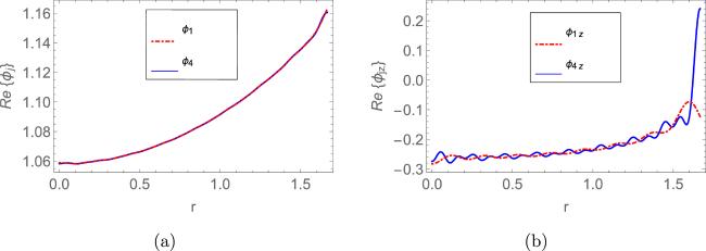
Figure 2. Real parts of the electric field and magnetic fields at the interface z = 0 and 0 ≤ r ≤ h1. |
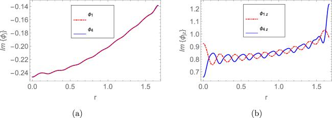
Figure 3. Imaginary parts of the electric field and magnetic fields at the interface z = 0 and 0 ≤ r ≤ h1. |

Figure 4. Real parts of the electric field and magnetic fields at the interface z = 0 and h1 ≤ r ≤ h2. |
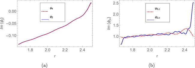
Figure 5. Imaginary parts of the electric field and magnetic fields at the interface z = 0 and h1 ≤ r ≤ h2. |

Figure 6. Real parts of the electric field and magnetic fields at the interface z = 0 and h2 ≤ r ≤ a. |
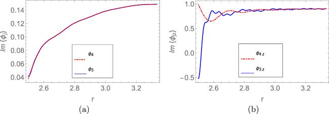
Figure 7. Imaginary parts of the electric field and magnetic fields at the interface z = 0 and h2 ≤ r ≤ a. |
The cogency of the law of power conservation in different duct regions is another check on the accuracy of the truncated solution. The reflected powers in left duct (z < 0) for regions R1, R2 and R3 are represented by ${{ \mathcal E }}_{1},{{ \mathcal E }}_{2}$ and ${{ \mathcal E }}_{3},$ respectively, while the transmitted power in right duct (z > 0) is given as ${{ \mathcal E }}_{4}.$ Here, ${{ \mathcal E }}_{t}$ represents the sum of all powers within the regions of the duct and can be revealed as,
$\begin{eqnarray*}{{ \mathcal E }}_{t}={{ \mathcal E }}_{1}+{{ \mathcal E }}_{2}+{{ \mathcal E }}_{3}+{{ \mathcal E }}_{4}.\end{eqnarray*}$
The distribution of power in different regions of this cylindrical waveguide is analyzed against angular frequency, plasma and beam radii.To study the power behavior in regard to the change in beam and vacuum radius h1, the other radii are fixed as h2 = 2 × h1 (in cm) and a = 3 × h1 (in cm) while the values of h1 lie between 0.01 cm < h1 < 32.5 cm. It is apparent from the graph in 8(a) that the transmission declines very slowly but suddenly drops at h1 = 16.75 cm and reaches almost zero as h1 grows. The power is also analyzed against dielectric radius h2. For this purpose, h2 is assumed to be between 0.01 cm < h2 < 32.5 cm, while h1 and a are set as h1 = 0.5 × h2 (in cm) and a = 2 × h2 (in cm). Figure 8(b) reveals that although the transmission seems to have a dominating behavior at the start, after h2 = 22.5 cm it has a fluctuating behavior, which persists with the increase in the radius of the dielectric duct. The power graphs against radius a are plotted with the assumption that duct radius a takes the values from 0.01 cm < a < 40 cm and h1 = 0.5 × a (in cm) and h2 = 0.7 × a (in cm). The graph in 9(a) also shows that the reflection is negligible and almost all the power is transmitted through the plasma and beam. It is worth noting that in all three above-mentioned power analyses, the plasma, beam and angular frequencies are fixed as ωp = 109 rad s−1, ωb = 2 × 10⁹ rad s−1 and ω = 2.5 × 10⁹ rad s−1. Figure 9(b) presents the impact of angular frequency ω on power propagation. To investigate this case, the normalized frequency ranges between 0.33 < ω/c < 10 while the radii and plasma and beam frequencies are fixed as they were set to study the matching conditions. It is observed that after some fluctuation all the powers become zero at ω/c = 3.33. The transmission reappears at ω/c = 4.57, while the reflection starts decreasing and almost reaches zero as the angular frequency grows.
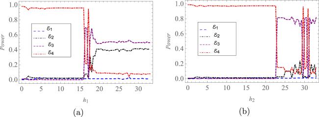
Figure 8. Energy flux versus (a) plasma beam radius h1 and (b) dielectric radius h2. |

Figure 9. Energy flux versus (a) plasma radius a and (b) angular frequency ω. |
To analyze the effect of increasing plasma frequency, the energy flux is displayed in terms of ωp/ω in figure 10(a), the range being taken as 0 < ωp/ω < 1.2. It is obvious from the figure that no transmission takes place after 0.94. As the plasma frequency equals the angular frequency, the reflected and transmitted powers become zero. The transmission remains zero and all the energy is reflected with the increase in ωp. This complies with the fact that the propagation of electromagnetic waves does not occur if the plasma frequency is greater than wave frequency ω. The plot of power with respect to ωb/ω, revealed in figure 10(b), shows that the increase in beam frequency ωb results in a gradual increase in the reflection of electromagnetic waves. The values vary between 0 < ωb/ω < 1.6.
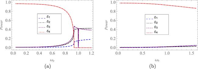
Figure 10. Energy flux versus (a) plasma frequency ωp and (b) beam frequency ωb. |
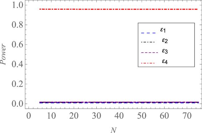
The conserved power also suggests that the truncated solution is convergent. The accuracy is checked up to six decimal places. It is observed that the impact of the truncation becomes infinitesimal when N ≥ 50. This is obvious from table 1 as well as from figure 11. Therefore, the given system of infinite equations can easily be treated as finite.
Figure 11. Power flux plotted against truncated terms N. |
Table 1. Energy conservation versus number of terms N. |
| Terms (N) | ${{ \mathcal E }}_{1}$ | ${{ \mathcal E }}_{2}$ | ${{ \mathcal E }}_{3}$ | ${{ \mathcal E }}_{4}$ | ${{ \mathcal E }}_{t}$ |
|---|---|---|---|---|---|
| 10 | 0.010 434 | 0.015 087 | 0.016 378 | 0.958 101 | 1 |
| 20 | 0.010 596 | 0.015 090 | 0.016 345 | 0.957 969 | 1 |
| 30 | 0.010 493 | 0.015 347 | 0.016 324 | 0.957 836 | 1 |
| 40 | 0.010 473 | 0.015 508 | 0.016 304 | 0.957 715 | 1 |
| 50 | 0.010 570 | 0.015 505 | 0.016 294 | 0.957 631 | 1 |
| 60 | 0.010 538 | 0.015 593 | 0.016 285 | 0.957 584 | 1 |
| 70 | 0.010 552 | 0.015 655 | 0.016 275 | 0.957 518 | 1 |
Cut-on modes in regard to the plasma and vacuum radius a are computed and presented in table 2. The regions R1, R2, R3 and R4 are already mentioned in section 2 . The increase in beam radius h1 and angular frequency ω does not affect the number of cut-on modes, i.e. there exists only one cut-on mode in each region.
Table 2. Cut-on modes versus duct radius a. |
| Height (a) | R1 | R2 | R3 | R4 |
|---|---|---|---|---|
| 3.33333 | 1 | 1 | 1 | 1 |
| 5.16667 | 1 | 1 | 1 | 2 |
| 5.75000 | 1 | 1 | 2 | 2 |
| 8.75000 | 1 | 1 | 2 | 3 |
| 8.91667 | 1 | 1 | 3 | 3 |
| 12.25000 | 1 | 1 | 3 | 4 |
| 15.75000 | 1 | 1 | 3 | 5 |
6. Summary and conclusion
A detailed analysis of the propagation of electromagnetic waves, within a metallic conducting cylindrical waveguide having plasma beam encompassed by cold plasma, has been carried out. Plasma conductivity has a substantial influence on the propagation of electromagnetic waves in the proposed design. This structure has its utility as a high-power microwave source and in cavity resonators.
The physical configuration includes a plasma beam embedded in cold collisionless plasma within an unbounded waveguide. The waveguide is composed of semi-bounded left and right duct regions z < 0 and z > 0, respectively, and has a perfectly conducting wall of radius a. The left section is configured as vacuum-dielectric-vacuum, bounded by metallic walls at r = h1, h2 and a, respectively. The corresponding boundary value problem was formed into an infinite system of linear algebraic equations.
The matching conditions were reconstructed in order to confirm the accuracy of the truncated solution. The real and imaginary parts of the electromagnetic fields were observed to match perfectly at the interface. The energy distribution within this waveguide was also explored. It was noted through computations and plots that the increase in duct radius h1 leads to an increase in transmission and an increase in dielectric radius h2 results in fluctuation in power. However, power seems to be transmitted completely through the beam and plasma as the duct radius a increases. The factor driving this phenomenon is the conductivity of plasma. It was also noted that as the angular frequency becomes larger than the plasma and beam frequencies, total transmission of the electromagnetic waves takes place within the waveguide. The increase in beam and plasma frequencies, with respect to the angular frequency, creates a negative impact on the transmission of electromagnetic waves. Cut-on modes were also calculated for all regions of this waveguide. The number of cut-on modes in the right duct and in the vacuum in the left duct region, where h2 < r < a, increased with the increase in the cold plasma radius a. Conversely, the increase in beam radius and angular frequency did not affect the number of cut-on modes in any region. The arrangement inside the right duct of this cylindrical waveguide is comparable to the design presented by Hong-Quan and Pu-Kun [21] in their paper. However, the numerical results and conclusions are different.
This investigation can be applied extensively to different plasma-filled structures, for example, in the form of a cylindrical waveguide in which the right duct can be treated as a chamber enclosed between vacuum-dielectric-vacuum setting in the left and right ducts. A cylindrical waveguide having a plasma beam wrapped around by cold unmagnetized plasma and a dielectric, but separated by conducting walls, can also be analyzed.