


1. Introduction
Path integral formalism is one of the most suitable tools in studying the thermal and dynamical properties of the quantum open systems [1–6]. Path integral formalism was proposed by Feynman [7–9], by which he showed that the matrix element of the canonical or evolution operator of a quantum system can be represented as a sum over histories of imaginary or real-time paths in configuration space. The general path integral formalism of a quantum system with linear dissipating in a bosonic environment was developed by Feynman and Vernon [10], which was later concretized to the well known Caldeira–Leggett model [1, 11, 12]. The corresponding Hamiltonian is usually written in a system-plus-environment form as
$\begin{eqnarray}\hat{H}={\hat{H}}_{{\rm{S}}}+{\hat{H}}_{{\rm{E}}}+{\hat{H}}_{\mathrm{SE}},\end{eqnarray}$
where ${\hat{H}}_{{\rm{S}}}$ is the system Hamiltonian, ${\hat{H}}_{{\rm{E}}}$ is the environment Hamiltonian, and ${\hat{H}}_{\mathrm{SE}}$ represents the system-environment coupling. For a single bath Caldeira–Leggett model, where the environment contains a single bath consisting of a set of bosons, the environment Hamiltonian is ${\hat{H}}_{{\rm{E}}}={\sum }_{k}{\omega }_{k}{\hat{b}}_{k}^{\dagger }{\hat{b}}_{k}$ with ${\hat{b}}_{k}^{\dagger }$ (${\hat{b}}_{k}$) being the annihilation (creation) operators of a mode k boson with frequency ωk. The coupling term is written as ${\hat{H}}_{\mathrm{SE}}=\hat{\sigma }{\sum }_{k}{V}_{k}({\hat{b}}_{k}^{\dagger }+{\hat{b}}_{k})$, where $\hat{\sigma }$ is a Hermite system operator and Vk is the coupling strength. The bath is characterized by the spectrum function $J(\omega )={\sum }_{k}{V}_{k}^{2}\delta (\omega -{\omega }_{k})$.Let us consider the imaginary-time path integral formalism of the partition function $Z={{\rm{Tre}}}^{-\beta \hat{H}}$ here. For a single bath model, we can find an eigenbasis ∣s⟩ of $\hat{\sigma }$ with s being the corresponding eigenvalue, as a complete set of the system. Let ∣n⟩ be the complete set of the bath, then the identity operator for the whole system is ${\sum }_{s,n}| {sn}\rangle \langle {sn}| $. Splitting β = (N + 1)δτ with N → ∞ , the partition function becomes (throughout this article we use ℏ = kB = 1)4 ) and the influence functional (5 ) is of no ambiguity.
$\begin{eqnarray}\begin{array}{rcl}Z & = & \mathrm{Tr}\,[{{\rm{e}}}^{-\delta \tau \hat{H}}\cdots {{\rm{e}}}^{-\delta \tau \hat{H}}]\\ & = & \displaystyle \sum _{{s}_{0},\ldots ,{s}_{N}}\displaystyle \sum _{{n}_{0},\ldots ,{n}_{N}}\langle {s}_{0}{n}_{0}| {{\rm{e}}}^{-\delta \tau \hat{H}}| {s}_{N}{n}_{N}\rangle \cdots \langle {s}_{1}{n}_{1}| {{\rm{e}}}^{-\delta \tau \hat{H}}| {s}_{0}{n}_{0}\rangle .\end{array}\end{eqnarray}$
After tracing over the bath degrees of freedom, Z can be written in the path integral formalism as [1, 2, 6, 13–15] $\begin{eqnarray}Z={Z}_{{\rm{E}}}\int { \mathcal D }[s(\tau )]K[s(\tau )]I[s(\tau )],\end{eqnarray}$
where ZE is the free bath partition function, and the notation $\int { \mathcal D }[s(\tau )]={\sum }_{{s}_{0},\ldots ,{s}_{N}}$ means the summation over all possible trajectories of s(τ) = {s0,…,sN}. The term K[s(τ)] is the bare system propagator $\begin{eqnarray}\begin{array}{rcl}K[s(\tau )] & = & \langle {s}_{0}| {{\rm{e}}}^{-\delta \tau {\hat{H}}_{{\rm{S}}}}| {s}_{N}\rangle \langle {s}_{N}| {{\rm{e}}}^{-\delta \tau {\hat{H}}_{{\rm{S}}}}| {s}_{N-1}\rangle \\ & & \cdots \langle {s}_{1}| {{\rm{e}}}^{-\delta \tau {\hat{H}}_{{\rm{S}}}}| {s}_{0}\rangle ,\end{array}\end{eqnarray}$
which is a (N + 1)-dimensional scalar-valued ‘tensor'. The term I[s(τ)] is referred to as the influence functional, and in the continuous limit is written as $\begin{eqnarray}I[s(\tau )]={{\rm{e}}}^{-{\int }_{0}^{\beta }{\rm{d}}\tau {\int }_{0}^{\beta }{\rm{d}}\tau ^{\prime} s(\tau ){\rm{\Delta }}(\tau ,\tau ^{\prime} )s(\tau ^{\prime} )}.\end{eqnarray}$
Here, ${\rm{\Delta }}(\tau ,\tau ^{\prime} )$ is the hybridization function ${\rm{\Delta }}(\tau ,\tau ^{\prime} )\,=\int {\rm{d}}\omega J(\omega ){D}_{\omega }(\tau ,\tau ^{\prime} )$, where ${D}_{\omega }(\tau ,\tau ^{\prime} )=-\langle {T}_{\tau }{\hat{b}}_{\omega }(\tau ){\hat{b}}_{\omega }^{\dagger }(\tau ^{\prime} ){\rangle }_{{\rm{E}}}$ (Tτ is the imaginary time-ordered operator) is the free bath Matsubara Green's function. Since s(τ) is just a scalar here, the influence functional is also a (N + 1)-dimensional tensor $I[s(\tau )]={I}_{{s}_{0},\ldots ,{s}_{N}}$. In this situation, the meaning of the bare system propagator (However, the situation becomes different when we can not use an eigenbasis of $\hat{\sigma }$ as a complete set of the system, i.e., when the system-bath coupling is non-diagonal. This can happen when the environment contains several baths. Suppose we have two baths, and they couple to the system via system operators ${\hat{\sigma }}_{1}$ and ${\hat{\sigma }}_{2}$. If ${\hat{\sigma }}_{1}$ and ${\hat{\sigma }}_{2}$ are not commutative for which $[{\hat{\sigma }}_{1},{\hat{\sigma }}_{2}]\ne 0$, then it is not possible to find a common eigenbasis for both of them. Compared to the diagonal system-bath coupling situation, which has been well studied in path integral formalism, the non-diagonal situation is much less studied. The non-diagonal path integral formalism has been employed in the hierarchical equations of motion (HEOM) method [16, 17] and the tensor-network based method [18], studying the quantum open system with non-additive environments. As an example, it has been shown that the non-commutative system-bath couplings can lead to population inversion of the two-level dipole [19].
In a non-diagonal situation, we can obtain the influence functional using an abstract method based on the Liouvillian superoperator [6, 20, 21] as5 ). In the HEOM framework, such a formalism is also obtained by this Liouvillian superoperator method [17]. We also note that the non-diagonal coupling terms of the system can be also handled by the coherent state representation in HEOM framework [22, 23]. Although we have successfully obtained the formula of the influence functional, the meaning of (6 ) is much less clear than (5 ). The value of (6 ) is not simply a scalar but a superoperator, and on what space do these $\hat{\sigma }(\tau )$ act and what order they are following needs some careful consideration [18, 20]. Additionally, in (6 ) the concept of trajectories also becomes ambiguous. It should be noted that by using the Dyson expansion method, we can also obtain a similar superoperator-valued influence functional formalism [24], but it works in perturbative expansion, not the path integral scenario.
$\begin{eqnarray}I[\hat{\sigma }(\tau )]={{\rm{e}}}^{-{\int }_{0}^{\beta }{\rm{d}}\tau ^{\prime} {\int }_{0}^{\beta }{\rm{d}}\tau ^{\prime\prime} \hat{\sigma }(\tau ^{\prime} ){\rm{\Delta }}(\tau ^{\prime} ,\tau ^{\prime\prime} )\hat{\sigma }(\tau ^{\prime\prime} )},\end{eqnarray}$
where we have just replaced the scalar trajectories s(τ) by the corresponding operator trajectories $\hat{\sigma }(\tau )$ in (In this article, instead of using the abstract Liouvillian method to derive (6 ), we give a concrete derivation based on the straightforward Trotter splitting as (2 ). Although such a derivation may look more cumbersome, it provides a clear picture to interpret the superoperator-valued influence functional (6 ).
2. Derivation
For ease of exposition, let us first consider the imaginary-time path integral formalism and assume that the bath only consists of a single boson mode. The extension to continuous spectrum bosons is straightforward. Then, the bath Hamiltonian writes ${\hat{H}}_{{\rm{E}}}=\omega {\hat{b}}^{\dagger }\hat{b}$, and the system-bath coupling term is ${\hat{H}}_{\mathrm{SE}}=\hat{\sigma }V({\hat{b}}^{\dagger }+\hat{b})$. Suppose the system and bath are in thermal equilibrium with the density matrix $\hat{\rho }={{\rm{e}}}^{-\beta \hat{H}}$, where β is the inverse temperature. The partition function is defined as $Z={\mathrm{Tre}}^{-\beta \hat{H}}$, and now we want to express Z in path integral formalism. Splitting β into β = (N + 1)δτ with N → ∞ yields $Z=\mathrm{Tr}[{{\rm{e}}}^{-\delta \tau \hat{H}}\cdots {{\rm{e}}}^{-\delta \tau \hat{H}}]$, and then employing the Trotter–Suzuki decomposition [25, 26] gives
$\begin{eqnarray}Z=\mathrm{Tr}[{{\rm{e}}}^{-\delta \tau {\hat{H}}_{{\rm{S}}}}{{\rm{e}}}^{-\delta \tau ({\hat{H}}_{{\rm{E}}}+{\hat{H}}_{\mathrm{SE}})}\cdots {{\rm{e}}}^{-\delta \tau {\hat{H}}_{{\rm{S}}}}{{\rm{e}}}^{-\delta \tau ({\hat{H}}_{{\rm{E}}}+{\hat{H}}_{\mathrm{SE}})}].\end{eqnarray}$
It is convenient to use the boson coherent state to eliminate the bath degrees of freedom. The boson coherent state [3, 27] is defined as the eigenstate of the annihilation operator for which $\hat{b}| \varphi \rangle =\varphi | \varphi \rangle $ and $\langle \varphi | {\hat{b}}^{\dagger }=\langle \varphi | \bar{\varphi }$, where $\varphi ,\bar{\varphi }$ are a complex number and its complex conjugate. With the aid of the coherent state, the identity operator for the bath can be expressed as7 ) gives11 ), and the expression of Z would reduce to3 ). Here, the hybridization function is ${\rm{\Delta }}(\tau ,\tau ^{\prime} )={V}^{2}D(\tau ,\tau ^{\prime} )$, where $D(\tau ,\tau ^{\prime} )=-\langle {T}_{\tau }\hat{b}(\tau ){\hat{b}}^{\dagger }(\tau ){\rangle }_{{\rm{E}}}$ is the free bath Matsubara Green's function. If the bath consists of a set of bosons with continuous spectrum, then we need to only replace the hybridization function by the one described by the bath spectrum function as ${\rm{\Delta }}(\tau ,\tau ^{\prime} )=\int {\rm{d}}\omega J(\omega ){D}_{\omega }(\tau ,\tau ^{\prime} )$.
$\begin{eqnarray}\int \displaystyle \frac{{\rm{d}}\bar{\varphi }{\rm{d}}\varphi }{2\pi {\rm{i}}}{{\rm{e}}}^{-\bar{\varphi }\varphi }|\varphi \rangle \langle \varphi |.\end{eqnarray}$
Accordingly, the trace over the bath can be written as $\begin{eqnarray}{\mathrm{Tr}}_{{\rm{E}}}[\cdots ]=\int \displaystyle \frac{{\rm{d}}\bar{\varphi }{\rm{d}}\varphi }{2\pi {\rm{i}}}{{\rm{e}}}^{-\bar{\varphi }\varphi }\langle \varphi | \cdots | \varphi \rangle .\end{eqnarray}$
Let ∣s⟩ denote a complete set of the system, which need not to be an eigenbasis of $\hat{\sigma }$, then the identity operator for the system is ∑s∣s⟩⟨s∣ and the trace over the system is ${\mathrm{Tr}}_{{S}}[\cdots ]={\sum }_{s}\cdots $. The full identity operator is then $\begin{eqnarray}\displaystyle \sum _{s}\int \displaystyle \frac{{\rm{d}}\bar{\varphi }{\rm{d}}\varphi }{2\pi {\rm{i}}}{{\rm{e}}}^{-\bar{\varphi }\varphi }| s\varphi \rangle \langle s\varphi | .\end{eqnarray}$
Inserting the corresponding identity operator between every two exponentials in ( $\begin{eqnarray}\begin{array}{l}Z=\displaystyle \sum _{{s}_{0},\ldots ,{s}_{N}}\displaystyle \sum _{{s}_{0}^{{\prime} },\ldots ,{s}_{N}^{{\prime} }}\displaystyle \int \left[\displaystyle \prod _{\alpha =0}^{N}\displaystyle \frac{{\rm{d}}{\bar{\varphi }}_{\alpha }{\rm{d}}{\varphi }_{\alpha }}{2\pi {\rm{i}}}{{\rm{e}}}^{-{\bar{\varphi }}_{\alpha }{\varphi }_{\alpha }}\right]\\ \,\times \langle {s}_{0}| {{\rm{e}}}^{-\delta \tau {\hat{H}}_{{\rm{S}}}}| {s}_{N}^{{\prime} }\rangle \langle {s}_{N}^{{\prime} }| {{\rm{e}}}^{a{\bar{\varphi }}_{0}{\varphi }_{N}-\delta \tau V\hat{\sigma }({\bar{\varphi }}_{0}+{\varphi }_{N})}| {s}_{N}\rangle \\ \,\times \cdots \langle {s}_{1}| {{\rm{e}}}^{-\delta \tau {\hat{H}}_{{\rm{S}}}}| {s}_{0}^{{\prime} }\rangle \langle {s}_{0}^{{\prime} }| {{\rm{e}}}^{a{\bar{\varphi }}_{1}{\varphi }_{0}-\delta \tau V\hat{\sigma }({\bar{\varphi }}_{1}+{\varphi }_{0})}| {s}_{0}\rangle ,\end{array}\end{eqnarray}$
where a = 1 − δτω = e−δτω. Here, we have used the fact that $\langle {\varphi }_{1}| {\varphi }_{0}\rangle ={{\rm{e}}}^{{\bar{\varphi }}_{1}{\varphi }_{0}}$ and $\begin{eqnarray}\begin{array}{l}\langle {s}_{1}{\varphi }_{1}| {{\rm{e}}}^{-\delta \tau {\hat{H}}_{{\rm{S}}}}{{\rm{e}}}^{-\delta \tau ({\hat{H}}_{{\rm{E}}}+{\hat{H}}_{\mathrm{SE}})}| {s}_{0}{\varphi }_{0}\rangle \\ =\displaystyle \sum _{{s}_{0}^{{\prime} }}\langle {s}_{1}| {{\rm{e}}}^{-\delta \tau {\hat{H}}_{{\rm{S}}}}| {s}_{0}^{{\prime} }\rangle \langle {s}_{0}^{{\prime} }| {{\rm{e}}}^{a{\bar{\varphi }}_{1}{\varphi }_{0}-\delta \tau V\hat{\sigma }({\bar{\varphi }}_{1}+{\varphi }_{0})}| {s}_{0}\rangle .\end{array}\end{eqnarray}$
If ∣s⟩ is an eigenbasis of $\hat{\sigma }$, then we can get rid of variables with prime $s^{\prime} $ in ( $\begin{eqnarray}\begin{array}{rcl}Z & = & \displaystyle \sum _{{s}_{0},\ldots ,{s}_{N}}\displaystyle \int \left[\displaystyle \prod _{\alpha =0}^{N}\displaystyle \frac{{\rm{d}}{\bar{\varphi }}_{\alpha }{\rm{d}}{\varphi }_{\alpha }}{2\pi {\rm{i}}}{{\rm{e}}}^{-{\bar{\varphi }}_{\alpha }{\varphi }_{\alpha }}\right]\\ & & \times \ \langle {s}_{N}| {{\rm{e}}}^{-\delta \tau {\hat{H}}_{{\rm{S}}}}| {s}_{N-1}\rangle \cdots \langle {s}_{1}| {{\rm{e}}}^{-\delta \tau {\hat{H}}_{{\rm{S}}}}| {s}_{0}\rangle \\ & & \times {{\rm{e}}}^{a{\bar{\varphi }}_{0}{\varphi }_{N}-\delta \tau {{Vs}}_{N}({\bar{\varphi }}_{0}+{s}_{N}{\varphi }_{N})}\cdots {{\rm{e}}}^{a{\bar{\varphi }}_{1}{\varphi }_{0}-\delta \tau {{Vs}}_{0}({\bar{\varphi }}_{1}+{s}_{0}{\varphi }_{0})}.\end{array}\end{eqnarray}$
The variables ${\bar{\varphi }}_{k},{\varphi }_{k}$ can be integrated out via Gaussian integral and we shall obtain the standard path integral formula (However, if ∣s⟩ is not an eigenbasis of $\hat{\sigma }$, then we can not simply get rid of $s^{\prime} $ in (11 ). We have the system operator $\hat{\sigma }$ in the exponential and thus the Gaussian integral over $\bar{\varphi },\varphi $ can not be applied. To resolve this issue, we first diagonalize the operator $\hat{\sigma }$ by some unitary transformation as $\hat{\sigma }={\hat{S}}^{\dagger }\hat{{\rm{\Sigma }}}\hat{S}$. Let ∣σ⟩ be an eigenbasis of $\hat{{\rm{\Sigma }}}$ with eigenvalue σ, then we can write11 ) becomes13 ), therefore integrating out $\bar{\varphi },\varphi $ yields
$\begin{eqnarray}\langle {s}_{0}^{{\prime} }| {{\rm{e}}}^{-\delta \tau V\hat{\sigma }({\bar{\varphi }}_{1}+{\varphi }_{0})}| {s}_{0}\rangle =\displaystyle \sum _{\sigma }\langle {s}_{0}^{{\prime} }| {\hat{S}}^{\dagger }| \sigma \rangle {{\rm{e}}}^{-\delta \tau V\sigma ({\bar{\varphi }}_{1}+{\varphi }_{0})}\langle \sigma | \hat{S}| {s}_{0}\rangle ,\end{eqnarray}$
and ( $\begin{eqnarray}\begin{array}{rcl}Z & = & \displaystyle \sum _{{s}_{0},\ldots ,{s}_{N}}\displaystyle \sum _{{s}_{0}^{{\prime} },\ldots ,{s}_{N}^{{\prime} }}\displaystyle \sum _{{\sigma }_{0},\ldots ,{\sigma }_{N}}\displaystyle \int \left[\displaystyle \prod _{\alpha =0}^{N}\displaystyle \frac{{\rm{d}}{\bar{\varphi }}_{\alpha }{\rm{d}}{\varphi }_{\alpha }}{2\pi {\rm{i}}}{{\rm{e}}}^{-{\bar{\varphi }}_{\alpha }{\varphi }_{\alpha }}\right]\\ & & \times \langle {s}_{0}| {{\rm{e}}}^{-\delta \tau {\hat{H}}_{{\rm{S}}}}| {s}_{N}^{{\prime} }\rangle \langle {s}_{N}^{{\prime} }| {\hat{S}}^{\dagger }| {\sigma }_{N}\rangle \langle {\sigma }_{N}| \hat{S}| {s}_{N}\rangle \\ & & \times \cdots \langle {s}_{1}| {{\rm{e}}}^{-\delta \tau {\hat{H}}_{{\rm{S}}}}| {s}_{0}^{{\prime} }\rangle \langle {s}_{0}^{{\prime} }| {\hat{S}}^{\dagger }| {\sigma }_{0}\rangle \langle {\sigma }_{0}| \hat{S}| {s}_{0}\rangle \\ & & \times {{\rm{e}}}^{a{\bar{\varphi }}_{0}{\varphi }_{N}-\delta \tau V{\sigma }_{N}({\bar{\varphi }}_{0}+{\varphi }_{N})}\cdots {{\rm{e}}}^{a{\bar{\varphi }}_{1}{\varphi }_{0}-\delta \tau V{\sigma }_{0}({\bar{\varphi }}_{1}+{\varphi }_{0})}.\end{array}\end{eqnarray}$
It can be seen that in the above expression, all quantities are reduced to ordinary scalars, therefore the Gaussian integral over $\bar{\varphi },\varphi $ is applicable again. The terms involving $\bar{\varphi },\varphi $ in the above expression have the same form as that of ( $\begin{eqnarray}\begin{array}{rcl}Z & = & \displaystyle \sum _{{s}_{0},\ldots ,{s}_{N}}\displaystyle \sum _{{s}_{0}^{{\prime} },\ldots ,{s}_{N}^{{\prime} }}\displaystyle \sum _{{\sigma }_{0},\ldots ,{\sigma }_{N}}{{\rm{e}}}^{-{\displaystyle \int }_{0}^{\beta }{\rm{d}}\tau ^{\prime} {\displaystyle \int }_{0}^{\beta }{\rm{d}}\tau ^{\prime\prime} \sigma (\tau ^{\prime} ){\rm{\Delta }}(\tau ^{\prime} ,\tau ^{\prime\prime} )\sigma (\tau ^{\prime\prime} )}\\ & & \times \langle {s}_{0}| {{\rm{e}}}^{-\delta \tau {\hat{H}}_{{\rm{S}}}}| {s}_{N}^{{\prime} }\rangle \langle {s}_{N}^{{\prime} }| {\hat{S}}^{\dagger }| {\sigma }_{N}\rangle \langle {\sigma }_{N}| \hat{S}| {s}_{N}\rangle \\ & & \times \cdots \langle {s}_{1}| {{\rm{e}}}^{-\delta \tau {\hat{H}}_{{\rm{S}}}}| {s}_{0}^{{\prime} }\rangle \langle {s}_{0}^{{\prime} }| {\hat{S}}^{\dagger }| {\sigma }_{0}\rangle \langle {\sigma }_{0}| \hat{S}| {s}_{0}\rangle .\end{array}\end{eqnarray}$
This expression is similar to the standard diagonal path integral formalism (3 ), except that K is modified by including the auxiliary state ∣σ⟩ and the transformation operator $\hat{S},{\hat{S}}^{\dagger }$. This is the desired formula for the non-diagonal system-bath coupling situation, and now we try to write it in a more compact form. The terms ∑s∣s⟩⟨s∣ and ${\sum }_{s^{\prime} }| s^{\prime} \rangle \langle s^{\prime} | $ in the above expression, unlike ∑σ∣σ⟩⟨σ∣, are not correlated with other terms, therefore we can write them back as the system identity operator. By doing so, the above expression can be written in an operator form as17 ) symbolically as17 ) symbolically in a similar form of standard path integral (3 ) as6 ), and its meaning is clearly shown in (17 ). This expression may also be interpreted in the way that the operator $\hat{\sigma }(t)$ acts on the system history Hilbert space as described in [18, 20].
$\begin{eqnarray}\begin{array}{l}Z={Z}_{{\rm{E}}}\displaystyle \int { \mathcal D }[\sigma (\tau )]{{\rm{e}}}^{-{\displaystyle \int }_{0}^{\beta }{\rm{d}}\tau ^{\prime} {\displaystyle \int }_{0}^{\beta }{\rm{d}}\tau ^{\prime\prime} \sigma (\tau ^{\prime} ){\rm{\Delta }}(\tau ^{\prime} ,\tau ^{\prime\prime} )\sigma (\tau ^{\prime\prime} )}{\mathrm{Tr}}_{{\rm{S}}}\\ \,\times \ [{{\rm{e}}}^{-\delta \tau {\hat{H}}_{{\rm{S}}}}{\hat{S}}^{\dagger }| {\sigma }_{N}\rangle \langle {\sigma }_{N}| \hat{S}\cdots {{\rm{e}}}^{-\delta \tau {\hat{H}}_{{\rm{S}}}}{\hat{S}}^{\dagger }| {\sigma }_{0}\rangle \langle {\sigma }_{0}| \hat{S}].\end{array}\end{eqnarray}$
Since ${{\rm{e}}}^{\hat{\sigma }}={\hat{S}}^{\dagger }{{\rm{e}}}^{\hat{{\rm{\Sigma }}}}\hat{S}$, we symbolically denote ${\sum }_{\sigma }{\hat{S}}^{\dagger }| \sigma \rangle {{\rm{e}}}^{\sigma }\langle \sigma | \hat{S}$ as ${{\rm{e}}}^{\hat{\sigma }}$. Then the terms in the trace may be viewed as a product of sequence ${{\rm{e}}}^{-\delta \tau {\hat{H}}_{{\rm{S}}}}{{\rm{e}}}^{\hat{\sigma }}\cdots {{\rm{e}}}^{-\delta \tau {\hat{H}}_{{\rm{S}}}}{{\rm{e}}}^{\hat{\sigma }}$ where ${{\rm{e}}}^{-\delta \tau {\hat{H}}_{{\rm{S}}}}$ and ${{\rm{e}}}^{\hat{\sigma }}$ are alternately placed. It should be emphasized that due to the existence of the exponential term ${{\rm{e}}}^{-{\int }_{0}^{\beta }{\rm{d}}\tau ^{\prime} {\int }_{0}^{\beta }{\rm{d}}\tau ^{\prime\prime} \sigma (\tau ^{\prime} ){\rm{\Delta }}(\tau ^{\prime} ,\tau ^{\prime\prime} )\sigma (\tau ^{\prime\prime} )}$, all ${{\rm{e}}}^{\hat{\sigma }}$ terms are correlated to each other. Now, we denote the sequence ${{\rm{e}}}^{-\delta \tau {\hat{H}}_{{\rm{S}}}}\cdots {{\rm{e}}}^{-\delta \tau {\hat{H}}_{{\rm{S}}}}$ as $\begin{eqnarray}\begin{array}{l}K[{\hat{H}}_{{\rm{S}}}(\tau )]={T}_{\tau }{{\rm{e}}}^{-{\displaystyle \int }_{0}^{\beta }{\rm{d}}\tau {\hat{H}}_{{\rm{S}}}(\tau )}={{\rm{e}}}^{-\delta \tau {\hat{H}}_{{\rm{S}}}}\bigsqcup {{\rm{e}}}^{-\delta \tau {\hat{H}}_{{\rm{S}}}}\bigsqcup \cdots \bigsqcup {{\rm{e}}}^{-\delta \tau {\hat{H}}_{{\rm{S}}}},\end{array}\end{eqnarray}$
where Tτ is an imaginary time-ordered operator which means that in the sequence the index increases from right to left. The symbol ⨆ indicates that at this time the terms ${{\rm{e}}}^{-\delta \tau {\hat{H}}_{{\rm{S}}}}$ in the sequence are not connected, i.e., the multiplication between them is not applied yet. We denote the term $K[{\hat{H}}_{{\rm{S}}}(\tau )]$ as generalized system propagator. Following the same spirit, we write the rest terms in ( $\begin{eqnarray}\begin{array}{rcl}I[\hat{\sigma }(\tau )] & = & {{\rm{e}}}^{-{\displaystyle \int }_{0}^{\beta }{\rm{d}}\tau ^{\prime} {\displaystyle \int }_{0}^{\beta }{\rm{d}}\tau ^{\prime\prime} \sigma (\tau ^{\prime} ){\rm{\Delta }}(\tau ^{\prime} ,\tau ^{\prime\prime} )\sigma (\tau ^{\prime\prime} )}\\ & & \times \ [{\hat{S}}^{\dagger }| \sigma \rangle \langle \sigma | \hat{S}\bigsqcup {\hat{S}}^{\dagger }| \sigma \rangle \langle \sigma | \hat{S}\bigsqcup {\hat{S}}^{\dagger }| \sigma \rangle \langle \sigma | \hat{S}\bigsqcup \cdots \bigsqcup {\hat{S}}^{\dagger }| \sigma \rangle \langle \sigma | \hat{S}]\\ & = & {{\rm{e}}}^{-{\displaystyle \int }_{0}^{\beta }{\rm{d}}\tau ^{\prime} {\displaystyle \int }_{0}^{\beta }{\rm{d}}\tau ^{\prime\prime} \hat{\sigma }(\tau ^{\prime} ){\rm{\Delta }}(\tau ^{\prime} ,\tau ^{\prime\prime} )\hat{\sigma }(\tau ^{\prime\prime} )}.\end{array}\end{eqnarray}$
We denote this expression as generalized influence functional, which is also viewed as a sequence where multiplication is not applied yet. Then, we write the partition function ( $\begin{eqnarray}Z={Z}_{{\rm{E}}}{{\rm{Tr}}}_{{\rm{S}}}\int { \mathcal D }[\sigma (\tau )]K[{\hat{H}}_{{\rm{S}}}(\tau )]\wedge I[\hat{\sigma }(\tau )].\end{eqnarray}$
Here, the symbol ∧ means that sequences $K[{\hat{H}}_{{\rm{S}}}(\tau )]$ and $I[\hat{\sigma }(t)]$ are alternately placed, and then the multiplication between all terms is applied. The corresponding procedure is illustrated in figure 1. In this manner, we have obtained the desired superoperator-valued influence functional expression as (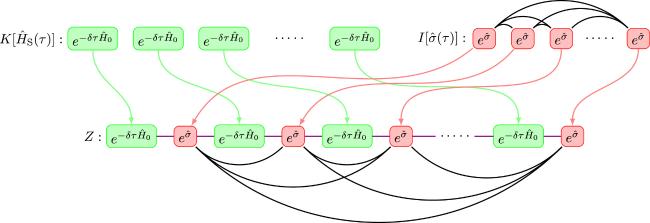
Figure 1. Illustration for expression ( |
Now, let us consider the situation where multiple baths are present. For simplicity, we consider a two baths situation first, where the Hamiltonian is written as20 ) as19 ) for the first and second bath, respectively, that25 ).
$\begin{eqnarray}\hat{H}={\hat{H}}_{{\rm{S}}}+{\hat{H}}_{{\rm{E}}}^{(1)}+{\hat{H}}_{{\rm{E}}}^{(2)}+{\hat{H}}_{\mathrm{SE}}^{(1)}+{\hat{H}}_{\mathrm{SE}}^{(2)},\end{eqnarray}$
where ${\hat{H}}_{{\rm{E}}}^{(1)}={\omega }_{1}{\hat{b}}_{1}^{\dagger }{\hat{b}}_{1},{\hat{H}}_{{\rm{E}}}^{(2)}={\omega }_{2}{\hat{b}}_{2}^{\dagger }{\hat{b}}_{2}$ are the bath Hamiltonian for the first and second bath, respectively. The system-bath couplings are given by ${\hat{H}}_{\mathrm{SE}}^{(1)}={V}_{1}{\hat{\sigma }}_{1}({\hat{b}}_{1}^{\dagger }+{\hat{b}}_{1})$ and ${\hat{H}}_{\mathrm{SE}}^{(1)}={V}_{2}{\hat{\sigma }}_{2}({\hat{b}}_{2}^{\dagger }+{\hat{b}}_{2})$. The Trotter–Suzuki decomposition yields $\begin{eqnarray}\begin{array}{l}Z=\mathrm{Tr}\left[{{\rm{e}}}^{-\delta \tau {\hat{H}}_{{\rm{S}}}}{{\rm{e}}}^{-\delta \tau ({\hat{H}}_{{\rm{E}}}^{(1)}+{\hat{H}}_{\mathrm{SE}}^{(1)})}{{\rm{e}}}^{-\delta \tau ({\hat{H}}_{{\rm{E}}}^{(2)}+{\hat{H}}_{\mathrm{SE}}^{(2)})}\right.\\ \,\times \left.\cdots {{\rm{e}}}^{-\delta \tau {\hat{H}}_{{\rm{S}}}}{{\rm{e}}}^{-\delta \tau ({\hat{H}}_{{\rm{E}}}^{(1)}+{\hat{H}}_{\mathrm{SE}}^{(1)})}{{\rm{e}}}^{-\delta \tau ({\hat{H}}_{{\rm{E}}}^{(2)}+{\hat{H}}_{\mathrm{SE}}^{(2)})}\right].\end{array}\end{eqnarray}$
Inserting the identity operator between every two exponentials gives $\begin{eqnarray}\begin{array}{l}Z=\displaystyle \sum _{{s}_{0},\ldots ,{s}_{N}}\displaystyle \sum _{{s}_{0}^{{\prime} },\ldots ,{s}_{N}^{{\prime} }}\displaystyle \sum _{{s}_{0}^{{\prime\prime} },\ldots ,{s}_{N}^{{\prime\prime} }}\displaystyle \int \left[\displaystyle \prod _{\alpha =0}^{N}\displaystyle \frac{{\rm{d}}{\bar{\varphi }}_{\alpha }^{(1)}{\rm{d}}{\varphi }_{\alpha }^{(1)}}{2\pi {\rm{i}}}{{\rm{e}}}^{-{\bar{\varphi }}_{\alpha }^{(1)}{\varphi }_{\alpha }^{(1)}}\right]\\ \,\displaystyle \times \int \left[\displaystyle \prod _{\alpha =0}^{N}\displaystyle \frac{{\rm{d}}{\bar{\varphi }}_{\alpha }^{(2)}{\rm{d}}{\varphi }_{\alpha }^{(2)}}{2\pi {\rm{i}}}{{\rm{e}}}^{-{\bar{\varphi }}_{\alpha }^{(2)}{\varphi }_{\alpha }^{(2)}}\right]\\ \,\times \langle {s}_{0}| {{\rm{e}}}^{-\delta \tau {\hat{H}}_{{\rm{S}}}}| {s}_{N}^{{\prime} }\rangle \langle {s}_{N}^{{\prime} }| {{\rm{e}}}^{a{\varphi }_{0}^{(1)}{\varphi }_{N}^{(1)}-\delta \tau V{\hat{\sigma }}_{1}({\varphi }_{0}^{(1)}+{\varphi }_{N}^{(1)})}| {s}_{N}^{{\prime\prime} }\rangle \\ \,\times \langle {s}_{N}^{{\prime\prime} }| {{\rm{e}}}^{a{\varphi }_{0}^{(2)}{\varphi }_{N}^{(2)}-\delta \tau V{\hat{\sigma }}_{2}({\varphi }_{0}^{(2)}+{\varphi }_{N}^{(2)})}| {s}_{N}\rangle \\ \,\times \cdots \\ \,\times \langle {s}_{1}| {{\rm{e}}}^{-\delta \tau {\hat{H}}_{{\rm{S}}}}| {s}_{0}^{{\prime} }\rangle \langle {s}_{0}^{{\prime} }| {{\rm{e}}}^{a{\varphi }_{1}^{(1)}{\varphi }_{0}^{(1)}-\delta \tau V{\hat{\sigma }}_{1}({\varphi }_{1}^{(1)}+{\varphi }_{0}^{(1)})}| {s}_{0}^{{\prime\prime} }\rangle \\ \,\times \langle {s}_{0}^{{\prime\prime} }| {{\rm{e}}}^{a{\varphi }_{1}^{(2)}{\varphi }_{1}^{(2)}-\delta \tau V{\hat{\sigma }}_{2}({\varphi }_{1}^{(2)}+{\varphi }_{0}^{(2)})}| {s}_{0}\rangle .\end{array}\end{eqnarray}$
Diagonalize ${\hat{\sigma }}_{1},{\hat{\sigma }}_{2}$ as ${\hat{\sigma }}_{1}={\hat{S}}_{1}^{\dagger }{\hat{{\rm{\Sigma }}}}_{1}{\hat{S}}_{1},{\hat{\sigma }}_{2}={\hat{S}}_{2}^{\dagger }{\hat{{\rm{\Sigma }}}}_{2}{\hat{S}}_{2}$ with eigenvalues σ(1),σ(2) and integrate out ${\bar{\varphi }}^{(1)},{\varphi }^{(1)}$ and ${\bar{\varphi }}^{(2)},{\varphi }^{(2)}$, we should have $\begin{eqnarray}\begin{array}{l}Z=\displaystyle \sum _{{\sigma }_{0}^{(0)},\ldots ,{\sigma }_{N}^{(1)}}\displaystyle \sum _{{\sigma }_{0}^{(2)},\ldots ,{\sigma }_{N}^{(2)}}{{\rm{e}}}^{-{\displaystyle \int }_{0}^{\beta }{\rm{d}}\tau ^{\prime} {\displaystyle \int }_{0}^{\beta }{\rm{d}}\tau ^{\prime\prime} {\sigma }^{(1)}(\tau ^{\prime} ){{\rm{\Delta }}}^{(1)}(\tau ^{\prime} ,\tau ^{\prime\prime} ){\sigma }^{(1)}(\tau ^{\prime\prime} )}\\ \,\times {{\rm{e}}}^{-{\displaystyle \int }_{0}^{\beta }{\rm{d}}\tau ^{\prime} {\displaystyle \int }_{0}^{\beta }{\rm{d}}\tau ^{\prime\prime} {\sigma }^{(2)}(\tau ^{\prime} ){{\rm{\Delta }}}^{(2)}(\tau ^{\prime} ,\tau ^{\prime\prime} ){\sigma }^{(2)}(\tau ^{\prime\prime} )}\\ \,\times \displaystyle \sum _{{s}_{0},\ldots ,{s}_{N}}\displaystyle \sum _{{s}_{0}^{{\prime} },\ldots ,{s}_{N}^{{\prime} }}\displaystyle \sum _{{s}_{0}^{{\prime\prime} },\ldots ,{s}_{N}^{{\prime\prime} }}\langle {s}_{0}| {{\rm{e}}}^{-\delta \tau {\hat{H}}_{{\rm{S}}}}| {s}_{N}^{{\prime} }\rangle \langle {s}_{N}^{{\prime} }| {\hat{S}}_{1}^{\dagger }| {\sigma }_{N}^{(1)}\rangle \\ \,\times \langle {\sigma }_{N}^{(1)}| {\hat{S}}_{1}| {s}_{N}^{{\prime\prime} }\rangle \langle {s}_{N}^{{\prime\prime} }| {\hat{S}}_{2}^{\dagger }| {\sigma }_{N}^{(2)}\rangle \langle {\sigma }_{N}^{(2)}| {\hat{S}}_{2}| {s}_{N}\rangle \\ \,\times \cdots \langle {s}_{1}| {{\rm{e}}}^{-\delta \tau {\hat{H}}_{{\rm{S}}}}| {s}_{0}^{{\prime} }\rangle \langle {s}_{0}^{{\prime} }| {\hat{S}}_{1}^{\dagger }| {\sigma }_{0}^{(1)}\rangle \\ \,\times \langle {\sigma }_{0}^{(1)}| {\hat{S}}_{1}| {s}_{0}^{{\prime\prime} }\rangle \langle {s}_{0}^{{\prime\prime} }| {\hat{S}}_{2}^{\dagger }| {\sigma }_{0}^{(2)}\rangle \langle {\sigma }_{0}^{(2)}| {\hat{S}}_{2}| {s}_{0}\rangle ,\end{array}\end{eqnarray}$
where Δ(1) and Δ(2) are hybridization functions for the first and second bath, respectively. Following the same procedure shown before, this expression can be written in the generalized influence functional in a similar form to ( $\begin{eqnarray}Z={Z}_{{\rm{E}}}{\mathrm{Tr}}_{{\rm{S}}}\int { \mathcal D }[\sigma (\tau )]K[{\hat{H}}_{{\rm{S}}}(\tau )]\wedge {I}_{1}[{\hat{\sigma }}_{1}(\tau )]\wedge {I}_{2}[{\hat{\sigma }}_{2}(\tau )],\end{eqnarray}$
where I1 and I2 are generalized influence functionals in form of ( $\begin{eqnarray}\begin{array}{l}{I}_{1}[{\hat{\sigma }}_{1}(\tau )]\,=\,{{\rm{e}}}^{-{\displaystyle \int }_{0}^{\beta }{\rm{d}}\tau ^{\prime} {\displaystyle \int }_{0}^{\beta }{\rm{d}}\tau ^{\prime\prime} {\hat{\sigma }}_{1}(\tau ^{\prime} ){{\rm{\Delta }}}^{(1)}(\tau ^{\prime} ,\tau ^{\prime\prime} ){\hat{\sigma }}_{1}(\tau ^{\prime\prime} )},\\ {I}_{2}[{\hat{\sigma }}_{2}(\tau )]\,=\,{{\rm{e}}}^{-{\displaystyle \int }_{0}^{\beta }{\rm{d}}\tau ^{\prime} {\displaystyle \int }_{0}^{\beta }{\rm{d}}\tau ^{\prime\prime} {\hat{\sigma }}_{2}(\tau ^{\prime} ){{\rm{\Delta }}}^{(2)}(\tau ^{\prime} ,\tau ^{\prime\prime} ){\hat{\sigma }}_{2}(\tau ^{\prime\prime} )}.\end{array}\end{eqnarray}$
Figure 2 gives an illustration of (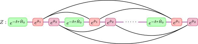
Figure 2. Illustration for the expression ( |
Similarly, if there are m baths, then the Hamiltonian can be written as29 ) means that the terms of the generalized system propagator and generalized influence functionals for all baths are alternately placed and then multiplied.
$\begin{eqnarray}\hat{H}={\hat{H}}_{{\rm{S}}}+\displaystyle \sum _{\alpha =1}^{m}[{\hat{H}}_{{\rm{E}}}^{(\alpha )}+{\hat{H}}_{\mathrm{SE}}^{(\alpha )}],\end{eqnarray}$
where ${\hat{H}}_{{\rm{E}}}^{(\alpha )}={\omega }_{\alpha }{\hat{b}}_{\alpha }^{\dagger }{\hat{b}}_{\alpha },{\hat{H}}_{\mathrm{SE}}^{\alpha }={V}_{\alpha }{\hat{\sigma }}_{\alpha }({\hat{b}}_{\alpha }^{\dagger }+{\hat{b}}_{\alpha })$. The Trotter–Suzuki decomposition yields $\begin{eqnarray}\begin{array}{rcl}Z & = & \mathrm{Tr}\left[{{\rm{e}}}^{-\delta \tau {\hat{H}}_{{\rm{S}}}}{{\rm{e}}}^{-\delta \tau ({\hat{H}}_{{\rm{E}}}^{(1)}+{\hat{H}}_{\mathrm{SE}}^{(1)})}\cdots {{\rm{e}}}^{-\delta \tau ({\hat{H}}_{{\rm{E}}}^{(m)}+{\hat{H}}_{\mathrm{SE}}^{(m)})}\right.\\ & & \times \left.\cdots {{\rm{e}}}^{-\delta \tau {\hat{H}}_{{\rm{S}}}}{{\rm{e}}}^{-\delta \tau ({\hat{H}}_{{\rm{E}}}^{(1)}+{\hat{H}}_{\mathrm{SE}}^{(1)})}\cdots {{\rm{e}}}^{-\delta \tau ({\hat{H}}_{{\rm{E}}}^{(m)}+{\hat{H}}_{\mathrm{SE}}^{(m)})}\right].\end{array}\end{eqnarray}$
Following the same procedure, we can obtain the generalized path integral formalism as $\begin{eqnarray}\begin{array}{rcl}Z & = & {\mathrm{Tr}}_{{\rm{S}}}\displaystyle \int { \mathcal D }[{\sigma }_{1}(\tau )]\cdots \displaystyle \int { \mathcal D }[{\sigma }_{m}(\tau )]\\ & & \times K[{\hat{H}}_{{\rm{S}}}(\tau )]\wedge {I}_{1}[{\hat{\sigma }}_{1}(\tau )]\wedge \cdots \wedge {I}_{m}[{\hat{\sigma }}_{m}(\tau )].\end{array}\end{eqnarray}$
where Δα is the hybridization function of αth bath $\begin{eqnarray}{I}_{\alpha }[{\hat{\sigma }}_{\alpha }(\tau )]={{\rm{e}}}^{-{\int }_{0}^{\beta }{\rm{d}}\tau ^{\prime} {\int }_{0}^{\beta }{\hat{\sigma }}_{\alpha }(\tau ^{\prime} ){{\rm{\Delta }}}_{\alpha }(\tau ^{\prime} ,\tau ^{\prime\prime} ){\hat{\sigma }}_{\alpha }(\tau ^{\prime\prime} )}.\end{eqnarray}$
The expression (3. Real-time dynamics
Now let us consider the real-time path integral formalism. For ease of exposition, we still assume a single bath with a single bosonic mode. Suppose at the initial time t = 0, the total density matrix is separated into the system and bath for which $\hat{\rho }={\hat{\rho }}_{{\rm{S}}}(0){\hat{\rho }}_{{\rm{E}}}$, where ${\hat{\rho }}_{{\rm{S}}}(0)$ is the initial system density matrix and the bath is in thermal equilibrium that ${\hat{\rho }}_{{\rm{E}}}={{\rm{e}}}^{-\beta {\hat{H}}_{{\rm{E}}}}$. According to the Von Neumann equation, the density matrix at time t = tf is $\hat{\rho }(t)={{\rm{e}}}^{-{\rm{i}}\hat{H}{t}_{f}}\hat{\rho }(0){{\rm{e}}}^{{\rm{i}}\hat{H}{t}_{f}}$.
It would be convenient to use Keldysh contour [15, 28–31] to describe the dynamics of the system. The contour starts from time zero and then goes to time tf, this part corresponds to forward evolution and thus we call it the forward branch. After arriving time tf, the contour returns to time zero, this part corresponds to the backward evolution and we call it the backward branch.
Let tf = (N + 1)δt with N → ∞, the Trotter–Suzuki decomposition gives
$\begin{eqnarray}\hat{\rho }({t}_{f})={\left[{{\rm{e}}}^{-{\rm{i}}{\hat{H}}_{{\rm{S}}}\delta t}{{\rm{e}}}^{-{\rm{i}}({\hat{H}}_{{\rm{E}}}+{\hat{H}}_{\mathrm{SE}})\delta t}\right]}^{N+1}\hat{\rho }(0){\left[{{\rm{e}}}^{{\rm{i}}({\hat{H}}_{{\rm{E}}}+{\hat{H}}_{\mathrm{SE}})\delta t}{{\rm{e}}}^{{\rm{i}}{\hat{H}}_{{\rm{S}}}\delta t}\right]}^{N+1}.\end{eqnarray}$
If we are working in the eigenbasis ∣s⟩ of $\hat{\sigma }$, then we shall obtain a path integral formula as $\begin{eqnarray}Z({t}_{f})=\mathrm{Tr}[\hat{\rho }({t}_{f})]=\int { \mathcal D }[s(t)]K[s(t)]I[s(t)],\end{eqnarray}$
where s(t) is a path on the Keldysh contour. Here, K[s(t)] is the free system propagator and I[s(t)] is the influence functional $\begin{eqnarray}I[s(t)]={{\rm{e}}}^{-{\int }_{{ \mathcal C }}{\rm{d}}t^{\prime} {\int }_{{ \mathcal C }}{\rm{d}}t^{\prime\prime} s(t^{\prime} ){\rm{\Delta }}(t^{\prime} ,t^{\prime\prime} )s(t^{\prime\prime} )},\end{eqnarray}$
and ${\rm{\Delta }}(t^{\prime} ,t^{\prime\prime} )={V}^{2}D(t^{\prime} ,t^{\prime\prime} )$ with $D(t^{\prime} ,t^{\prime\prime} )=\langle {T}_{{ \mathcal C }}\hat{b}(t^{\prime} ){\hat{b}}^{\dagger }(t^{\prime\prime} ){\rangle }_{{\rm{E}}}$ being the free contour-ordered Green's function of the bath. ${T}_{{ \mathcal C }}$ is the contour-ordered operator, and dt = ± δt on the forward (backward) branch.If we are not working in the eigenbasis of $\hat{\sigma }$, then employing the basic idea described in the previous section, we should obtain the partition function as29 ), if multiple baths are present, the partition function can be then written as
$\begin{eqnarray}\begin{array}{rcl}Z({t}_{f}) & = & \displaystyle \int { \mathcal D }[\hat{\sigma }(t)]{{\rm{e}}}^{\left.-{\displaystyle \int }_{{ \mathcal C }}{\rm{d}}{t}^{{\rm{{\prime} }}}{\displaystyle \int }_{{ \mathcal C }}{\rm{d}}{t}^{{\rm{{\prime} }}{\rm{{\prime} }}}\sigma ({t}^{{\rm{{\prime} }}}){\rm{\Delta }}({t}^{{\rm{{\prime} }}},{t}^{{\rm{{\prime} }}{\rm{{\prime} }}})\sigma ({t}^{{\rm{{\prime} }}{\rm{{\prime} }}}\right)}\\ & & {\times {\rm{Tr}}}_{{\rm{S}}}[{{\rm{e}}}^{-{\rm{i}}{\hat{H}}_{0}\delta t}{\hat{S}}^{\dagger }|{\sigma }_{N}^{+}\rangle \langle {\sigma }_{N}^{+}|\hat{S}\cdots {{\rm{e}}}^{-{\rm{i}}{\hat{H}}_{0}\delta t}{\hat{S}}^{\dagger }|{\sigma }_{0}^{+}\rangle \langle {\sigma }_{0}^{+}|\hat{S}{\hat{\rho }}_{{\rm{S}}}(0){\hat{S}}^{\dagger }|{\sigma }_{0}^{-}\rangle \langle {\sigma }_{0}^{-}|\hat{S}{{\rm{e}}}^{{\rm{i}}{\hat{H}}_{0}\delta t}\cdots {\hat{S}}^{\dagger }|{\sigma }_{N}^{-}\rangle \langle {\sigma }_{N}^{-}|\hat{S}{{\rm{e}}}^{{\rm{i}}{\hat{H}}_{{\rm{S}}}\delta t}].\end{array}\end{eqnarray}$
We denote the generalized system propagator as the sequence $\begin{eqnarray}\begin{array}{rcl}K[{\hat{H}}_{0}(\tau )] & = & {T}_{{ \mathcal C }}[{\hat{\rho }}_{{\rm{S}}}(0){{\rm{e}}}^{-{\rm{i}}{\displaystyle \int }_{{ \mathcal C }}{\hat{H}}_{0}(\tau ){\rm{d}}\tau }]\\ & = & {{\rm{e}}}^{-{\rm{i}}{\hat{H}}_{0}\delta t}\bigsqcup \cdots \bigsqcup {{\rm{e}}}^{-{\rm{i}}{\hat{H}}_{0}\delta t}\bigsqcup {\hat{\rho }}_{{\rm{S}}}(0)\bigsqcup {{\rm{e}}}^{{\rm{i}}{\hat{H}}_{0}\delta t}\bigsqcup \cdots \bigsqcup {{\rm{e}}}^{{\rm{i}}\hat{H}\delta t}.\end{array}\end{eqnarray}$
The generalized influence functional is written symbolically as $\begin{eqnarray}\begin{array}{rcl}I[\hat{\sigma }(t)] & = & {{\rm{e}}}^{-{\displaystyle \int }_{{ \mathcal C }}{\rm{d}}t^{\prime} {\displaystyle \int }_{{ \mathcal C }}{\rm{d}}t^{\prime\prime} \sigma (t^{\prime} ){\rm{\Delta }}(t^{\prime} ,t^{\prime\prime} )\sigma (t^{\prime\prime} )}{\hat{S}}^{\dagger }| {\sigma }_{N}^{+}\rangle \langle {\sigma }_{N}^{+}| \hat{S}\bigsqcup \\ & \cdots & {\hat{S}}^{\dagger }| {\sigma }_{1}^{+}\rangle \langle {\sigma }_{1}^{+}| \bigsqcup {\hat{S}}^{\dagger }| {\sigma }_{1}^{-}\rangle \langle {\sigma }_{1}^{-}| \hat{S}\bigsqcup \cdots {\hat{S}}^{\dagger }| {\sigma }_{N}^{-}\rangle \langle {\sigma }_{N}^{-}| \hat{S}\\ & = & {{\rm{e}}}^{-{\displaystyle \int }_{{ \mathcal C }}{\rm{d}}t^{\prime} {\displaystyle \int }_{{ \mathcal C }}{\rm{d}}t^{\prime\prime} \hat{\sigma }(t^{\prime} ){\rm{\Delta }}(t^{\prime} ,t^{\prime\prime} )\hat{\sigma }(t^{\prime\prime} )}.\end{array}\end{eqnarray}$
Then, we can write the generalized influence functional of the partition functional as $\begin{eqnarray}Z({t}_{f})={Z}_{{\rm{E}}}{\mathrm{Tr}}_{{\rm{S}}}\int { \mathcal D }[\sigma (t)]K[{\hat{H}}_{{\rm{S}}}(t)]\wedge I[\hat{\sigma }(t)].\end{eqnarray}$
Similarly to ( $\begin{eqnarray}\begin{array}{l}Z={Z}_{{\rm{E}}}{\mathrm{Tr}}_{{\rm{S}}}\int { \mathcal D }[{\sigma }_{1}(t)]\cdots \int { \mathcal D }[{\sigma }_{m}(t)]K[{\hat{H}}_{0}(t)]\wedge {I}_{1}[{\hat{\sigma }}_{1}(t)]\\ \,\wedge \cdots \wedge {I}_{m}[{\hat{\sigma }}_{m}(t)].\end{array}\end{eqnarray}$