


1. Introduction
2. Governing models
2.1. Standard Gerdjikov–Ivanov equation
2.2. Perturbed Gerdjikov–Ivanov equation
2.3. Model analysis
| I. Standard Gerdjikov–Ivanov equation To begin with, the governing complex-valued standard Gerdjikov–Ivanov equation in equation ( $\begin{eqnarray}q(x,t)=P(\xi ){{\rm{e}}}^{\iota Q(x,t)},\end{eqnarray}$ where $\iota =\sqrt{-1},$ ξ is the wave transformation variable, while Q(x, t) is a real-valued function explicitly expressed as follows $\begin{eqnarray}\xi =\eta (x-\upsilon t),\qquad \mathrm{and}\ \qquad Q(x,t)=-{kx}+\omega t+\vartheta ,\end{eqnarray}$ where k, ω, and ϑ are the soliton's frequency, wavenumber, and the phase constant, respectively. Moreover, substituting equation ( $\begin{eqnarray}\left({{ak}}^{2}+\omega \right)P+{{ckP}}^{3}-{{bP}}^{5}-a{\eta }^{2}P^{\prime\prime} =0,\end{eqnarray}$ where $P^{\prime\prime} =\tfrac{{{\rm{d}}}^{2}P}{{\rm{d}}{\xi }^{2}},$ while the imaginary component reveals $\begin{eqnarray}\upsilon =-2{ak}+{{cP}}^{2},\end{eqnarray}$ where P = P(ξ). Indeed, the above equation in equation ( | |
| II. Perturbed Gerdjikov–Ivanov equation In the same way, the complex-valued perturbed Gerdjikov–Ivanov equation in equation ( $\begin{eqnarray}\left({{ak}}^{2}+\alpha k+\omega \right)P+{{ckP}}^{3}-{{bP}}^{5}+\beta {{kP}}^{2n+1}-a{\eta }^{2}P^{\prime\prime} =0,\end{eqnarray}$ where $P^{\prime\prime} =\tfrac{{{\rm{d}}}^{2}P}{{\rm{d}}{\xi }^{2}},$ while the imaginary component reveals $\begin{eqnarray}\upsilon =-2{ak}-\alpha +{{cP}}^{2}-(\beta +2\beta n+2\gamma n){P}^{2n},\end{eqnarray}$ where P = P(ξ). Further, the above equation in equation ( |
3. Kudryashov-based methods
| 3.1 Classical Kudryashov's method Considering the ODE delineated in equation ( $\begin{eqnarray}P(\xi )=\displaystyle \sum _{j=0}^{M}{A}_{j}{\phi }^{j}(\xi ),\end{eqnarray}$ where Aj, for j = 1, 2, …, M are constants that are not all equal to zero—to be explicitly obtained, while M is a whole number to be acquired via homogeneous balancing. In addition, the function φ(ξ) in the above equation is said to satisfy the following differential equation $\begin{eqnarray}\phi ^{\prime} (\xi )=\phi (\xi )(\phi (\xi )-1),\end{eqnarray}$ that has an exact analytical solution as follows $\begin{eqnarray}\phi (\xi )=\displaystyle \frac{1}{{{d}{\rm{e}}}^{\xi }+1},\end{eqnarray}$ where d is a non-zero arbitrary constant. | |
| 3.2 Modified Kudryashov's method The modified Kudryashov's method [28] associates the predicted solution of equation ( $\begin{eqnarray}P(\xi )=\displaystyle \sum _{j=0}^{M}{A}_{j}{\phi }^{j}(\xi ),\end{eqnarray}$ where Aj, for j = 1, 2, …, M are equally constants that are not all equal to zero that are to be explicitly obtained, while M is a whole number to be acquired via homogeneous balancing. Further, the function φ(ξ) in equation ( $\begin{eqnarray}\phi ^{\prime} (\xi )=\phi (\xi )(\phi (\xi )-1)\mathrm{ln}(r);\end{eqnarray}$ having the following exact analytical solution $\begin{eqnarray}\phi (\xi )=\displaystyle \frac{1}{{{dr}}^{\xi }+1},\end{eqnarray}$ where d is a non-zero arbitrary constant; while r ≠ 1 is a non-zero positive integer. | |
| 3.3 Enhanced Kudryashov's method The enhanced Kudryashov's method [9] begins with the presumption of the following solution for equation ( $\begin{eqnarray}P(\xi )=\displaystyle \sum _{j=0}^{M}{A}_{j}{\phi }^{j}(\xi ),\end{eqnarray}$ where Aj, for j = 1, 2, …, M are equally constants that are not all equal to zero that are to be explicitly obtained, while M is a whole number to be acquired via homogeneous balancing. In this case, the function φ(ξ) in equation ( $\begin{eqnarray}\phi {{\prime} }^{2}(\xi )={\phi }^{2}(\xi )(1-r{\phi }^{2}(\xi )),\end{eqnarray}$ which the latter admits the following exact solution $\begin{eqnarray}\phi (\xi )=\displaystyle \frac{4d}{4{d}^{2}{e}^{\xi }+{{r}{\rm{e}}}^{-\xi }},\end{eqnarray}$ where d and r are non-zero arbitrary constants. |
4. Standard Gerdjikov–Ivanov equation
4.1. Classical Kudryashov's method
4.2. Modified Kudryashov's method
4.3. Enhanced Kudryashov's method
5. Perturbed Gerdjikov–Ivanov equation
5.1. Classical Kudryashov's method
5.2. Modified Kudryashov's method
5.3. Enhanced Kudryashov's method
6. Graphical illustrations and discussion of results
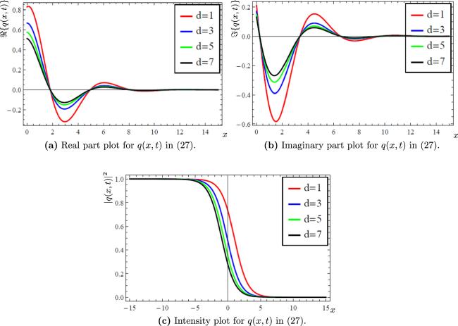
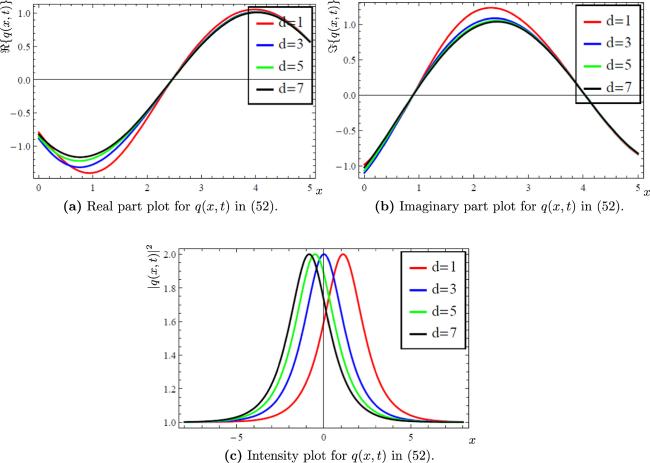
Figure 1. Influence of Kudryashov's index d on the Set-I solution in ( |
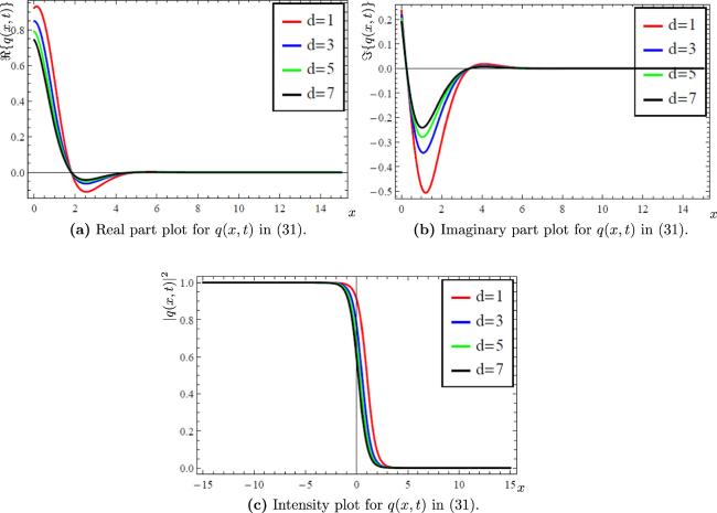
Figure 2. Influence of Kudryashov's index d on the Set-I solution in ( |
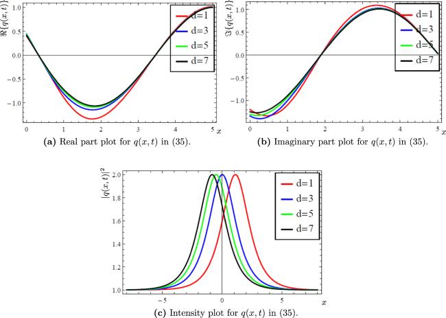
Figure 3. Influence of Kudryashov's index d on the Set-I solution in ( |

Figure 4. Influence of Kudryashov's index d on the Set-I solution in ( |
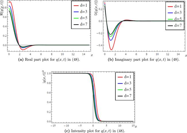
Figure 5. Influence of Kudryashov's index d on the Set-I solution in ( |
Figure 6. Influence of Kudryashov's index d on the Set-I solution in ( |