The (2 + 1)-dimensional generalized fifth-order KdV (2GKdV) equation is revisited via combined physical and mathematical methods. By using the Hirota perturbation expansion technique and via setting the nonzero background wave on the multiple soliton solution of the 2GKdV equation, breather waves are constructed, for which some transformed wave conditions are considered that yield abundant novel nonlinear waves including X/Y-Shaped (XS/YS), asymmetric M-Shaped (MS), W-Shaped (WS), Space-Curved (SC) and Oscillation M-Shaped (OMS) solitons. Furthermore, distinct nonlinear wave molecules and interactional structures involving the asymmetric MS, WS, XS/YS, SC solitons, and breathers, lumps are constructed after considering the corresponding existence conditions. The dynamical properties of the nonlinear molecular waves and interactional structures are revealed via analyzing the trajectory equations along with the change of the phase shifts.
Yan Li, Ruoxia Yao, Senyue Lou. Novel nonlinear wave transitions and interactions for (2+1)-dimensional generalized fifth-order KdV equation[J]. Communications in Theoretical Physics, 2024, 76(12): 125003. DOI: 10.1088/1572-9494/ad70a2
1. Introduction
The study of nonlinear wave bounded state structures set off a new research upsurge in more and more fields, such as optical fiber communication, fluid mechanics, biophysics and information science [1–3]. Investigating the above problems are of great significance because they can provide valuable mathematical physics information and theoretical support for nonlinear phenomena and experimental results analysis in some scientific fields [4–7]. The types of nonlinear waves can be roughly divided into four categories: soliton, breather, lump and rogue wave. Solitons have many intriguing properties of particles and waves, reflecting common nonlinear characteristics in nature. It is a well known fact that periodicity is a very basic and important attribute of nonlinear wave propagation, originating from periodic coherence between atoms. The breather perfectly describes such a solution that is periodic in both time and space dimensions [8]. The rogue wave depicts a steep wave localized in both space and time dimensions [9]. The lump solution is constructed in many integrable models, it is a type of rational exact solution and spatially localized in certain region [10, 11]. The aforementioned nonlinear wave structures can transform each other under the particular conditions, which produce many new wave structures.
Furthermore, the phenomenon of soliton resonance has also been widely explored. Soliton resonance can cause nonlinear excitation modes such as soliton fission and fusion. It is worth noting that the resonant Y-Shaped (YS) solitons actually describe the fusion and fission phenomenon of soliton, while the X-Shaped (XS) solitons can be used to describe different interaction modes under specific constraints [12, 13]. As a special case of soliton fission and fusion phenomena, Space-Curved (SC) solitons can be used to describe common curved waves in shallow water waves [14]. Researchers conducted in-depth studies on the nonlinear wave structure and asymptotic analysis of n-component nonlinear Schrödinger (n-NLS) equation with non-zero boundary/mixed boundary conditions. These findings have vital significance for understanding multi-component nonlinear physics [15, 16, 17]. In addition, the propagation of light pulses in laser systems is effectively described by introducing the generalized fractional nonlinear Schrödinger equation and constructing its basic solitons through the variational approximation method [18].
Several bounded (coherent) states of solitons including soliton molecules (SMs) and breather molecules (BMs) have been a hot topic as they can provide application and extensive theory values in nonlinear physics fields [19–21]. The velocity resonance involved in this article specifically includes two conditions: the trajectory equations of nonlinear wave components are parallel, and further, their propagation velocities are equal. Thus, multifarious novel kinds of the SMs and BMs have been constructed successively via utilizing velocity resonance. Therefore, the interactional solutions among different types of nonlinear waves have been deeply investigated, because the collision behaviors can be utilized to accurately imitate nonlinear behaviors in nature, from this point of view, the elastic collision and inelastic collision modes, the emergence and degradation behaviors of solitons, and the oscillatory and non-oscillatory modes have been carefully studied. It can be seen from the above that investigating nonlinear waves and their interactions can increase the richness of analytical solutions for nonlinear integrable systems and offer vital insights into the understanding and application of complex nonlinear integrable systems and corresponding complex nonlinear phenomena. Nevertheless, there are few investigations on the interactional structures among novel kinds of nonlinear molecular waves, resonance soliton solutions and breathers, especially the collision-free interaction modes, which arouses our interest to explore this kind solution in another model.
In this paper, we consider the (2+1)-dimensional generalized fifth-order KdV (2GKdV) equation
where α, β, γ and δ are real constant coefficients of the dispersion term and higher-order derivative terms in 2GKdV equation, respectively. Equation (1) demonstrates the behaviors of the long wave under gravity and in a two-dimensional nonlinear lattice in shallow water [22–24]. Equation (1) could convert into the (1+1)-dimensional Sawada–Kotera equation [25, 26] via removing the derivative term uy and setting α = 1, β = 15, γ = 15 and δ = 45. There are numerous studies that have focused on the 2GKdV equation, such as the lump wave and interaction structures of equation (1) were acquired in [27], complexitons and periodic soliton solutions were also studied in [28]; nonlinear superposition phenomena between lump solitons and other forms of nonlinear localized waves were examined in [29] and the lump-periodic, breather and two-soliton solutions were presented in [30].
The article is structured as follows. In section 2, we first revisit the N-soliton solution for the 2GKdV equation via the Hirota perturbation expansion method, then obtain the first-order breather, XS soliton and lump wave of the 2 GKdV equation. Next, we analyze the dynamics of the breather, XS soliton and lump wave. Moreover, we present a new class of transformed wave conditions to construct different nonlinear wave structures such as the asymmetric M-Shaped (MS) soliton, the XS/YS soliton, the Oscillation M-Shaped (OMS) soliton, the SC soliton and lattice periodic soliton, etc. In section 3, new types of molecule structures and interactional structures are constructed via the velocity resonance ansatz. We also demonstrate the dynamical properties of the above nonlinear wave structures. Finally, section 4 contains a brief summary.
2. The X-Shaped soliton, breather, lump and other types of nonlinear waves
According to [27, 31], we adopt the following bilinear transformation under the conditions that β = 15α, γ = 45α, δ = 15α and
where Dx, Dy and Dt represent the bilinear derivatives [32].
We first give the multiple soliton solutions of the 2 GKdV equation by the Hirota perturbation expansion method, then the first-order breather solution is constructed by setting partial parameters to be paired-complex conjugate forms [33], and the lump wave is created via the long-wave limit method [34, 35]. The N-soliton solution of the 2 GKdV equation is of the form
where τi, Aij represent phases and phase shifts of solitons, respectively. Besides, ki, li, φi(i = 1, 2,…,N) are arbitrary real constants; ∑μ=0,1 is the summation over possible combinations of μi, μj = 0, 1(i, j = 1, 2,…,N); the summation ${\sum }_{i\lt j}^{N}$ should take all possible pairs selected from (i, j = 1, 2,…,N).
2.1. X-Shaped soliton and first-order breather
From the expression (5), the two-soliton of equation (1) is
where ${\tau }_{1},{\tau }_{2},{{\rm{e}}}^{{A}_{12}}$ are determined by equation (6).
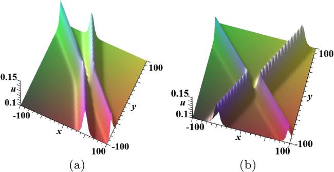
To construct the XS solitons, we further take the above two-soliton solution (7) as an example to explore the generation mechanism of XS soliton solution. By setting A12 ≫ 1 or A12 ≪ 1 in solution (7), we derive some XS solitons. Figure 1 displays the XS solitons based on solution (7). In fact, these XS solitons can describe different mutual collision modes when A12 = O(1), A12 ≫ 1 or A12 ≪ 1.
Figure 1. (a) The XS soliton given by (12) with k1 = 0.32, k2 = 0.3, l1 = 0.5, l2 = 1, α = 1, u0 = 0.1, φ1 = 0, φ2 = 0, t = 0. (b) The XS soliton given by (12) with k1 = − 0.32, k2 = 0.3, l1 = − 0.5, l2 = 1, α = 1, u0 = 0.1, φ1 = 0, φ2 = 0, t = 0.
In order to better study the superposition mechanism among nonlinear waves, we start with the first-order breather solution and some parameters are chosen as
where the asterisk (*) represents the complex conjugation and m1, n1, p1, q1, γ1, η1, λ1 denote arbitrary constants, i is the imaginary unit. Substituting equation (8) into equation (7), we suggest the function f = f(x, y, t) having the following appropriate form [36, 37]
Carrying equation (11) into the transformation $u={u}_{0}+2\mathrm{ln}{({f}_{2})}_{{xx}}$, the first-order breather solution of the 2 GKdV equation can be obtained
with ${r}_{1}=8{\lambda }_{2}{m}_{1}^{2}-2{\lambda }_{1}^{2}{n}_{1}^{2},{r}_{2}=4{\lambda }_{1}\sqrt{{\lambda }_{2}}({m}_{1}^{2}-{n}_{1}^{2}),{r}_{3}\,=8{\lambda }_{1}\sqrt{{\lambda }_{2}}{m}_{1}{n}_{1}$ and u0 being a constant background wave, which has also been presented in [38, 39].
From the above simplified expression, we find that the breather solution is composed of hyperbolic functions $H=\left\{\cosh ({\xi }_{1}-\tfrac{1}{2}\mathrm{ln}{\lambda }_{2}),\sinh ({\xi }_{1}-\tfrac{1}{2}\mathrm{ln}{\lambda }_{2})\right\}$ and trigonometric functions $T=\left\{\cos {\zeta }_{1},\sin {\zeta }_{1}\right\}$, which play essential roles in deciding the key properties of solution (12). The functions H and T reveal the localization and periodicity of the evolution process, respectively. Thus, the breather is actually a mixed solution component of the solitary-type wave and periodic-type wave. It describes the localized solutions with breathing oscillation behavior on the constant background u0. Furthermore, the propagation velocity vector of the solitary wave ${{\boldsymbol{v}}}_{{\xi }_{{\bf{1}}}}$ and propagation velocity vector of the periodic wave ${{\boldsymbol{v}}}_{{\zeta }_{{\bf{1}}}}$ are expressed in the following forms
where ${v}_{{\xi }_{1x}},{v}_{{\xi }_{1y}}$ denote the disseminate speed of the solitary wave in the x-axis and y-axis; ${v}_{{\zeta }_{1x}},{v}_{{\zeta }_{1y}}$ denote the disseminate speed of period wave in the x-axis and y-axis, respectively.
The periods T1 of the breather solution (12) are given by
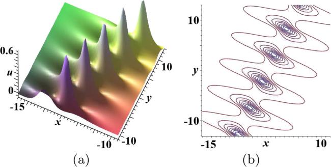
Figure 2 shows the breather solution described by equation (12) in (x,y)-plane. In figure 2, the velocities of the solitary-type wave and the periodic-type wave are ${{\boldsymbol{v}}}_{{\xi }_{{\bf{1}}}}=(0.5077,-1.0153)$ and ${{\boldsymbol{v}}}_{{\zeta }_{{\bf{1}}}}=(-3.4564,-0.9875)$, and the corresponding trajectory equations are 0.3x − 0.15y + 0.1523t = 0 and 0.3x + 1.05y − 1.0369t = 0 respectively. It should be clarified that the analytical condition to the solution (12) reads $2\sqrt{{\lambda }_{2}}\gt \left|{\lambda }_{1}\right|$.
Figure 2. The breather solution given by (12) with m1 = 0.3, n1 = 0.3, p1 = 1.5, q1 = 2, λ1 = 2, α = 1, u0 = − 0.01, γ1 = 0, η1 = 0, t = 0. (a) The spatial structure plot. (b) The contour plot of (a).
2.2. Lump-type soliton and W-Shaped soliton solutions
In the previous section, we investigate the components of the breather solution and discuss the related dynamical properties. At present, we mainly consider the lump-type wave via the long wave limit technique, namely, when ${m}_{1}^{2}+{n}_{1}^{2}\to 0$, taking the limit of the infinity period. By analyzing equations (14) and (15), we find that if the condition ${m}_{1}^{2}+{n}_{1}^{2}\to 0$ holds, the period T1 of solution (12) will tend to infinity and the breather solution as shown in figure 2 degenerates to a lump-type wave.
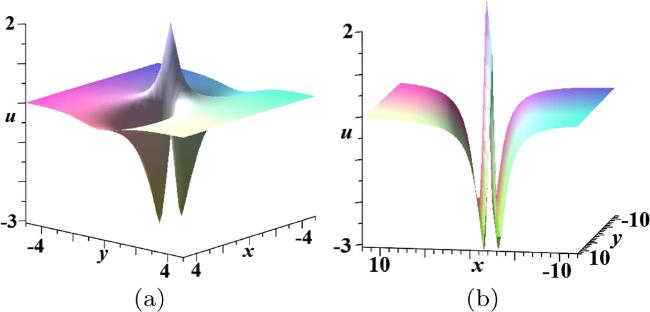
Figure 3(a) exhibits the lump-type wave with one wall-like peak and two small holes, which is localized in all directions in space [40, 41]. This solution can be viewed as ahybrid solution including a two-wave solution with variables ${\xi }_{1}^{{\prime} }=x+({p}_{1}+{q}_{1})y-({p}_{1}+{q}_{1})t$ and ${\zeta }_{1}^{{\prime} }=x\,+({p}_{1}-{q}_{1})y-({p}_{1}-{q}_{1})t$. Similar to equation (13), we can express the speeds of the two-wave solution as the forms ${\boldsymbol{}}{{\rm{v}}}_{{\xi }_{1}^{{\prime} }}=(-({p}_{1}+{q}_{1}),-1),{\boldsymbol{}}{{\rm{v}}}_{{\zeta }_{1}^{{\prime} }}=(-({p}_{1}-{q}_{1}),-1)$. The trajectory equations (${\xi }_{1}^{{\prime} }=0,{\zeta }_{1}^{{\prime} }=0$) are determined accordingly. By utilizing the extremum value theorem of function, we calculate the maximum or minimum value points of the function ulump = u(x, y, t0). It shows that the lump solution (17) possesses three extreme points at (0, t0), ( − 0.8018, t0) and (0.8018, t0) with parameters being selected as p1 = 0.5, q1 = − 2, α = 1, u0 = 0. The maximum value of lump solution (17) is 2 at (0, t0), while the minimum value is -3.0625 at (±0.8018, t0).
Figure 3. (a) The lump solution given by (17) with p1 = 0.5, q1 = − 2, α = 1, u0 = 0, t = 0. (b) The WS soliton solution given by (19) with p1 = 0.2, α = 1, u0 = 0, t = 0.
It is interesting that if we introduce a new class of parameter constraint condition that is known as the velocity resonance equation [42–44], a phenomena that the breather (12) converting into the rational WS solitary wave will occur when the following condition is satisfied, see figure 3(b).
As displayed in figure 3(b), we learn the WS soliton solution has single peak and double symmetrical valleys, of which the trajectory equation is x + 0.2(y − t) = 0.
2.3. Nonlinear wave structures from two-soliton solution (12)
In this section, we investigate the transformed wave conditions and the nonlinear wave structures including the WS solitary wave, the MS solitary wave, the OMS solitary wave and the Multi-Peak (MP) solitary wave, etc. The associated dynamic properties of the nonlinear wave structures will be studied exhaustively.
The previous investigation shows that if the direction of the propagation velocity vector ${{\boldsymbol{v}}}_{{\xi }_{{\bf{1}}}}$ of the solitary wave and the propagation velocity vector ${{\boldsymbol{v}}}_{{\zeta }_{{\bf{1}}}}$ of the periodic wave are parallel, we can obtain different types of nonlinear wave structures. In order to study the structural properties of the breather (12), we take advantage of the following condition,
That is to say, the subtle parameter condition should be met
$\begin{eqnarray}{q}_{1}=0.\end{eqnarray}$
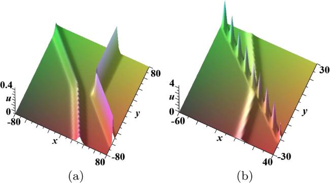
From the above analysis, we learn that the breather solution (12) component of the functions H and T possesses uniform velocity direction. The tangent of the velocity direction is expressed in the form: ${\beta }_{1}=\arctan \left({p}_{1}\right)$, where β1 is the angle between the counterclockwise direction of two velocity vectors and the positive direction of the y-axis. Hence, it is summarized that the parameter p1 is responsible for the velocity direction of the different nonlinear wave structures. A series of nonlinear localized wave structures could be constructed via the specific mechanism (21)-(23). Figure 4 displays several types of nonlinear localized waves. The WS soliton solution with single peak and double symmetric valleys $({L}_{{s}_{1}}=x+y+1.9725t=0$ and ${L}_{{p}_{1}}=1.1x+1.1y+5.6704t=0)$ is shown in figure 4(a). Next, we demonstrate three cases:
(i) When $\tfrac{{n}_{1}}{{m}_{1}}\approx 1$, an asymmetric MS soliton solution has double peaks and a valley $({L}_{{s}_{1}}=0.3x+0.3y\,-0.2967t=0$ and ${L}_{{p}_{1}}=0.2x+0.2y-0.1952t=0)$, exhibited in figure 4(b);
(ii) With the increase of value $\tfrac{{n}_{1}}{{m}_{1}}$ gradually, the MS solution will convert into the OMS soliton solution $(\tfrac{{n}_{1}}{{m}_{1}}=3.5)$, the trajectory equations ${L}_{{s}_{1}}=0.5x+0.6y+6.5152t\,=0$ and ${L}_{{p}_{1}}=1.75x+2.1y+1.065t=0$, presented in figure 4(c);
(iii) When $\tfrac{{n}_{1}}{{m}_{1}}=10$, an MP soliton solution will be obtained, as shown in figure 4(d), where the trajectory equations are ${L}_{{s}_{1}}=0.1x+0.12y+0.2495t=0$ and ${L}_{{p}_{1}}=x\,+1.2y-2.5955t=0$.
Figure 4. Spatial structure plots of the different nonlinear waves described by (12) and γ1 = 0, η1 = 0, α = 1, t = 0. (a) The WS soliton solution and m1 = 1, n1 = 1.1, p1 = 1, λ1 = 12, u0 = − 0.02. (b) The MS soliton solution and m1 = 0.3, n1 = 0.2, p1 = 1, λ1 = 2, u0 = − 0.01. (c) The OMS soliton solution and m1 = 0.5, n1 = 1.75, p1 = 1.2, λ1 = 2, u0 = 0.5. (d) The MP soliton solution and m1 = 0.1, n1 = 1, p1 = 1.2, λ1 = 2, u0 = 0.3.
To proceed, we give an analysis of the essential physical quantity, the phase shift, which has a profound impact on the dynamic behaviors of the obtained nonlinear waves. In this paper, the concrete expressions of the phase shifts of solution (12) are given by
where ${\phi }_{{\xi }_{1}}(t),{\phi }_{{\zeta }_{1}}(t)$ represent the phase shifts of the SWM and PWM, respectively, $\left|{{\boldsymbol{v}}}_{{\xi }_{{\bf{1}}}}\right|,\left|{{\boldsymbol{v}}}_{{\zeta }_{{\bf{1}}}}\right|$ denote the modulus of the velocity vectors of the SWM and PWM, ωR1, ωI1 are determined by equation (10). According to equation (24), we conclude that the phase shifts of the SWM and PWM are not equal $({\phi }_{{\xi }_{1}}(t)\ne {\phi }_{{\zeta }_{1}}(t))$ and will alter with time varying. As a result, we obtain different nonlinear wave interactional structures at different times t because the interaction regions have changed that caused by the alteration of the trajectory equation.
with ${r}_{1}=8{\lambda }_{2}{a}_{1}^{2}-2{\lambda }_{1}^{2}{a}_{2}^{2},{r}_{2}=\,4{\lambda }_{1}\sqrt{{\lambda }_{2}}({a}_{1}^{2}-{a}_{2}^{2}),{r}_{3}\,=8{\lambda }_{1}\sqrt{{\lambda }_{2}}{a}_{1}{a}_{2}$ and u0 being a constant background wave.
Similarly to expression (13), the propagation velocity vector ${{\bf{v}}}_{{\widetilde{\xi }}_{{\bf{1}}}}$ of the solitary wave and the propagation velocity vector ${{\bf{v}}}_{{\widetilde{\zeta }}_{{\bf{1}}}}$ of the periodic wave can be expressed in the following forms
If the condition ${{\boldsymbol{v}}}_{{\widetilde{\xi }}_{{\bf{1}}}}\times {{\boldsymbol{v}}}_{{\widetilde{\zeta }}_{{\bf{1}}}}={\bf{0}}$ holds, namely, b1 = b2, c1 = c2, and further letting the parameter a1 vanish, the corresponding periodic wave solution is given in the form
where ${u}_{0}=\tfrac{2{a}_{2}^{2}}{15},\tau ={a}_{2}(x+{b}_{2}y+({a}_{2}^{4}\alpha -\tfrac{4}{5}\alpha {b}_{2}{a}_{2}^{4}-{b}_{2})t)$. The existence condition for the periodic wave is $\left|\tfrac{{\lambda }_{1}}{{\lambda }_{2}+1}\right|\lt 1$. We notice that solution (29) will convert into different types of periodic structures under variant constraints about the parameters λ1, λ2.
(i) When $0\lt \left|\tfrac{{\lambda }_{1}}{{\lambda }_{2}+1}\right|\lt 1$, a sine-like periodic wave is exhibited;
(ii) when $\left|\tfrac{{\lambda }_{1}}{{\lambda }_{2}+1}\right|=\tfrac{1}{2}$, a soliton lattice with U-Shaped bottom is derived;
(iii) when $\tfrac{1}{2}\lt \left|\tfrac{{\lambda }_{1}}{{\lambda }_{2}+1}\right|\lt 1$, a soliton lattice with W-Shaped bottom is constructed.
3. Mixed solutions including YS and SC solitons and other nonlinear molecular waves
In this section, the aim is to investigate interaction structures and nonlinear molecular waves based on the mixed solution and the fourth-order soliton under the specific velocity resonance mechanism. We discuss the elastic and inelastic collision modes among the nonlinear localized wave structures. Then, we give further explanations for the inelastic collisions by the trajectory equation and the phase shift analysis.
3.1. Interaction structures from the mixed solution
Next, we focus on the Y-type soliton of the 2 GKdV equation. Taking N = 3, A12 = 0 in equations (5) and (6), the relevant resonant Y-type soliton is presented through the following expression,
and the constraints ${k}_{2}=\tfrac{1}{2}{k}_{1}\pm \tfrac{1}{2}\sqrt{-3{k}_{1}^{2}-36{u}_{0}},{u}_{0}\,\lt -\tfrac{1}{12}{k}_{1}^{2}$ should be met. Figure 5 shows the mutual collision between the YS soliton and the single soliton. The YS solitons are formed because of the resonance effect between solitons, which describes the fusion and fission phenomena between solitons. When A12 = 0, the fission phenomenon represents the splitting of one soliton into two solitons with the same structure. The fusion phenomenon represents two structurally similar solitons merging into one single soliton.
Figure 5. Spatial structure plots of the mixed solution given by (30) with α = 1, u0 = − 0.05, t = 0. (a) The interactional structure between the Y-type soliton and the single soliton with k1 = 0.5, k2 = 0.3, l1 = 0.5, l2 = 1, l3 = 0, φ1 = 0, φ2 = 0, φ3 = 0. (b) The contour plot of (a).
By introducing complex conjugation relationships to partial parameters, the well known Hirota multiple soliton solutions can be expanded to obtain the following form of mixed solution. Based on this type of solution, we can construct rich nonlinear localized waves and their interaction structures [45]. Let the detailed mixed solution expression f3 be of the form
where ξ1and ζ1 are described in expression (26). Substituting equation (31) into equation (2) leads to the interactional structure consisting of breather and soliton, which presents an elastic collision mode due to the shape of the interactional structure remaining unchanged. By applying (m1, n1) = (ε, ε), λ1 = 2, λ2 = 1 + ε2 and performing the Taylor expansion on equation (31) as ε = 0, we obtain an interactional wave structure including a lump and a soliton via appropriate parameter selections.
3.2. Interaction structures from the fourth-order solution
For the aim of constructing the space-curved resonant solitons, we assume that $\exp ({A}_{{js}})\to 0$ is true if, and only if, kj = ks, (0 < j < s ≤ 4) [46]. Introducing k1 = k2, k3 = k4 to the multiple soliton solutions (5) and (6) when N = 4 leads to the elimination of all or part of the corresponding terms $\exp ({A}_{{js}})\to 0,(0\lt j\lt s\leqslant 4)$, and f4 in $u=2{\left(\mathrm{ln}{f}_{4}\right)}_{x}$ is of the form
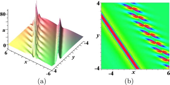
where m2, n2, p2, q2, γ2, η2 are real constants, the interaction between a space-curved soliton and a breather can be obtained. Figure 6 shows the space-curved resonant soliton interaction including the other space-curved resonant soliton/breather.
Similar to the way of obtaining the first-order breather, we can derive the second-order breather solution with condition (34). The fourth-order soliton solution is given as
where ξ1, ζ1, λ2 are defined by equation (26), and LR1, LI1 are defined by equation (32). The essential difference between the second-order breather and the first-order breather is that the former has two sets of velocity vectors $\left\{({{\boldsymbol{v}}}_{{\xi }_{{\bf{1}}}},{{\boldsymbol{v}}}_{{\zeta }_{{\bf{1}}}}),({{\boldsymbol{v}}}_{{\xi }_{{\bf{2}}}},{{\boldsymbol{v}}}_{{\zeta }_{{\bf{2}}}})\right\}$. The expressions of $({{\boldsymbol{v}}}_{{\xi }_{{\bf{2}}}},{{\boldsymbol{v}}}_{{\zeta }_{{\bf{2}}}})$ are similar to equation (13), which are given by
The ordinary second-order breather solution can be obtained under the condition that ξ1 ≠ ξ2, ζ1 ≠ ζ2 and Λ1 ≠ Λ2. We can also construct the particular second-order breather structure, i.e. the breather molecule [47–49] under the conditions ξ1 ≠ ξ2, ζ1 ≠ ζ2 and Λ1 = Λ2.
If we consider the following fixed conditions, i.e. let the parameters satisfy the conditions
then the second-order breather solution (35) transforms into a coherent structure (also called collision-free modes) of breather and soliton [50]. From figure 7, it is observed that the propagation direction of the breather and soliton are parallel, and the breather and soliton do not interfere with each other. On the other hand, we consider the following case, say, the directions of the two sets of propagation velocities are parallel
Figure 7. The breather-soliton molecule (BSM) with m1 = n1 = 1, p1 = 1, q1 = 0, m2 = n2 = 1.5, p2 = 3, q2 = 2, α = 1, λ1 = 0.75, λ3 = 2, δ1 = 5, δ2 = 0, η1 = η2 = 0, u0 = 0, t = 0. (a) The spatial structure plot. (b) The density plot of (a).
Under this case, if Λ1 ≠ Λ2(p1 ≠ p2), the molecule structure between two M-Shaped soliton (2MS) solutions is given in figure 7. On the contrary, if Λ1 = Λ2(p1 = p2), together with the above conditions (41), we can obtain a variety of nonlinear wave molecules that are composed of a bounded state of different kinds of nonlinear waves and are viewed as collision-free modes. The components of the molecules do not affect each other during the process of propagation. We show four kinds of molecule structures including the W-Shaped soliton and M-Shaped soliton (WSMS) molecule, the M-Shaped soliton and M-Shaped soliton (MSMS) molecule, the W-Shaped solitary and W-Shaped solitary (WSWS) molecule and the M-Shaped solitary and periodic soliton (MSP) molecule.
Different from the previous expressions of phase shifts (24), the phase shifts of the various interaction structures in section 3 are determined not only by the time change but also the collision of different types waves, which are given as follows
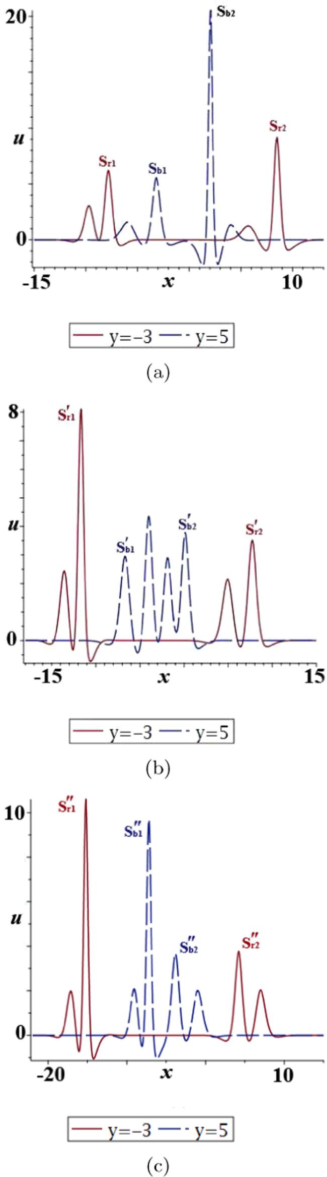
Figure 8 displays an evolution process of the 2MS molecule solution under the combined action of time and collision. The phase shift of the 2MS molecule solution is different in the evolution process, and their trajectory equations also change, which results in the change of the external waveform. When t = − 0.01, the WS soliton (Sr2) converts into WS soliton (Sb2) with a higher amplitude after interaction. When t = 0, the amplitude of the MS soliton $({{\rm{S}}}_{r1}^{{\prime} },{{\rm{S}}}_{r2}^{{\prime} })$ becomes larger, and the waveforms of both change accordingly. When t= 0.2, compared with t= 0.1, the amplitudes of the two peaks of MS solitons $({{\rm{S}}}_{r2}^{{\prime\prime} })$ exchanged. The amplitudes of the peaks of MS solitons $({{\rm{S}}}_{b1}^{{\prime\prime} })$ are greatly increased, and the amplitudes of the peaks of MS solitons $({{\rm{S}}}_{b2}^{{\prime\prime} })$ are slightly decreased.
Figure 8. The evolution diagram of the 2MS molecule interactional structure with time and m1 = 1.8, n1 = 1.6, p1 = − 1, q1 = 0, m2 = 1.5, n2 = 1, p2 = 1, q2 = 0 λ1 = 5, λ3 = 2, δ1 = 10, δ2 = 0, η1 = 10, η2 = 0, α = 1, u0 = − 0.1. (a) t = − 0.01. (b) t = 0.1. (c) y = − 3, y = 5, t = 0.2 respectively.
4. Conclusion
We investigate the 2 GKdV equation to unveil its abundant dynamic properties of related nonlinear waves while setting on a constant background wave. By introducing the paired-complex parameter restrictions and the velocity resonance conditions, we derive the breather solutions (first/second-order), lump solution, and various kinds of nonlinear waves. Furthermore, the analytic expressions of the obtained nonlinear wave structures are given, and the associated dynamic characteristics are analyzed. By using the concept of the trajectory equation of breather members (SWM and PWM) and investigating the expressions of the phase shifts, we point out the reason why the shape and amplitude of the nonlinear wave change with time. For the mixed solution and the fourth-order soliton solution, we obtain abundant interactional structures and nonlinear wave molecule solutions composed of the WSMS, MSMS, WSWS and MSP molecules. We also unearth the essence of the inelastic collision among different types of localized waves and nonlinear wave molecules via decomposing the phase shifts into a time variation part and collision part. The combined methods for investigating nonlinear wave structures to the 2 GKdV equation are also suitable to study the related nonlinear wave phenomena in other nonlinear models.
Funding was provided by the National Natural Science Foundation of China (Grant No. 12271324), the Natural Science Basic Research Program of Shaanxi Province (Grant No. 2024JC-YBQN-0069), the China Postdoctoral Science Foundation (Grant No. 2024M751921), the 2023 Shaanxi Province Postdoctoral Research Project (Grant No. 2023BSHEDZZ186), the Fundamental Research Funds for the Central Universities (Grant No. 1301032598).
MaY L2019 Interaction and energy transition between the breather and rogue wave for a generalized nonlinear Schrödinger system with two higher-order dispersion operators in optical fibers Nonlinear Dyn.97 95 105
FengY X, ZhaoZ L2024 New lump soluitons and several interaction solutions and their dynamics of a generalized (3+1)-dimensional nonlinear differential equation Commun. Theor. Phys.76 025001
PengW Q, ChenY2023 Bound-state soliton and rogue wave solutions for the sixth-order nonlinear Schrödinger equation via inverse scattering transform method Math. Meth. Appl.46 126 141
ZhangG Q, LingL M, YanZ Y2021 Multi-component nonlinear Schrödinger equations with nonzero boundary conditions: higher-order vector Peregrine solitons and asymptotic estimates J. Nonlinear Sci.31 81
ZhongM, ChenY, YanZ Y, MalomedB A2024 Suppression of soliton collapses, modulational instability and rogue-wave excitation in two-Lévy-index fractional Kerr media P. Roy. Soc. A480 20230765
ZhuangJ H, ChenX, ChuJ Y2023 Line solitons, lumps, and lump chains in the (2+1)-dimensional generalization of the Korteweg-de Vries equation Results Phys.52 106759
LiB Q, MaY L2023 Optical soliton resonances and soliton molecules for the Lakshmanan-Porsezian-Daniel system in nonlinear optics Nonlinear Dyn.111 6689 6699
BiligeS D, TemuerC L2010 An extended simplest eqaution method and its application to several forms of the fifth-order KdV eqaution Appl. Math. Comput.216 3146 3152
LüJ Q, BiligeS, ChaoluT2018 The study of lump solution and interaction phenomenon to (2+1)-dimensional generalized fifth-order KdV equation Nonlinear Dyn.91 1669 1676
TahirM, AwanA U2019 The study of complexitons and periodic solitary-wave solutions with fifth-order KdV equation in (2+1)-dimensions Mod. Phys. Lett. B33 1950411
TanW, LiuJ2020 Superposition behaviour between lump solutions and different forms of N-solitons (N → ∞ ) for the fifth-order Korteweg-de Vries equation Pramana94 36
YusufA, SulaimanT A2021 Dynamics of lump-periodic, breather and two-wave solutions with long wave in shallow water under gravity and 2D nonlinear lattice Commun. Nonliear Sci. Numer. Simulat.99 105846
YangX Y, FanR, LiB2020 Soliton molecules and some novel interaction solutions to the (2+1)-dimensional B-type Kadomtsev-Petviashvili equation Phys. Scr.95 045213
YanZ W, LouS Y2020 Special types of solitons and breather molecules for a (2+1)-dimensional fifth-order KdV equation Commun. Nonlinear Sci. Numer. Simulat.91 105425
CuiY P, WangL, GegenH2021 M-breather, M-lump, breather molecules and their interaction solutions for a (2+1)-dimensional KdV equation Phys. Scr.96 095211


