Welcome to visit Communications in Theoretical Physics,
Mathematical Physics

The extended Adomian decomposition method and its application to the rotating shallow water system for the numerical pulsrodon solutions

  • Hongli An , 1, 2, * ,
  • Liying Hou 2, * ,
  • Manwai Yuen , 3
Expand
  • 1School of Mathematics and Statistics, Nanjing University of Science and Technology, Nanjing 210094, China
  • 2College of Sciences, Nanjing Agricultural University, Nanjing 210095, China
  • 3Department of Mathematics and Information Technology, The Education University of Hong Kong, Hong Kong, China

*Author to whom any correspondence should be addressed.

Received date: 2024-03-14

  Revised date: 2024-05-27

  Accepted date: 2024-07-25

  Online published: 2024-10-22

Copyright

© 2024 Institute of Theoretical Physics CAS, Chinese Physical Society and IOP Publishing

Abstract

The rotating shallow water system is an important physical model, which has been widely used in many scientific areas, such as fluids, hydrodynamics, geophysics, oceanic and atmospheric dynamics. In this paper, we extend the application of the Adomian decomposition method from the single equation to the coupled system to investigate the numerical solutions of the rotating shallow water system with an underlying circular paraboloidal basin. By introducing some special initial values, we obtain interesting approximate pulsrodon solutions corresponding to pulsating elliptic warm-core rings, which take the form of realistic series solutions. Numerical results reveal that the numerical pulsrodon solutions can quickly converge to the exact solutions derived by Rogers and An, which fully shows the efficiency and accuracy of the proposed method. Note that the method proposed can be effectively used to construct numerical solutions of many nonlinear mathematical physics equations. The results obtained provide some potential theoretical guidance for experts to study the related phenomena in geography, oceanic and atmospheric science.

Cite this article

Hongli An , Liying Hou , Manwai Yuen . The extended Adomian decomposition method and its application to the rotating shallow water system for the numerical pulsrodon solutions[J]. Communications in Theoretical Physics, 2024 , 76(12) : 125004 . DOI: 10.1088/1572-9494/ad674f

1. Introduction

Solutions of nonlinear partial differential equations (PDEs) are important for experts to study physical phenomena. It is not only because they can help experts understand the physical phenomena described in nature, but also because they can serve as benchmarks for testing and improving numerical codes. To obtain solutions of nonlinear PDEs, many powerful methods have been proposed, such as the inverse scattering theory [1], Darboux and Bäcklund transformation [24], Adomian decomposition method (ADM) [59], Lie-group method [10], Hirota bilinear method [11, 12], variable separation approach [13, 14], Riemann–Hilbert method [1520] etc [2127]. Among these methods, the ADM is one of the most popular algorithms commonly used to construct numerical solutions and even closed-form analytical solutions. Compared to the traditional methods mentioned above, the most obvious advantage of the ADM is that it usually provides more realistic series solutions while no special assumptions or perturbation techniques are required.
In the present study, we extend the application of the ADM from the single equation to the coupled system to investigate the numerical solutions of the (2+1)-dimensional rotating shallow water (RSW) system with an underlying circular paraboloidal basin, which is described by,
$\begin{eqnarray}\left\{\begin{array}{l}\displaystyle \frac{\partial h}{\partial t}+{\bf{div}}(h{\boldsymbol{q}})=0,\\ \displaystyle \frac{\partial {\boldsymbol{q}}}{\partial t}+{\boldsymbol{q}}\cdot {\rm{\nabla }}{\boldsymbol{q}}+f{\boldsymbol{k}}\times {\boldsymbol{q}}+{\rm{\nabla }}(Z+h)=0,\end{array}\right.\end{eqnarray}$
where
$\begin{eqnarray}Z={A}^{* }({x}^{2}+{y}^{2}),\ \ \ {A}^{* }\gt 0\end{eqnarray}$
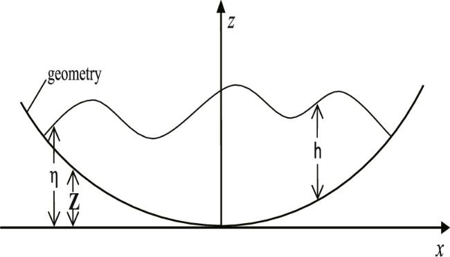
is the circular paraboloidal rigid basin, q = (u, v) is a vector of the fluid velocity, f is the Coriolis parameter and h represents the upper-layer height function scaled by a fixed height H. The free surface of the liquid is determined by,
$\begin{eqnarray}z=\eta (x,y,t)=Z+h(x,y,t).\end{eqnarray}$
All quantities are described pictorially in figure 1.
Figure 1. Cross-section of the fluid basin z = Z(x, y). h denotes the height from the free surface to the basin and η(x, y, t) = Z + h.
It is known that the RSW system is an important physical model, which has been widely used in many scientific fields, such as fluids, hydrodynamics, geophysics, oceanic and atmospheric dynamics [2832]. Due to its significance and wide applications, many scholars have paid much attention to the RSW system and numerous interesting results have been achieved. For instance, Ball obtained key results on the time evolution of moments of inertia and invariance properties of the RSW system [33, 34]. Levi and his co-authors found that by subjecting the RSW system with a circular cylindrical bottom topography to a comprehensive Lie-group analysis, some group-invariant solutions were isolated [35]. Rogers derived the complete solutions of the RSW model via an elliptical-vortex ansatz [36]. In particular, a novel subclass of so-called pulsrodon solutions was presented, which combined the pulsating characteristic of the circular pulson with the more general elliptic geometry of the rodon. Interestingly, when Holm reconsidered the RSW system in Lagrangian coordinates, he also obtained the pulsrodon solution but by using the method of Hamiltonian mechanics. Meanwhile, he found that these pulsrodons were orbitally Lyapunov stable to perturbations within the class of elliptical-vortex solutions [37]. Recently, Rogers and An have shown that the RSW system with an underlying circular paraboloidal basin admits an integrable Ermakov–Ray–Reid structure of Hamiltonian type. With the aid of the Ermakov invariant, the pulsrodons are also remarkably obtained [38]. The pulsrodons are very useful in the study of tidal oscillations, warm-core rings, oceanic and atmospheric dynamics [36, 3944]. Furthermore, the existence of the pulsrodons proves to be an important factor affecting typhoon intensity [44]. It needs to be pointed out is that the pulsrodons derived in [38] are analytical. However, to the best of our knowledge, there has been no work done on the numerical pulsrodons of the RSW equations until now. In addition, to date, there has been no related work that has been carried using the ADM. Based on the above analysis as well as the importance and wide applications of the pulsrodons and RSW system, it seems worthwhile to investigate whether numerical pulsrodons can be constructed in the RSW system via the ADM. If so, it would be of interest to apply these solutions to explain or predict some physical phenomena. In particular, it may provide some new perspectives to investigate other related phenomena in the ocean and atmosphere.
In summary, the main purpose of this paper is to extend the application of the ADM from the single equation to the coupled system to seek the numerical pulsrodons for the (2+1)-dimensional RSW system. This paper is arranged as follows. In section 2, some basic descriptions of the extended ADM for the coupled system are given. In section 3, some special initial conditions are introduced and the numerical pulsrodon solutions are constructed using the proposed method. Numerical figures show that these solutions are rotational and their behavior coincides with the motion of the ‘breather-type' oscillations of upper free surfaces in the ocean. In addition, error analysis reveals that our solutions have perfect convergence. The paper ends with a brief conclusion.

2. Description of the extended ADM

In this section, we extend the Adomain decomposition from the single equation to the coupled system. It is described as follows. Consider the nonlinear coupled differential equations in an operator form:
$\begin{eqnarray}\left\{\begin{array}{l}{\rm{L}}u+{R}_{1}(u,v,h)+{N}_{1}(u,v,h)+{g}_{1}=0,\\ {\rm{L}}v+{R}_{2}(u,v,h)+{N}_{2}(u,v,h)+{g}_{2}=0,\\ {\rm{L}}h+{R}_{3}(u,v,h)+{N}_{3}(u,v,h)+{g}_{3}=0,\end{array}\right.\end{eqnarray}$
where L is the highest-order derivative operator and its inverse can be easily solved, Ri (i = 1, 2, 3) stand for the linear differential operators with respect to u, v and h and its order is less than L, while Ni denote the nonlinear terms and gi are the source terms of the given coupled system.
After applying the inverse operator L−1 on both sub-equations of equation (4), we obtain:
$\begin{eqnarray}\left\{\begin{array}{l}u={f}_{1}(x,y,t)-{{\rm{L}}}^{-1}{g}_{1}-{{\rm{L}}}^{-1}[{R}_{1}(u,v,h)+{N}_{1}(u,v,h)],\\ v={f}_{2}(x,y,t)-{{\rm{L}}}^{-1}{g}_{2}-{{\rm{L}}}^{-1}[{R}_{2}(u,v,h)+{N}_{2}(u,v,h)],\\ h={f}_{3}(x,y,t)-{{\rm{L}}}^{-1}{g}_{3}-{{\rm{L}}}^{-1}[{R}_{3}(u,v,h)+{N}_{3}(u,v,h)],\end{array}\right.\end{eqnarray}$
where fi(x, y, t) are the functions arising from the given initial conditions. It is necessary to point out that if L is a k-order differential operator, then L−1 will be a k-fold integral with ${{\rm{L}}}^{-1}{\rm{L}}u=u(x,y,t)-u(x,y,0)-\displaystyle \sum _{j=1}^{k-1}\displaystyle \frac{1}{j!}{t}^{j}{u}_{{jt}}(x,y,0)$. Accordingly, the function f1 given in (5) is described by,
$\begin{eqnarray}{f}_{1}(x,y,t)=\left\{\begin{array}{l}u(x,y,0),\quad \quad \quad \quad \quad \quad \quad \quad \quad \quad k=1,\\ u(x,y,0)+\displaystyle \sum _{j=1}^{k-1}\displaystyle \frac{1}{j!}{t}^{j}{u}_{{jt}}(x,y,0),\quad k\geqslant 2.\end{array}\right.\end{eqnarray}$
In a similar way, one can readily write the expressions of v and h.
According to the ADM [57], the unknown solutions are described by infinite series in the following form:
$\begin{eqnarray}\begin{array}{rcl}u(x,y,t) & = & \displaystyle \sum _{n=0}^{\infty }{u}_{n}(x,y,t),\\ v(x,y,t) & = & \displaystyle \sum _{n=0}^{\infty }{v}_{n}(x,y,t),\\ h(x,y,t) & = & \displaystyle \sum _{n=0}^{\infty }{h}_{n}(x,y,t),\end{array}\end{eqnarray}$
and the nonlinear terms Ni(u, v, h) are decomposed as,
$\begin{eqnarray}{N}_{i}(u,v,h)=\displaystyle \sum _{n=0}^{\infty }{P}_{n}^{i}(u,v,h),\quad \quad (i=1,2,3),\end{eqnarray}$
where Pin are the so-called Adomian polynomials of u, v and h and defined by,
$\begin{eqnarray}\begin{array}{l}{P}_{n}^{i}=\displaystyle \frac{1}{n!}{\left[\displaystyle \frac{{{\rm{d}}}^{n}}{{\rm{d}}{\lambda }^{n}}{N}_{i}\left(\displaystyle \sum _{k=0}^{\infty }{\lambda }^{k}{u}_{k},\displaystyle \sum _{k=0}^{\infty }{\lambda }^{k}{v}_{k},\displaystyle \sum _{k=0}^{\infty }{\lambda }^{k}{h}_{k}\right)\right]}_{\lambda =0},\\ \quad n=0,1,2,\cdots .\end{array}\end{eqnarray}$
It is noted that the Adomain polynomials Pin only depend on uk, vk and hk (k = 0, ⋯ ,n) and the summation of the subscripts in each term is equal to n. Meanwhile, these polynomials can be easily computed with the aid of Maple.
Substituting the decomposition series equations (7) and (8) into (5), we obtain the following iteration recursive formulas:
$\begin{eqnarray}\begin{array}{rcl}{u}_{0} & = & {f}_{1}(x,y,t)-{{\rm{L}}}^{-1}{g}_{1},\\ {u}_{n+1} & = & -{{\rm{L}}}^{-1}[\,{R}_{1}({u}_{n},{v}_{n},{h}_{n})+{P}_{n}^{1}\,],\,\,n\geqslant 0,\\ {v}_{0} & = & {f}_{2}(x,y,t)-{{\rm{L}}}^{-1}{g}_{2},\\ {v}_{n+1} & = & -{{\rm{L}}}^{-1}[\,{R}_{2}({u}_{n},{v}_{n},{h}_{n})+{P}_{n}^{2}\,],\,\,n\geqslant 0,\\ {h}_{0} & = & {f}_{3}(x,y,t)-{{\rm{L}}}^{-1}{g}_{3},\\ {h}_{n+1} & = & -{{\rm{L}}}^{-1}[\,{R}_{3}({u}_{n},{v}_{n},{h}_{n})+{P}_{n}^{3}\,],\,\,n\geqslant 0.\end{array}\end{eqnarray}$
It can be seen that all the components un, vn and hn can be calculated from the iteration recursive relation equation (10). Usually, the decomposition series solutions $u(x,y,t)\,={\sum }_{n\,=\,0}^{\infty }{u}_{n}(x,y,t)$, $v(x,y,t)={\sum }_{n=0}^{\infty }{v}_{n}(x,y,t)$ and $h(x,y,t)\,={\sum }_{n=0}^{\infty }{h}_{n}(x,y,t)$ rapidly converge to the real physical model. For the convergence, interested readers may refer to [5, 6].
Subsequently, we apply the extended Adomain decomposition procedure given in the above to construct the numerical solutions for the (2+1)-dimensional RSW system with an underlying circular paraboloidal basin.

3. Application of the extended ADM for the numerical pulsrodons of the RSW system

To obtain the numerical solutions of the (2+1)-dimensional RSW system, we rewrite the equation with a circular paraboloidal basin (4) in the following form:
$\begin{eqnarray}\left\{\begin{array}{l}{\rm{L}}u+{{uu}}_{x}+{{vu}}_{y}+{h}_{x}-{fv}+2{A}^{* }x=0,\\ {\rm{L}}v+{{uv}}_{x}+{{vv}}_{y}+{h}_{y}+{fu}+2{A}^{* }y=0,\\ {\rm{L}}h+{\left({uh}\right)}_{x}+{\left({vh}\right)}_{y}=0,\end{array}\right.\end{eqnarray}$
where L = ∂/∂t and its inverse is ${{\rm{L}}}^{-1}(\cdot )={\int }_{0}^{t}(\cdot ){\rm{d}}s$. For the construction of numerical pulsrodons, special initial conditions are introduced:
$\begin{eqnarray}\begin{array}{rcl}u(x,y,0) & = & \left(\displaystyle \frac{{v}_{0}}{{\omega }_{0}}+\displaystyle \frac{\alpha }{{\omega }_{0}^{2}}\cos {\phi }_{0}\right)x\\ & & +\left(\displaystyle \frac{f}{2}-\displaystyle \frac{1}{{\omega }_{0}^{2}}-\displaystyle \frac{\alpha }{{\omega }_{0}^{2}}\sin {\phi }_{0}\right)y,\\ v(x,y,0) & = & \left(\displaystyle \frac{1}{{\omega }_{0}^{2}}-\displaystyle \frac{f}{2}-\displaystyle \frac{\alpha }{{\omega }_{0}^{2}}\sin {\phi }_{0}\right)x\\ & & +\left(\displaystyle \frac{{v}_{0}}{{\omega }_{0}}-\displaystyle \frac{\alpha }{{{\omega }_{0}}^{2}}\cos {\phi }_{0}\right)y,\\ h(x,y,0) & = & \left(\displaystyle \frac{k}{2{\omega }_{0}^{4}}-\displaystyle \frac{\beta }{{\omega }_{0}^{4}}\sin {\phi }_{0}\right){x}^{2}\\ & & -\displaystyle \frac{2\beta }{{\omega }_{0}^{4}}\cos {\phi }_{0}{xy}+\left(\displaystyle \frac{k}{2{\omega }_{0}^{4}}+\displaystyle \frac{\beta }{{\omega }_{0}^{4}}\sin {\phi }_{0}\right){y}^{2}\\ & & +\displaystyle \frac{{c}_{1}}{{\omega }_{0}^{2}},\end{array}\end{eqnarray}$
where α, β, v0, ω0, φ0, k and c1 are real constants and $\alpha =\sqrt{{c}_{3}+k},\beta =\sqrt{{c}_{2}+\tfrac{1}{4}{k}^{2}}\ ({c}_{2}\lt 0)$ and $k=\displaystyle \frac{2\beta (\alpha -\beta )}{{\alpha }^{2}}$.
Applying the inverse operator L−1 to both sides of equation (11) and according to equation (5), we obtain:
$\begin{eqnarray}\left\{\begin{array}{l}u=u(x,y,0)-2{A}^{* }{xt}-{{\rm{L}}}^{-1}({h}_{x}-{fv})-{{\rm{L}}}^{-1}{N}_{1}(u,v,h),\\ v=v(x,y,0)-2{A}^{* }{yt}-{{\rm{L}}}^{-1}({h}_{y}+{fu})-{{\rm{L}}}^{-1}{N}_{2}(u,v,h),\\ h=h(x,y,0)-{{\rm{L}}}^{-1}{N}_{3}(u,v,h),\end{array}\right.\end{eqnarray}$
where Ni are the nonlinear terms that can be decomposed into infinity series form:
$\begin{eqnarray}\left\{\begin{array}{l}{N}_{1}={{uu}}_{x}+{{vu}}_{y}=\displaystyle \sum _{n=0}^{\infty }{P}_{n}^{1},\\ {N}_{2}={{uv}}_{x}+{{vv}}_{y}=\displaystyle \sum _{n=0}^{\infty }{P}_{n}^{2},\\ {N}_{3}={\left({uh}\right)}_{x}+{\left({vh}\right)}_{y}=\displaystyle \sum _{n=0}^{\infty }{P}_{n}^{3}.\end{array}\right.\end{eqnarray}$
According to (9), the Adomain polynomials Pin have the following forms:
$\begin{eqnarray}\left\{\begin{array}{l}{P}_{n}^{1}=\displaystyle \sum _{k=0}^{n}\left[{u}_{k}{u}_{(n-k)x}+{v}_{k}{u}_{(n-k)y}\right],\\ {P}_{n}^{2}=\displaystyle \sum _{k=0}^{n}\left[{u}_{k}{v}_{(n-k)x}+{v}_{k}{v}_{(n-k)y}\right],\\ {P}_{n}^{3}=\displaystyle \sum _{k=0}^{n}\left[{\left({u}_{k}{h}_{(n-k)}\right)}_{x}+{\left({v}_{k}{h}_{(n-k)}\right)}_{y}\right].\end{array}\right.\end{eqnarray}$
Substituting the decomposition series equations (13)–(14) into (7) and using the initial conditions equation (12), we obtain the following recursive formulas:
$\begin{eqnarray}\left\{\begin{array}{ll}{u}_{0}=u(x,y,0)-2{A}^{* }{xt}, & {u}_{n+1}=-{{\rm{L}}}^{-1}({h}_{{nx}}-{{fv}}_{n}+{P}_{n}^{1}\,),\\ {v}_{0}=v(x,y,0)-2{A}^{* }{yt}, & {v}_{n+1}=-{{\rm{L}}}^{-1}({h}_{{ny}}+{{fu}}_{n}+{P}_{n}^{2}\,),\\ {h}_{0}=h(x,y,0), & {h}_{n+1}=-{{\rm{L}}}^{-1}{P}_{n}^{3},\qquad n\geqslant 0.\end{array}\right.\end{eqnarray}$
The values of un+1, vn+1 and hn+1 in (16) can be iteratively obtained with the aid of symbolic computation software Maple. For simplicity, here we just give the first few terms of the decomposition series:
$\begin{eqnarray}\begin{array}{rcl}{u}_{0} & = & F(x,y)-2{A}^{* }{xt},\\ {v}_{0} & = & G(x,y)-2{A}^{* }{yt},\\ {h}_{0} & = & H(x,y),\\ {u}_{1} & = & -{{\rm{L}}}^{-1}({h}_{0x}-{{fv}}_{0}+{u}_{0}{u}_{0x}+{v}_{0}{u}_{0y})\\ & = & {\bar{F}}_{1}(x,y)t+{\bar{F}}_{2}(x,y){t}^{2}+{\bar{F}}_{3}(x,y){t}^{3},\\ {v}_{1} & = & -{{\rm{L}}}^{-1}({h}_{0y}+{{fu}}_{0}+{u}_{0}{v}_{0x}+{v}_{0}{v}_{0y})\\ & = & {\bar{G}}_{1}(x,y)t+{\bar{G}}_{2}(x,y){t}^{2}+{\bar{G}}_{3}(x,y){t}^{3},\\ {h}_{1} & = & -{{\rm{L}}}^{-1}({u}_{0}{h}_{0x}+{u}_{0x}{h}_{0}+{v}_{0}{h}_{0y}+{v}_{0y}{h}_{0})\\ & = & {\bar{H}}_{1}(x,y)t+{\bar{H}}_{2}(x,y){t}^{2},\\ {u}_{2} & = & -{{\rm{L}}}^{-1}({h}_{1x}-{{fv}}_{1}+{u}_{0}{u}_{1x}+{u}_{1}{u}_{0x}+{v}_{0}{u}_{1y}+{v}_{1}{u}_{0y})\\ & = & \displaystyle \frac{1}{2}{\bar{F}}_{4}(x,y){t}^{2}+\displaystyle \frac{1}{3}{\bar{F}}_{5}(x,y){t}^{3}+\displaystyle \frac{1}{4}{\bar{F}}_{6}(x,y){t}^{4}\\ & & +\displaystyle \frac{1}{5}{\bar{F}}_{7}(x,y){t}^{5},\\ {v}_{2} & = & -{{\rm{L}}}^{-1}({h}_{1y}+{{fu}}_{1}+{u}_{0}{v}_{1x}+{u}_{1}{v}_{0x}+{v}_{0}{v}_{1y}+{v}_{1}{v}_{0y})\\ & = & \displaystyle \frac{1}{2}{\bar{G}}_{4}(x,y){t}^{2}+\displaystyle \frac{1}{3}{\bar{G}}_{5}(x,y){t}^{3}+\displaystyle \frac{1}{4}{\bar{G}}_{6}(x,y){t}^{4}\\ & & +\displaystyle \frac{1}{5}{\bar{G}}_{7}(x,y){t}^{5},\\ {h}_{2} & = & -{{\rm{L}}}^{-1}({u}_{0}{h}_{1x}+{u}_{0x}{h}_{1}+{u}_{1}{h}_{0x}+{u}_{1x}{h}_{0}\\ & & +{v}_{0}{h}_{1y}+{v}_{0y}{h}_{1}+{v}_{1}{h}_{0y}+{v}_{1y}{h}_{0})\\ & = & \displaystyle \frac{1}{2}{\bar{H}}_{3}(x,y){t}^{2}+\displaystyle \frac{1}{3}{\bar{H}}_{4}(x,y){t}^{3}+\displaystyle \frac{1}{4}{\bar{H}}_{5}(x,y){t}^{4},\\ & & \cdots \quad \quad \quad \quad \quad \quad \cdots \quad \quad \quad \quad \quad \quad \cdots \end{array}\end{eqnarray}$
where
$\begin{eqnarray}\begin{array}{rcl}F(x,y) & = & u(x,y,0),\ G(x,y)=v(x,y,0),\\ H(x,y) & = & h(x,y,0),\\ {\bar{F}}_{1}(x,y) & = & {fG}-{{FF}}_{x}-{{GF}}_{y}-{H}_{x},\\ {\bar{G}}_{1}(x,y) & = & -{fF}-{{FG}}_{x}-{{GG}}_{y}-{H}_{y},\\ {\bar{H}}_{1}(x,y) & = & -{{FH}}_{x}-{F}_{x}H-{{GH}}_{y}-{G}_{y}H,\\ {\bar{F}}_{2}(x,y) & = & {A}^{* }({{xF}}_{x}+{{yF}}_{y}+F-{yf}),\\ {\bar{G}}_{2}(x,y) & = & {A}^{* }({{xG}}_{x}+{{yG}}_{y}+G+{xf}),\\ {\bar{H}}_{2}(x,y) & = & {A}^{* }({{xH}}_{x}+{{yH}}_{y}+2H),\\ {\bar{F}}_{3}(x,y) & = & -\displaystyle \frac{4}{3}{A}^{* 2}x,\\ {\bar{G}}_{3}(x,y) & = & -\displaystyle \frac{4}{3}{A}^{* 2}y,\\ {\bar{H}}_{3}(x,y) & = & -{\left(H{\bar{F}}_{1}+{\bar{H}}_{1}F\right)}_{x}-{\left(H{\bar{G}}_{1}+{\bar{H}}_{1}G\right)}_{y},\\ {\bar{F}}_{4}(x,y) & = & f{\bar{G}}_{1}-G{\bar{F}}_{1y}-{\bar{G}}_{1}{F}_{y}-{\left(F{\bar{F}}_{1}\right)}_{x}-{\bar{H}}_{1x},\\ \ {\bar{G}}_{4}(x,y) & = & -f{\bar{F}}_{1}-F{\bar{G}}_{1x}-{\bar{F}}_{1}{G}_{x}-{\left(G{\bar{G}}_{1}\right)}_{y}-{\bar{H}}_{1y},\\ {\bar{H}}_{4}(x,y) & = & 2{A}^{* }(x{\bar{H}}_{1x}+y{\bar{H}}_{1y}+2{\bar{H}}_{1})\\ & & -{\left(H{\bar{F}}_{2}+{\bar{H}}_{2}F\right)}_{x}-{\left(H{\bar{G}}_{2}+{\bar{H}}_{2}G\right)}_{y},\\ {\bar{F}}_{5}(x,y) & = & 2{A}^{* }(x{\bar{F}}_{1x}+y{\bar{F}}_{1y}+{\bar{F}}_{1})+f{\bar{G}}_{2}-G{\bar{F}}_{2y}\\ & & -{\bar{G}}_{2}{F}_{y}-{\left(F{\bar{F}}_{2}\right)}_{x}-{\bar{H}}_{2x},\\ {\bar{G}}_{5}(x,y) & = & 2{A}^{* }(x{\bar{G}}_{1x}+y{\bar{G}}_{1y}+{\bar{G}}_{1})-f{\bar{F}}_{2}-F{\bar{G}}_{2x}\\ & & -{\bar{F}}_{2}{G}_{x}-{\left(G{\bar{G}}_{2}\right)}_{y}-{\bar{H}}_{2y},\\ {\bar{H}}_{5}(x,y) & = & 2{A}^{* }(x{\bar{H}}_{2x}+y{\bar{H}}_{2y}+2{\bar{H}}_{2})\\ & & -{\left(H{\bar{F}}_{3}\right)}_{x}-{\left(H{\bar{G}}_{3}\right)}_{y},\\ {\bar{F}}_{6}(x,y) & = & 2{A}^{* }(x{\bar{F}}_{2x}+y{\bar{F}}_{2y}+{\bar{F}}_{2})+f{\bar{G}}_{3}-G{\bar{F}}_{3y}\\ & & -{\bar{G}}_{3}{F}_{y}-{\left(F{\bar{F}}_{3}\right)}_{x},\\ {\bar{G}}_{6}(x,y) & = & 2{A}^{* }(x{\bar{G}}_{2x}+y{\bar{G}}_{2y}+{\bar{G}}_{2})-f{\bar{F}}_{3}-F{\bar{G}}_{3x}\\ & & -{\bar{F}}_{3}{G}_{x}-{\left(G{\bar{G}}_{3}\right)}_{y},\\ {\bar{F}}_{7}(x,y) & = & 2{A}^{* }(x{\bar{F}}_{3x}+y{\bar{F}}_{3y}+{\bar{F}}_{3}),\\ {\bar{G}}_{7}(x,y) & = & 2{A}^{* }(x{\bar{G}}_{3x}+y{\bar{G}}_{3y}+{\bar{G}}_{3}).\\ & & \cdots \quad \quad \quad \quad \quad \quad \cdots \quad \quad \quad \quad \quad \quad \cdots \end{array}\end{eqnarray}$
Thus, we obtain the numerical pulsrodon solution of the RSW equation (4) in a series form:
$\begin{eqnarray}\begin{array}{l}u(x,y,t)={u}_{0}+{u}_{1}+{u}_{2}+\cdot \cdot \cdot \\ \quad =\,\left(\displaystyle \frac{{v}_{0}}{{\omega }_{0}}+\displaystyle \frac{\alpha }{{\omega }_{0}^{2}}\cos {\phi }_{0}\right)x+\left(\displaystyle \frac{f}{2}-\displaystyle \frac{1}{{\omega }_{0}^{2}}-\displaystyle \frac{\alpha }{{\omega }_{0}^{2}}\sin {\phi }_{0}\right)y\\ +({\bar{F}}_{1}-2{A}^{* }x)t+\displaystyle \frac{1}{2}(2{\bar{F}}_{2}+{\bar{F}}_{4}){t}^{2}+\displaystyle \frac{1}{3}(3{\bar{F}}_{3}+{\bar{F}}_{5}){t}^{3}\\ +\displaystyle \frac{1}{4}{\bar{F}}_{6}{t}^{4}+\displaystyle \frac{1}{5}{\bar{F}}_{7}{t}^{5}+\cdot \cdot \cdot ,\\ v(x,y,t)={v}_{0}+{v}_{1}+{v}_{2}+\cdot \cdot \cdot ,\\ \quad =\left(\displaystyle \frac{1}{{\omega }_{0}^{2}}-\displaystyle \frac{f}{2}-\displaystyle \frac{\alpha }{{\omega }_{0}^{2}}\sin {\phi }_{0}\right)x+\left(\displaystyle \frac{{v}_{0}}{{\omega }_{0}}-\displaystyle \frac{\alpha }{{\omega }^{2}}\cos {\phi }_{0}\right)y\\ +({\bar{G}}_{1}-2{A}^{* }y)t+\displaystyle \frac{1}{2}(2{\bar{G}}_{2}+{\bar{G}}_{4}){t}^{2}+\displaystyle \frac{1}{3}(3{\bar{G}}_{3}+{\bar{G}}_{5}){t}^{3}\\ \,+\displaystyle \frac{1}{4}{\bar{G}}_{6}{t}^{4}+\displaystyle \frac{1}{5}{\bar{G}}_{7}{t}^{5}+\cdot \cdot \cdot ,\\ h(x,y,t)={h}_{0}+{h}_{1}+{h}_{2}+\cdot \cdot \cdot \\ \quad =\left(\displaystyle \frac{k}{2{\omega }_{0}^{4}}-\displaystyle \frac{\beta }{{\omega }_{0}^{4}}\sin {\phi }_{0}\right){x}^{2}-\displaystyle \frac{2\beta }{{\omega }_{0}^{4}}\cos {\phi }_{0}{xy}\\ \quad +\left(\displaystyle \frac{k}{2{\omega }_{0}^{4}}+\displaystyle \frac{\beta }{{\omega }_{0}^{4}}\sin {\phi }_{0}\right){y}^{2}\\ \quad +\displaystyle \frac{{c}_{1}}{{\omega }_{0}^{2}}+{\bar{H}}_{1}t+\displaystyle \frac{1}{2}(2{\bar{H}}_{2}+{\bar{H}}_{3}){t}^{2}\\ \quad +\displaystyle \frac{1}{3}{\bar{H}}_{4}{t}^{3}+\displaystyle \frac{1}{4}{\bar{H}}_{5}{t}^{4}+\cdot \cdot \cdot .\end{array}\end{eqnarray}$
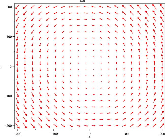
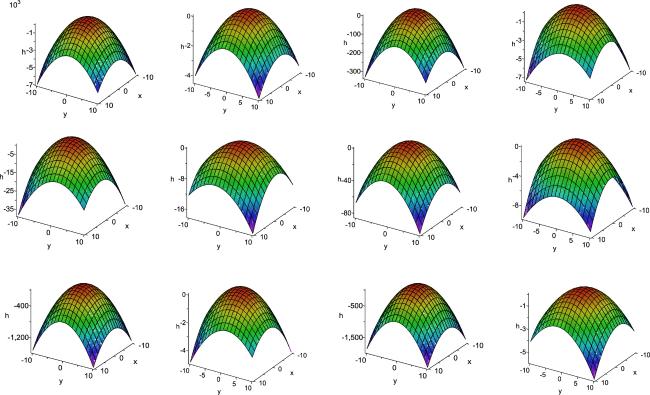
To shed some light on the behavior that the derived numerical pulsrdon solution may exhibit, we perform the numerical simulations in figures 2 and 3 wherein the parameters are chosen as α = 0.2, β = 0.4, v0 = 0.1, ω0 = 0.5, k = − 4 and c1 = 0.4. Figure 2 depicts the vortex structure of the numerical pulsrodons ${\boldsymbol{q}}=({\phi }_{n}^{u},{\phi }_{n}^{v})=(\sum _{i=0}^{n}{u}_{i},\sum _{i=0}^{n}{v}_{i})$ given by (19)1,2 with n = 2. From this figure, it can be seen that the steady fluid is rotational and the velocities of all the fluid particles go directly inwards to the origin. Figure 3 shows the time evolutions of numerical pulsrodons $h={\phi }_{n}^{h}=\sum _{i=0}^{n}{h}_{i}$ given by (19)3 with n = 2. From this figure, we find that the surface of the fluid jumps up and down over a period of time. It is of interest to note that this jumping up and down phenomenon coincides with the motion of the ‘breather-type' oscillations of upper free surfaces in the ocean [3336].
Figure 2. Structure of the velocity field ${\boldsymbol{q}}=({\phi }_{n}^{u},{\phi }_{n}^{v})$ given by (19)1,2 with n = 2. Length of the arrow represents the strength of the velocity field.
Figure 3. Time evolutions of the height function ${\phi }_{n}^{h}$ given by (19)3 with n = 2 at a regular time interval Δt = 1. Beginning time for the first sub-figure is t = 0 and the ending time for the last sub-figure is t = 11.
As known, the exact solution of the RSW equation derived by Rogers and An via an elliptic vortex procedure [38] takes the following form:
$\begin{eqnarray}\begin{array}{rcl}u(x,y,t) & = & \left(\displaystyle \frac{\dot{{\rm{\Omega }}}}{{\rm{\Omega }}}+\displaystyle \frac{\alpha }{{{\rm{\Omega }}}^{2}}\cos \phi \right)x\\ & & +\left(\displaystyle \frac{f}{2}-\displaystyle \frac{\alpha }{{{\rm{\Omega }}}^{2}}\sin \phi -\displaystyle \frac{1}{{{\rm{\Omega }}}^{2}}\right)y,\\ v(x,y,t) & = & \left(\displaystyle \frac{1}{{{\rm{\Omega }}}^{2}}-\displaystyle \frac{\alpha }{{{\rm{\Omega }}}^{2}}\sin \phi -\displaystyle \frac{f}{2}\right)x\\ & & +\left(\displaystyle \frac{\dot{{\rm{\Omega }}}}{{\rm{\Omega }}}-\displaystyle \frac{\alpha }{{{\rm{\Omega }}}^{2}}\cos \phi \right)y,\\ h(x,y,t) & = & \left(\displaystyle \frac{k}{2{{\rm{\Omega }}}^{4}}-\displaystyle \frac{\beta }{{{\rm{\Omega }}}^{4}}\sin \phi \right){x}^{2}-\displaystyle \frac{2\beta }{{{\rm{\Omega }}}^{4}}\cos \phi {xy}\\ & & +\displaystyle \frac{k}{2{{\rm{\Omega }}}^{4}}+\displaystyle \frac{\beta }{{{\rm{\Omega }}}^{4}}\sin \phi {y}^{2}+\displaystyle \frac{{c}_{1}}{{{\rm{\Omega }}}^{2}},\end{array}\end{eqnarray}$
where
$\begin{eqnarray*}\begin{array}{rcl}{\rm{\Omega }} & = & \sqrt{{\left({\omega }_{0}\cos \displaystyle \frac{1}{2}{wt}+\displaystyle \frac{2{v}_{0}}{w}\sin \displaystyle \frac{1}{2}{wt}\right)}^{2}+\displaystyle \frac{4}{{w}^{2}{\omega }_{0}^{2}}(1-{c}_{3}-2k){\sin }^{2}\displaystyle \frac{1}{2}{wt}},\\ \phi & = & {ft}-\displaystyle \frac{2\beta }{\alpha }{\int }_{0}^{t}{{\rm{\Omega }}}^{-2}{\rm{d}}\tau +{\phi }_{0},\ {\rm{\Omega }}{| }_{t=0}={\omega }_{0},\dot{{\rm{\Omega }}}{| }_{t=0}={v}_{0},w=\sqrt{{f}^{2}+8{A}^{* }}.\end{array}\end{eqnarray*}$
In order to show the efficiency and accuracy of the proposed extended ADM for the numerical solution (19), we conduct some illustrative error analysis between the first n-term approximate solution (19) and the exact solution (20) at various values. Here, we still choose the parameters to be α = 0.2, β = 0.4, v0 = 0.1, ω0 = 0.5, k = − 4 and c1 = 0.4. The differences of the numerical pulsrodons {${\phi }_{n}^{u},{\phi }_{n}^{v},{\phi }_{n}^{h}$} (n = 2) and the exact {u, v, h} are shown in tables 1, 2 and 3.
Table 1. Comparison of the numerical solution ${\phi }_{2}^{u}=\sum _{n=0}^{n=2}{u}_{n}$ given in (19)1 with the exact u(x, y, t) in (20)1 at y = 25.
x t ${\phi }_{2}^{u}$ u(x, y, t) $\left|\displaystyle \frac{u(x,y,t)-{\phi }_{2}^{u}}{u(x,y,t)}\right|$
−15 0.001 −54.92952904 −54.92828688 2.261421338e-5
−15 0.002 −55.03868175 −55.03623398 4.447560858e-5
−15 0.003 −55.14774751 −55.14413020 6.559737159e-5
−10 0.001 −55.56048101 −55.55930814 2.111023408e-5
−10 0.002 −55.63599656 −55.63361043 4.289007996e-5
−10 0.003 −55.71142341 −55.70778322 6.534437002e-5
−5 0.001 −56.19143296 −56.19373076 4.089068245e-5
−5 0.002 −56.23331135 −56.23793857 8.227933167e-5
−5 0.003 −56.27509930 −56.28208719 1.241583308e-4
Table 2. Comparison of the approximate solution ${\phi }_{2}^{v}=\sum _{n=0}^{n=2}{v}_{n}$ described in (19)2 with the exact v(x, y, t) in (20)2 at x = 50.
y t ${\phi }_{2}^{v}$ v(x, y, t) $\left|\displaystyle \frac{v(x,y,t)-{\phi }_{2}^{v}}{v(x,y,t)}\right|$
10 0.001 191.7554557 191.7508600 2.396703723e-5
10 0.002 191.8093836 191.8001286 4.825335659e-5
10 0.003 191.8628558 191.8488775 7.286099446e-5
20 0.001 197.1719901 197.1709344 5.354237445e-6
20 0.002 197.3132555 197.3110744 1.105411851e-5
20 0.003 197.4540428 197.4506662 1.710098054e-5
30 0.001 202.5885247 202.5910087 1.226115619e-5
30 0.002 202.8171274 202.8220203 2.412410641e-5
30 0.003 203.0452296 203.0524548 3.558292367e-5
Table 3. Comparison of the approximate solution ${\phi }_{2}^{h}=\sum _{n=0}^{n=2}{h}_{n}$ in (19)3 with the exact h(x, y, t) in (20)3 at y = 5.
x t ${\phi }_{2}^{h}$ h(x, y, t) $\left|\displaystyle \frac{h(x,y,t)-{\phi }_{2}^{h}}{h(x,y,t)}\right|$
20 0.001 −10883.30788 −10883.29985 7.378276911e-7
20 0.002 −10883.19728 −10883.18128 1.470158365e-6
20 0.003 −10883.38516 −10883.06243 2.965433692e-5
40 0.001 −41767.27273 −41767.36368 2.177537483e-6
40 0.002 −41767.19830 −41767.38050 4.362255852e-6
40 0.003 −41767.12281 −41767.39626 6.546972627e-6
60 0.001 −93595.76522 −93596.05893 3.138059480e-6
60 0.002 −93595.85686 −93596.44493 6.283037785e-6
60 0.003 −93595.94610 −93596.82860 9.428738272e-6
From tables 1, 2 and 3, one can easily see that although the first three terms in (19) have been chosen, the errors between numerical pulsrodon solutions (19) obtained by the extended ADM and the exact ones are rather small for different parameters, which shows that the numerical pulsrodon solutions can rapidly converge to the exact ones. In addition, numerical calculations reveal that the more terms in (19) are selected, the higher the accuracy is. Therefore, we conclude that the extended ADM is an effective method to construct numerical pulsrodons of the (2+1)-dimensional shallow water system.

4. Conclusion

In this paper, we extend the ADM from the single equation to the coupled system to investigate the numerical solutions of the 2 + 1-dimensional RSW system with a circular paraboloidal bottom basin. Remarkably, by choosing special initial conditions whose velocity components are linear and height function is quadratic, numerical pulsrodon solutions are obtained. Numerical error analysis reveals that although only a few terms in the numerical solutions are selected, the numerical solutions can rapidly converge to the exact solutions given by Rogers and An. Therefore, we conclude that the extended ADM is a very powerful algorithm to solve nonlinear differential equations, especially for the (2+1)-dimensional RSW system. However, there are still many interesting and challenging problems that need further consideration:

1. The literature shows that pulsrodons are very useful in the study of tidal oscillations, warm-core rings, oceanography, atmospheric dynamics as well as other physical areas. However, how to apply the numerical pulsrodons obtained in this paper to explain or predict some related physical phenomena needs deep investigation.

2. We know that the (2+1)-RSW system can be regarded as a model derived from the (3+1)-dimensional Euler equation via the hydrodynamic approximation. The Euler equation can be considered to be the limiting case of the Navier–Stokes equation for a large Reynolds number. Based on their connections and the importance of the Euler and Navier–Stokes equations, it would be of interest to study whether the extended ADM introduced can be adopted to construct the numerical pulsrodons of these models.

3. With the explosive growth of data and computing resources, deep learning has exhibited strong power in many fields, such as image recognition and speech recognition, especially in the scientific computation of nonlinear differential equations. It is worth considering that, when applying deep learning to the RSW system by constraining the neural networks to minimize the loss function, perhaps some predictive solutions may be obtained.

Declaration of authors

The authors declare that the authorship in the article is arranged in alphabetical order of surnames. All authors contributed equally to the work.

We express our sincere thanks to the referees for their valuable comments and helpful suggestions. This study is supported by the National Natural Science Foundation of China (Grant No. 12371250) and the Jiangsu Provincial Natural Science Foundation (Grant Nos. BK20221508, 12205154 and 11775116). As well as the Dean's Research Fund of the Education University of Hong Kong 2023/23 (FLASS/DRF/IRS-8).

1
Ablowitz M J, Clarkson P A 1991 Soliton, Nonlinear Evolution Equations and Inverse Scatting Cambridge Cambridge University Press

2
Rogers C, Schief W 2002 Bäcklund and Darboux Transformations Geometry and Modern Applications in Soliton Theory Cambridge Cambridge University Press

3
Matveev V A, Salle M A 1991 Darboux Transformations and Solitons Berlin Springer

4
Liu Q P, Manas M 2000 Darboux transformations for super-symmetric KP hierarchies Phys. Lett. B 485 293 300

DOI

5
Adomian G 1989 Nonlinear Stochastic Systems Theory and Applications to Physics Dordrecht Kluwer

6
Adomian G 1994 Solving Frontier Problems of Physics: The Decomposition Method Dordrecht Kluwer

7
Wazwaz A M 2002 Partial Differential Equations: Methods and Applications Boca Raton, FL CRC Press

8
Wazwaz A M 1995 A new approach to the nonlinear advection problem: An application of the decomposition method Appl. Math. Comput. 72 175 181

DOI

9
An H L, Chen Y 2008 Numerical solutions of a class of nonlinear evolutions with nonlinear term of any order Commun. Theor. Phys. 49 579 584

DOI

10
Bluman G W, Kumei S 1989 Symmetries and Differential Equations Berlin Springer

11
Hirota R 2004 The Direct Method in Soliton Theory Cambridge Cambridge University Press

12
Hu X B 1993 Generalized Hirota's bilinear equations and their soliton solutions J. Phys. A: Math. Gen. 26 L465 L471

DOI

13
Lou S Y, Lu J Z 1996 Special solutions from the variable separation approach: the Davey–Stewartson equation J. Phys. A: Math. Gen. 29 4209 4215

DOI

14
Lou S Y, Chen L L 1999 Formal variable separation approach for nonintegrable models J. Math. Phys. 40 6491 6500

DOI

15
Trogdon T, Deconinck B 2013 Numerical computation of the finite-genus solutions of the Korteweg–de Vries equation via Riemann–Hilbert problems Appl. Math. Lett. 26 5 9

DOI

16
Wang D S, Xu L, Xuan Z 2022 The complete classification of solutions to the Riemann problem of the defocusing complex modified KdV equation J. Nonlinear Sci. 32 3 48

DOI

17
Yang Y L, Fan E G 2023 Soliton resolution and large time behavior of solutions to the Cauchy problem for the Novikov equation with a nonzero background Adv. Math. 426 109088 86pp

DOI

18
Zhao P, Fan E G 2023 A Riemann–Hilbert method to algebro-geometric solutions of the Korteweg–de Vries equation Physica D 454 133879 24pp

DOI

19
Li Y, Tian S F, Yang J J 2022 Riemann–Hilbert problem and interactions of solitons in the n-component nonlinear Schrödinger equations Stud. Appl. Math. 148 577 605

DOI

20
Wu X, Tian S F 2023 On long-time asymptotics to the nonlocal short pulse equation with the Schwartz-type initial data: Without solitons Physica D 448 133733

DOI

21
Cao C W, Wu Y T, Geng X G 1999 Relation between the KP equation and the confocal involutive system J. Math. Phys. 40 3948 3970

DOI

22
Fan E G 2000 Extended tanh-function method and its applications to nonlinear equations Phys. Lett. A 277 212 218

DOI

23
Yan Z Y 2001 New explicit travelling wave solutions for two new integrable coupled nonlinear evolution equations Phys. Lett. A 292 100 106

DOI

24
Ma W X 2005 Complexiton solutions to integrable equations Nonlinear Anal. 63 e2461 e2471

DOI

25
Ma W X, You Y C 2005 Solving the Korteweg–de Vries equation by its bilinear form: Wronskian solutions Trans. Amer. Math. Soc. 357 1753 1778

DOI

26
Chen Y, Wang Q 2006 A unified rational expansion method to construct a series of explicit exact solutions to nonlinear evolution equations J. Appl. Math. Comput. 177 396 409

DOI

27
An H L, Feng D L 2019 General M-lump, high-order breather and localized interaction solutions to the (2 + 1)-dimensional Sawada–Kotera equation Nonlinear Dyn. 98 1275 1286

DOI

28
Paterson A R, First Course A 1983 Fluid Dynamics Cambridge Cambridge University Press

29
Lamb H 1945 Hydrodynamics Cambridge Cambridge University Press

30
Kirwan A D, Liu J 1991 The shallow water equations on an F plane Proc. Intl. School of Physics Enrico Fermi

31
Cushman-Roisin B, Heil W H, Nof D 1985 Oscillation and rotations of elliptical warm-core rings J. Geophys. Res. 90 11756 11764

DOI

32
Cushman-Roisin B 1987 Exact analytic solutions for elliptical vortices of the shallow-water equations Tellus A 39 235 244

DOI

33
Ball F K 1963 Some general theorems concerning the finite motion of a shallow liquid lying on a paraboloid J. Fluid. Mech. 17 240 256

DOI

34
Ball F K 1965 The effect of rotation on the simpler modes of motion in an elliptic paraboloid J. Fluid Mech. 22 529 545

DOI

35
Levi D, Nucci M C, Rogers C, Winternitz P 1989 Group theoretical analysis of a rotating shallow liquid in a rigid container J. Phys. A: Math. Gen. 22 4743 4767

DOI

36
Rogers C 1989 Elliptic warm-core theory: The pulsrodon Phys. Lett. A 138 267 273

DOI

37
Holm D 1991 Elliptical vortices and integrable Hamiltonian dynamics of the rotating shallow-water equations J. Fluid. Mech. 277 393 406

DOI

38
Rogers C, An H L 2010 Ermakov–Ray–Reid systems in (2+1)-dimensional rotating shallow water theory Stud. Appl. Math. 125 275 299

DOI

39
Cushman-Roisin B, Heil W H, Nof D 1985 Oscillations and rotations of elliptical warm-core rings J. Geophys. Res. 90 11756 11764

DOI

40
Rubino A, Brandt P 2003 Warm-core eddies studied by laboratory experiments and numerical modeling J. Phys. Oceanogr. 33 431 435

DOI

41
Shay L K, Goni G J, Black P G 2000 Effects of a warm oceanic feature on Hurricane Opal Mon. Weather Rev. 128 1366 1383

DOI

42
Hong X D, Chang W, Shay L K 2000 The interaction between Hurricane Opal (1995) and a warm core ring in the Gulf of Mexico Mon. Weather Rev. 128 1347 1365

DOI

43
Lou S Y, Jia M, Tang X Y, Huang F 2007 Vortices, circumfuence, symmetry groups, and Darboux transformations of the (2+1)-dimensional Euler equation Phys. Rev. E 75 056318

DOI

44
Li J Y 2010 The effect of the ocean eddy to tropical cyclone intensity The PhD dissertation of Institute of Atmospheric Sciences National Taiwan University, Taiwan

Outlines

/