Welcome to visit Communications in Theoretical Physics,
Quantum Physics and Quantum Information

Locally distinguishing genuinely nonlocal sets with entanglement resource

  • Qiao Qiao ,
  • Su-Juan Zhang , * ,
  • Chen-Ming Bai ,
  • Lu Liu
Expand
  • Department of Mathematics and Physics, Shijiazhuang Tiedao University, Shijiazhuang 050043, China

*Author to whom any correspondence should be addressed.

Received date: 2024-05-23

  Revised date: 2024-08-03

  Accepted date: 2024-08-12

  Online published: 2024-10-14

Copyright

© 2024 Institute of Theoretical Physics CAS, Chinese Physical Society and IOP Publishing. All rights, including for text and data mining, AI training, and similar technologies, are reserved.

Abstract

A set of orthogonal product states is deemed genuinely nonlocal if they remain locally indistinguishable under any bipartition. In this paper, we first construct a genuinely nonlocal product basis BI(5, 3) in ${{\mathbb{C}}}^{5}\otimes {{\mathbb{C}}}^{5}\otimes {{\mathbb{C}}}^{5}$ using a set of nonlocal product states in ${{\mathbb{C}}}^{3}\otimes {{\mathbb{C}}}^{4}$. Then, we obtain a genuinely nonlocal product basis BII(5, 3) by replacing certain states in BI(5, 3) with some superposition states. We achieve perfect discrimination of the constructed genuinely nonlocal product basis, separately employing two EPR states and one GHZ state. Our protocol is more efficient than quantum teleportation.

Cite this article

Qiao Qiao , Su-Juan Zhang , Chen-Ming Bai , Lu Liu . Locally distinguishing genuinely nonlocal sets with entanglement resource[J]. Communications in Theoretical Physics, 2024 , 76(12) : 125101 . DOI: 10.1088/1572-9494/ad6de6

1. Introduction

In the theory of quantum information, the problem of quantum state discrimination is receiving increasing attention. While a set of mutually orthogonal quantum states can always be perfectly distinguished through some global measurements, the situation is quite different when only local operations and classical communication (LOCC) are allowed. If a set of orthogonal quantum states cannot be distinguished via LOCC, then this set is termed locally indistinguishable. Locally indistinguishable quantum states have practical applications in designing quantum protocols and play significant roles in areas such as quantum voting [1], quantum data hiding [2, 3] and quantum secret sharing [46].
In 1999, Bennett et al [7] presented a set of mutually orthogonal product states in ${{\mathbb{C}}}^{3}\otimes {{\mathbb{C}}}^{3}$ that are indistinguishable under LOCC, a phenomenon they termed ‘nonlocality without entanglement'. Starting from Bennett et al, many scholars studied the nonlocality without entanglement and constructed many locally indistinguishable sets in both bipartite [813] and multipartite systems [1420]. For example, Xu et al gave a novel method to construct a nonlocal set with only 2(m + n) − 4 orthogonal product states in a ${{\mathbb{C}}}^{m}\otimes {{\mathbb{C}}}^{n}$ quantum system for nm ≥ 3 [13]. Wang et al gave an explicit construction of locally indistinguishable multipartite orthogonal product states for multipartite quantum systems by using a set of locally indistinguishable bipartite orthogonal product states [18]. In addition, Halder showed several sets of LOCC indistinguishable multipartite orthogonal product states [16].
In 2019, Halder et al [21] introduced locally irreducible sets by incorporating the property of local eliminability. Building upon this notion, they introduced strong nonlocality,where a set of orthogonal product states is considered strongly nonlocal if it remains locally irreducible in every bipartition. Strong nonlocality requires irreducibility in every bipartition, a condition that is challenging to satisfy. Naturally, the concept of genuine nonlocality without entanglement was proposed. A set of orthogonal product states in an n-partite quantum system is called genuinely nonlocal if it cannot be perfectly distinguished by any n − 1 parties collaborating through LOCC. Genuine nonlocality represents a notion stronger than nonlocality but weaker than strong nonlocality. In 2023, Xiong et al [22] proved that in the case of subsystem dimension d = 2t there exists a genuinely nonlocal set in system ${{\mathbb{C}}}^{d}\otimes {{\mathbb{C}}}^{d}\otimes {{\mathbb{C}}}^{d}$ with a cardinality of d + 3. Furthermore, in 2024, Xiong et al [23] demonstrated that, as long as condition d ≥ 4 is satisfied, there always exist d + 1 mutually orthogonal generalized GHZ states in ${{\mathbb{C}}}^{d}\otimes {{\mathbb{C}}}^{d}\otimes {{\mathbb{C}}}^{d}$, possessing genuine nonlocality.
Walgate et al [24] showed that two orthogonal pure states, entangled or otherwise, and distributed between any number of parties, can be perfectly distinguished by LOCC. Chen et al [25] showed that two nonorthogonal entangled states with equal prior probabilities can be optimally conclusively distinguished by LOCC. As widely recognized, entanglement is a valuable resource that enables communication between distant parties, as seen in applications such as quantum teleportation [26]. Locally indistinguishable quantum states may become locally distinguishable with a small amount of entanglement resources. Moreover, sets of states exhibiting such ‘nonlocality without entanglement' are connected to unextendible product bases [10]. In 2008, Cohen [27] first proposed a quantum state discrimination protocol utilizing entanglement, and the protocol is more efficient than quantum teleportation. He pointed out that certain types of unextendible product base in ${{\mathbb{C}}}^{m}\otimes {{\mathbb{C}}}^{n}$ systems can be perfectly distinguished using maximum entangled states with ⌈m/2⌉ ⨂ ⌈n/2⌉ dimensions. Subsequently, Zhang et al [28] demonstrated that certain types of orthogonal product state, which are not unextendible product bases, can be perfectly distinguished in ${{\mathbb{C}}}^{m}\otimes {{\mathbb{C}}}^{n}$ systems using entanglement as a resource. Their protocol is also more efficient than quantum teleportation. Li et al [29] introduced a method to distinguish a set of orthogonal product states in ${{\mathbb{C}}}^{d}\otimes {{\mathbb{C}}}^{d}$ systems (where d is odd) solely utilizing a single auxiliary two-qubit maximum entangled state. Then many interesting results sprang up [3034].
Rout et al [35] classified genuinely nonlocal product bases based on the local eliminability. They perfectly distinguished some genuinely nonlocal product bases in ${{\mathbb{C}}}^{3}\otimes {{\mathbb{C}}}^{3}\otimes {{\mathbb{C}}}^{3}$ and ${{\mathbb{C}}}^{4}\otimes {{\mathbb{C}}}^{4}\otimes {{\mathbb{C}}}^{4}$ using maximally entangled states. Their protocols consumed less entanglement compared to teleportation. In this work, our construction of genuinely nonlocal product basis is based on Rout's classification. We first give a set of nonlocal product states in ${{\mathbb{C}}}^{3}\otimes {{\mathbb{C}}}^{4}$, and let the states in that set make tensor products with ∣4⟩ respectively. Then, combined with the completeness of the basis, we construct a genuinely nonlocal product basis for type I in ${{\mathbb{C}}}^{5}\otimes {{\mathbb{C}}}^{5}\otimes {{\mathbb{C}}}^{5}$. Later, we briefly illustrate the genuine nonlocality of the constructed basis. Additionally, we obtain a genuinely nonlocal product basis for type II by replacing some states in type I with some superposition states. In the end, we separately employ two EPR states and one GHZ state to perfectly distinguish the genuinely nonlocal product basis for type II. In distinguishing genuinely nonlocal product basis in ${{\mathbb{C}}}^{d}\otimes {{\mathbb{C}}}^{d}\otimes {{\mathbb{C}}}^{d}$, protocols based on quantum teleportation consume 2 log2 d ebits of entanglements. Our protocols consume 2 or 1 ($\lt 2{\mathrm{log}}_{2}5$) ebits of entanglements, so ours are more efficient than quantum teleportation.
The organization of this paper is as follows. In section 2, we introduce some coherent concepts and preparatory knowledge. In section 3, we construct two types of genuinely nonlocal product basis in ${{\mathbb{C}}}^{5}\otimes {{\mathbb{C}}}^{5}\otimes {{\mathbb{C}}}^{5}$. In section 4, we perfectly distinguish the genuinely nonlocal product basis that we constructed by two EPR states and one GHZ state, respectively. In section 5, we briefly summarize this paper.

2. Preliminaries

In this section, we first introduce several relevant concepts, such as nonlocal product basis, genuinely nonlocal product basis, nontrivial orthogonality-preserving measurement and locally reducible set (see [21, 35]).

Definition 1. Suppose that $D\equiv \{| \psi {\rangle }_{j}={\displaystyle \bigotimes }_{i=1}^{n}| \alpha {\rangle }_{j}^{i}:j\,=1,\ldots ,{{\rm{\Pi }}}_{i=1}^{n}{d}_{i}\}$ is an orthogonal product basis in an n-partite quantum system ${\displaystyle \bigotimes }_{i=1}^{n}{{\mathbb{C}}}^{{d}_{i}}$.

i It is called nonlocal if states in D cannot be perfectly distinguished by LOCC.

ii It is called genuinely nonlocal if states in D cannot be perfectly distinguished by LOCC even if any $n-1$ parties are allowed to come together.

In the subsequent discussion, we suppose post-measurement states are mutually orthogonal. A measurement performed to distinguish a set of mutually orthogonal quantum states is called an orthogonality-preserving measurement if the post-measurement states remain mutually orthogonal. Furthermore, such a measurement is called trivial if all the measurement operators are proportional to the identity operator; otherwise it is nontrivial. For a nontrivial orthogonality-preserving measurement, we have the concept of locally irreducible.

Definition 2. A set of orthogonal quantum states in ${ \mathcal H }={\displaystyle \bigotimes }_{i=1}^{n}{{\mathbb{C}}}^{{d}_{i}}$ with $n\geqslant \,2$ and di $\geqslant 2$, i = 1,…,n, is locally irreducible if it is not possible to eliminate one or more states from the set by nontrivial orthogonality-preserving local measurements.

Based on the local reducibility, a genuinely nonlocal product basis can be categorized into the following types [35], and the relation is depicted in figure 1.
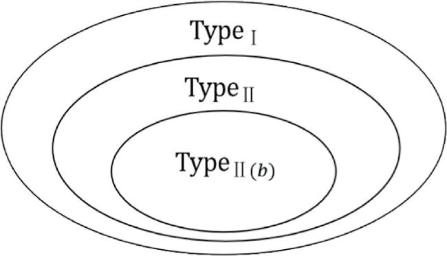
Figure 1. The relationship between several types of genuinely nonlocal product basis.
Type I: The basis of this type is locally reducible, meaning that one or more states can be eliminated under nontrivial orthogonality-preserving local measurement.
Type II: The basis of this type is locally irreducible, indicating that no states can be eliminated via nontrivial orthogonality-preserving local measurement.
Type II(a): Such a basis meets the following conditions.
(1) It is locally irreducible when participants are in different locations.
(2) Some states in it can be eliminated under nontrivial orthogonality-preserving local measurement when two of the parties come together.
Type II(b): Such a basis remains locally irreducible regardless of whether participants are in different locations or any two parties come together.

3. Genuinely nonlocal product basis in ${{\mathbb{C}}}^{5}\,\otimes \,{{\mathbb{C}}}^{5}\,\otimes \,{{\mathbb{C}}}^{5}$

In this section, we construct a genuinely nonlocal product basis BI(5, 3) from a nonlocal product basis in ${{\mathbb{C}}}^{3}\otimes {{\mathbb{C}}}^{4}$. Furthermore, we obtain genuinely nonlocal product basis BII(5, 3) by replacing certain states in BI(5, 3). In the appeal statement, BI(5, 3) represents a genuinely nonlocal product basis for type I in ${{\mathbb{C}}}^{5}\otimes {{\mathbb{C}}}^{5}\otimes {{\mathbb{C}}}^{5}$ and BII(5, 3) denotes a genuinely nonlocal product basis for type II in ${{\mathbb{C}}}^{5}\otimes {{\mathbb{C}}}^{5}\otimes {{\mathbb{C}}}^{5}$.

3.1. Genuinely nonlocal product basis for type I

We present a genuinely nonlocal product basis for type I in quantum system ${{\mathbb{C}}}^{5}\otimes {{\mathbb{C}}}^{5}\otimes {{\mathbb{C}}}^{5}$, where the computational basis for ${{\mathbb{C}}}^{5}$ will be denoted by $\{| i\rangle \}{}_{i=0}^{4}$.
First, we give a set of nonlocal quantum states in ${{\mathbb{C}}}^{3}\otimes {{\mathbb{C}}}^{4}$, denoted as
$\begin{eqnarray}{ \mathcal B }=\{| {\phi }_{1,{t}_{1}}\rangle ,| {\phi }_{2,{t}_{2}}\rangle ,| {\phi }_{3,{t}_{1}}\rangle ,| {\phi }_{4,{t}_{2}}\rangle ,| {\psi }_{\mathrm{1,1}}\rangle ,| {\psi }_{\mathrm{1,2}}\rangle \},\end{eqnarray}$
where
$\begin{eqnarray*}\begin{array}{rcl}| {\phi }_{1,{t}_{1}}\rangle & = & | 0\rangle (\displaystyle \sum _{j=0}^{2}{\omega }^{{t}_{1}j}| j\rangle );\\ | {\phi }_{2,{t}_{2}}\rangle & = & (\displaystyle \sum _{j=0}^{1}{\left(-1\right)}^{{t}_{2}j}| j\rangle )| 3\rangle ;\\ | {\phi }_{3,{t}_{1}}\rangle & = & | 2\rangle (\displaystyle \sum _{j=0}^{2}{\omega }^{{t}_{1}j}| (j+1)\rangle );\\ | {\phi }_{4,{t}_{2}}\rangle & = & (\displaystyle \sum _{j=0}^{1}{\left(-1\right)}^{{t}_{2}j}| (j+1)\rangle )| 0\rangle ;| {\psi }_{{j}_{1},{j}_{2}}\rangle =| {j}_{1}\rangle | {j}_{2}\rangle ,\\ {j}_{1},{j}_{2} & = & 0,1,2,3,4\end{array}\end{eqnarray*}$
and $\omega ={{\rm{e}}}^{\tfrac{2\pi {\rm{i}}}{3}};$ t1 = 0, 1, 2; t2 = 0, 1.
Based on the completeness of the basis, we construct
$\begin{eqnarray}\begin{array}{rcl}{{\bf{B}}}_{{\rm{I}}}(5,3) & = & \{| {\psi }_{h,i,j}\rangle ,| {\psi }_{h,4,k}\rangle ,| {\psi }_{3,k,{k}^{{\prime} }}\rangle ,| {\psi }_{4,h,4}\rangle ,| {\psi }_{4,e,k}\rangle ,\\ & & | 4\rangle | {\phi }_{1,{t}_{1}}\rangle ,| {\phi }_{1,{t}_{1}}\rangle | 4\rangle ,| 4\rangle | {\phi }_{2,{t}_{2}}\rangle ,| {\phi }_{2,{t}_{2}}\rangle | 4\rangle ,\\ & & | 4\rangle | {\phi }_{3,{t}_{1}}\rangle ,| {\phi }_{3,{t}_{1}}\rangle | 4\rangle ,| 4\rangle | {\phi }_{4,{t}_{2}}\rangle ,\\ & & | {\phi }_{4,{t}_{2}}\rangle | 4\rangle ,| 4\rangle | {\psi }_{\mathrm{1,1}}\rangle ,\\ & & | {\psi }_{\mathrm{1,1}}\rangle | 4\rangle ,| 4\rangle | {\psi }_{\mathrm{1,2}}\rangle ,| {\psi }_{\mathrm{1,2}}\rangle | 4\rangle \},\end{array}\end{eqnarray}$
where $| {\psi }_{{i}_{1},{i}_{2},{i}_{3}}\rangle =| {i}_{1}\rangle | {i}_{2}\rangle | {i}_{3}\rangle ;$ ${i}_{1},{i}_{2},{i}_{3},k,k^{\prime} =0,1,2,3,4;$ h, t1 = 0, 1, 2; i, j = 0, 1, 2, 3; e = 3, 4; t2 = 0, 1.
The set BI(5, 3) is a genuinely nonlocal product basis for type I in ${{\mathbb{C}}}^{5}\otimes {{\mathbb{C}}}^{5}\otimes {{\mathbb{C}}}^{5}$, where BI(5, 3) satisfies the following conditions.
(1) The set ${ \mathcal B }$ is a nonlocal product basis in ${{\mathbb{C}}}^{3}\otimes {{\mathbb{C}}}^{4}$, then the set of tripartite states
$\begin{eqnarray}\{| 4{\rangle }_{1}| \beta {\rangle }_{23}:| \beta \rangle \in { \mathcal B }\}\end{eqnarray}$
is locally indistinguishable in bipartite division 2∣13 as well as 3∣12, where the subscripts 1, 2 and 3 represent the first, second and third quantum systems respectively. In the same way, the set of states
$\begin{eqnarray}\{| \beta {\rangle }_{12}| 4{\rangle }_{3}:| \beta \rangle \in { \mathcal B }\}\end{eqnarray}$
is locally indistinguishable in bipartite division 1∣23 and 2∣13.
(2) Any participant can eliminate some states by performing a nontrivial orthogonality-preserving measurement. For instance, the first participant can perform a local measurement
$\begin{eqnarray}M\equiv \{| 4\rangle \langle 4| ,{{\mathbb{I}}}_{5}-| 4\rangle \langle 4| \}.\end{eqnarray}$
If the measurement outcome corresponds to ∣4⟩⟨4∣ , then the given state must be one of the following quantum states:
$\begin{eqnarray}\{| 4\rangle | \beta \rangle ,| {\psi }_{\mathrm{4,4},k}\rangle ,| {\psi }_{4,h,4}\rangle ,| {\psi }_{4,e,k}\rangle \}.\end{eqnarray}$
Otherwise, it is one of the remaining states.

3.2. Genuinely nonlocal product basis for type II

In 3.1, we constructed genuinely nonlocal product basis BI(5, 3). In order to obtain BII(5, 3), we will modify BI(5, 3) through superpositions of ∣2⟩, ∣3⟩ and ∣4⟩.
In BI(5, 3), each participant can locally eliminate some quantum states by performing a nontrivial orthogonality-preserving measurement, to distinguish the subspace spanned by ∣4⟩ from the subspace spanned by {∣0⟩, ∣1⟩, ∣2⟩, ∣3⟩}. If we prevent the local elimination of these states, we will obtain BII(5, 3).
We introduce new orthogonal product states
$\begin{eqnarray}| \tau {\rangle }_{{t}_{1}}| 4\rangle | 0\rangle ,| 3\rangle | \tau {\rangle }_{{t}_{1}}| 2\rangle ,| 1\rangle | 4\rangle | \tau {\rangle }_{{t}_{1}},\end{eqnarray}$
and use them to separately replace these states
$\begin{eqnarray}\begin{array}{rcl} & & \{| 2\rangle | 4\rangle | 0\rangle ,| 3\rangle | 4\rangle | 0\rangle ,| 4\rangle | 4\rangle | 0\rangle \},\\ & & \{| 3\rangle | 2\rangle | 2\rangle ,| 3\rangle | 3\rangle | 2\rangle ,| 3\rangle | 4\rangle | 2\rangle \},\\ & & \{| 1\rangle | 4\rangle | 2\rangle ,| 1\rangle | 4\rangle | 3\rangle ,| 1\rangle | 4\rangle | 4\rangle \},\end{array}\end{eqnarray}$
in BI(5, 3), where $| \tau {\rangle }_{{t}_{1}}\,=\,{\sum }_{j=0}^{2}{\omega }^{{t}_{1}j}| (j+2)\rangle ,{t}_{1}\,=\,0,1,2$.
In this way, any participant cannot discriminate the subspaces spanned by ∣4⟩ and {∣0⟩, ∣1⟩, ∣2⟩, ∣3⟩}, thus he or she cannot eliminate any state via nontrivial orthogonality-preserving measurement.
Therefore, we obtain that
$\begin{eqnarray}\begin{array}{l}{{\bf{B}}}_{\mathrm{II}}(5,3)={\overline{{\bf{B}}}}_{{\rm{I}}}(5,3)\,\cup \{| \tau {\rangle }_{{t}_{1}}| 4\rangle | 0\rangle ,| 3\rangle | \tau {\rangle }_{{t}_{1}}| 2\rangle ,\\ | 1\rangle | 4\rangle | \tau {\rangle }_{{t}_{1}}\}\end{array}\end{eqnarray}$
is a genuinely nonlocal product basis for type II in ${{\mathbb{C}}}^{5}\otimes {{\mathbb{C}}}^{5}\otimes {{\mathbb{C}}}^{5}$, where t1 = 0, 1, 2, and ${\overline{{\bf{B}}}}_{{\rm{I}}}(5,3)$ is denoted by
$\begin{eqnarray}\begin{array}{rcl}{\overline{{\bf{B}}}}_{{\rm{I}}}(5,3) & = & {{\bf{B}}}_{{\rm{I}}}(5,3)\setminus \{| 2\rangle | 4\rangle | 0\rangle ,| 3\rangle | 4\rangle | 0\rangle ,| 4\rangle | 4\rangle | 0\rangle ,\\ & & | 3\rangle | 2\rangle | 2\rangle ,| 3\rangle | 3\rangle | 2\rangle ,| 3\rangle | 4\rangle | 2\rangle ,\\ & & | 1\rangle | 4\rangle | 2\rangle ,| 1\rangle | 4\rangle | 3\rangle ,| 1\rangle | 4\rangle | 4\rangle \}.\end{array}\end{eqnarray}$

4. Entanglement-assisted discrimination

In this section, we distinguish the genuinely nonlocal product basis in ${{\mathbb{C}}}^{5}\otimes {{\mathbb{C}}}^{5}\otimes {{\mathbb{C}}}^{5}$ using entangled states as a resource. Suppose the states in space ${{\mathbb{C}}}^{5}\otimes {{\mathbb{C}}}^{5}\otimes {{\mathbb{C}}}^{5}$ are shared among Alice, Bob and Charlie.
First, we consider a genuinely nonlocal product basis for type I. The basis of this type can eliminate some states under nontrivial orthogonality-preserving measurement, and the entangled resource is determined after the elimination. As mentioned in the previous section, if the measurement outcome corresponds to ∣4⟩⟨4∣ we can obtain a subset of BI(5, 3) containing {∣4⟩AβBC}. Then entanglement needs to be shared between Bob and Charlie. Otherwise, the entanglement should be shared between Alice and Bob. A maximally entangled state with 3 ⨂ 3 dimensions shared between AB or BC is sufficient to perfectly distinguish BI(5, 3) (see [27]).
In order to achieve perfect discrimination, BII(5, 3) requires entanglement in each bipartition or three parties sharing of a three-qubit GHZ state. We now demonstrate that perfect discrimination of BII(5, 3) requires two additional EPR states or one GHZ state. In ${{\mathbb{C}}}^{5}\otimes {{\mathbb{C}}}^{5}\otimes {{\mathbb{C}}}^{5}$, the quantum teleportation protocol consumes 2 log2 5 ebits of entanglement in distinguishing BII(5, 3). We use a smaller amount of entanglement than this, so our protocol is more efficient than quantum teleportation.

Theorem 1. Suppose Alice and Bob share the maximally entangled state $\tfrac{1}{\sqrt{2}}{\left(| 00\rangle +| 11\rangle \right)}_{{a}_{1}{b}_{1}}$ and Alice and Charlie share the maximally entangled state $\tfrac{1}{\sqrt{2}}{\left(| 00\rangle +| 11\rangle \right)}_{{a}_{2}{c}_{1}}$, the set ${{\bf{B}}}_{\mathrm{II}}(5,3)$ in (9) can be perfectly distinguished by LOCC.

Proof. For the entangled state $\tfrac{1}{\sqrt{2}}{\left(| 00\rangle +| 11\rangle \right)}_{{a}_{1}{b}_{1}}$, assume that Alice takes the a1 particle and Bob takes the b1 particle, and for the entangled state $\tfrac{1}{\sqrt{2}}{\left(| 00\rangle +| 11\rangle \right)}_{{a}_{2}{c}_{1}}$, assume that Alice takes the a2 particle and Bob takes the c1 particle.

Accordingly, the initial state is

$\begin{eqnarray}\begin{array}{rcl}| \zeta \rangle & = & | \psi {\rangle }_{\mathrm{ABC}}\otimes \displaystyle \frac{1}{\sqrt{2}}{\left(| 00\rangle +| 11\rangle \right)}_{{a}_{1}{b}_{1}}\\ & & \otimes \,\displaystyle \frac{1}{\sqrt{2}}{\left(| 00\rangle +| 11\rangle \right)}_{{a}_{2}{c}_{1}},\end{array}\end{eqnarray}$
where $| \psi {\rangle }_{\mathrm{ABC}}$ is one of the states from the set ${{\bf{B}}}_{\mathrm{II}}(5,3)$.

Next, Alice, Bob and Charlie perform nontrivial orthogonality-preserving measurement separately, and the specific procedure as follows.

${\bf{Step}}\,{\bf{1}}$ Bob selects the measurement operator in ${\bf{M}}$ to measure the initial state $| \zeta \rangle $, where

$\begin{eqnarray}\begin{array}{l}{\bf{M}}\equiv \{{M}_{1}:= | 0\rangle \langle 0{| }_{B}\otimes | 0\rangle \langle 0{| }_{{b}_{1}}+(| 1\rangle \langle 1| +| 2\rangle \langle 2| \\ \,{+| 3\rangle \langle 3| +| 4\rangle \langle 4| )}_{{\rm{B}}}\otimes | 1\rangle \langle 1{| }_{{b}_{1}},\,{\bar{M}}_{1}:= {\unicode{120128}}-{M}_{1}\}.\end{array}\end{eqnarray}$
Then Charlie selects the measurement operator in ${\bf{N}}$ to measure Bob's post-measurement states, where
$\begin{eqnarray}\begin{array}{l}{\bf{N}}\equiv \{{N}_{1}:= | 0\rangle \langle 0{| }_{C}\otimes | 0\rangle \langle 0{| }_{{c}_{1}}+\left(| 1\rangle \langle 1| +| 2\rangle \langle 2| \right.\\ \,+\,| 3\rangle \langle 3| {\left.+| 4\rangle \langle 4| \right)}_{C}\otimes | 1\rangle \langle 1{| }_{{c}_{1}},\,{\overline{N}}_{1}:= {\mathbb{I}}-{N}_{1}\}.\end{array}\end{eqnarray}$
Suppose Bob selects M1 and Charlie selects N1; the post-measurement states are shown in table 1.

${\bf{Step}}\,{\bf{2}}$ Alice selects the measurement operator in ${\bf{K}}$ to measure the post-measurement states in table 1, where

$\begin{eqnarray}\begin{array}{rcl}{\bf{K}}\equiv \{{K}_{1} & := & {\left(| 1\rangle \langle 1| +| 2\rangle \langle 2| \right)}_{A}\otimes | 0\rangle \langle 0{| }_{{a}_{1}}\otimes {{\mathbb{I}}}_{{a}_{2}},\\ {K}_{2} & := & | 1\rangle \langle 1{| }_{A}\otimes | 1\rangle \langle 1{| }_{{a}_{1}}\otimes | 0\rangle \langle 0{| }_{{a}_{2}},\\ {K}_{3} & := & | 3\rangle \langle 3{| }_{A}\otimes | 0\rangle \langle 0{| }_{{a}_{1}}\otimes {{\mathbb{I}}}_{{a}_{2}},\\ {K}_{4} & := & | 2\rangle \langle 2{| }_{A}\otimes | 1\rangle \langle 1{| }_{{a}_{1}}\otimes | 1\rangle \langle 1{| }_{{a}_{2}},\\ {K}_{5} & := & | 3\rangle \langle 3{| }_{A}\otimes | 1\rangle \langle 1{| }_{{a}_{1}}\otimes | 1\rangle \langle 1{| }_{{a}_{2}},\\ {K}_{6} & := & {\mathbb{I}}-{K}_{1}-{K}_{2}-{K}_{3}-{K}_{4}-{K}_{5}\}.\end{array}\end{eqnarray}$
States corresponding to the measurement operators K1, K2, K3, K4 and K5 separately are
$\begin{eqnarray*}\begin{array}{rcl}{K}_{1} & \Rightarrow & \{| 1\rangle | 0\rangle | 0\rangle ,| 2\rangle | 0\rangle | 0\rangle ,| 1\rangle | 0\rangle | f\rangle ,| 2\rangle | 0\rangle | f\rangle ,| {\phi }_{4,{t}_{2}}\rangle | 4\rangle \},\\ f & = & 1,2,3;\,{t}_{2}=0,1.\\ {K}_{2} & \Rightarrow & \{| 1\rangle | m\rangle | 0\rangle \},m=1,2,3,4.\\ {K}_{3} & \Rightarrow & \{| 3\rangle | 0\rangle | k\rangle \},k=0,1,2,3,4.\\ {K}_{4} & \Rightarrow & \{| 2\rangle | m\rangle | f\rangle ,| 2\rangle | 4\rangle | 4\rangle ,| {\phi }_{3,{t}_{1}}\rangle | 4\rangle \},\\ m & = & 1,2,3,4;\,f=1,2,3;\,{t}_{1}=0,1,2.\\ {K}_{5} & \Rightarrow & \{| 3\rangle | 1\rangle | m\rangle ,| 3\rangle | 2\rangle | l\rangle ,| 3\rangle | 3\rangle | l\rangle ,| 3\rangle | 4\rangle | l\rangle ,| 3\rangle | \tau {\rangle }_{{t}_{1}}| 2\rangle \},\\ m & = & 1,2,3,4;\,l=1,3,4;\,{t}_{1}=0,1,2.\end{array}\end{eqnarray*}$
The states in each of these sets are LOCC distinguishable. If Alice selects the measurement operator K6, the state is one of the remaining states.

After Alice's measurements, we are able to screen out some locally distinguishable sets of quantum states. The remaining quantum states are locally indistinguishable and remain unchanged. Further measurements can be performed on these remaining quantum states. This is true for every subsequent step.

${\bf{Step}}\,{\bf{3}}$ Bob selects the measurement operator in ${\bf{M}}^{\prime} $ to measure the remaining quantum states in table 1, where

$\begin{eqnarray}\begin{array}{l}{\bf{M}}^{\prime} \equiv \{{M}_{12}:= | 4\rangle \langle 4{| }_{B}\otimes {{\mathbb{I}}}_{{b}_{1}},\,{M}_{22}:= | 3\rangle \langle 3{| }_{B}\\ \,\otimes \,{{\mathbb{I}}}_{{b}_{1}},\,{M}_{32}:= {\mathbb{I}}-{M}_{12}-{M}_{22}\}.\end{array}\end{eqnarray}$
States corresponding to the measurement operators M12 and M22 separately are
$\begin{eqnarray*}\begin{array}{l}{M}_{12}\Rightarrow \{| 0\rangle | 4\rangle | k\rangle ,| 1\rangle | 4\rangle | 1\rangle ,| 4\rangle | 4\rangle | m\rangle ,\\ \,\ \ \,| 1\rangle | 4\rangle | \tau {\rangle }_{{t}_{1}},| \tau {\rangle }_{{t}_{1}}| 4\rangle | 0\rangle \},\\ k=0,1,2,3,4;\,m=1,2,3,4;\,{t}_{1}=0,1,2.\\ {M}_{22}\Rightarrow \{| 0\rangle | 3\rangle | 0\rangle ,| 2\rangle | 3\rangle | 0\rangle ,| 3\rangle | 3\rangle | 0\rangle ,| 4\rangle | 3\rangle | 0\rangle ,\\ \,\ \ \,| g\rangle | 3\rangle | f\rangle ,| 4\rangle | 3\rangle | m\rangle ,| {\phi }_{2,{t}_{2}}\rangle | 4\rangle \},\\ g=0,1;f=1,2,3;\,m=1,2,3,4;\,{t}_{2}=0,1.\end{array}\end{eqnarray*}$
The states in each of these sets are LOCC distinguishable. If Bob selects the measurement operator M32, the state is one of the remaining states.

${\bf{Step}}\,{\bf{4}}$ Alice selects the measurement operator in ${\bf{K}}^{\prime} $ to measure the remaining quantum states in table 1, where

$\begin{eqnarray}\begin{array}{rcl}{\bf{K}}^{\prime} & \equiv & \{{K}_{12}:= | 1\rangle \langle 1{| }_{A}\otimes {{\mathbb{I}}}_{{a}_{1}}\otimes {{\mathbb{I}}}_{{a}_{2}},\\ {K}_{22} & := & | 4\rangle \langle 4{| }_{A}\otimes | 1\rangle \langle 1{| }_{{a}_{1}}\otimes | 0\rangle \langle 0{| }_{{a}_{2}},\\ {K}_{32} & := & | 0\rangle \langle 0{| }_{A}\otimes {{\mathbb{I}}}_{{a}_{1}}\otimes | 1\rangle \langle 1{| }_{{a}_{2}},\\ {K}_{42} & := & {\left(| 0\rangle \langle 0| +| 2\rangle \langle 2| +| 3\rangle \langle 3| \right)}_{A}\otimes | 1\rangle \langle 1{| }_{{a}_{1}}\otimes | 0\rangle \langle 0{| }_{{a}_{2}},\\ {K}_{52} & := & {\mathbb{I}}-{K}_{12}-{K}_{22}-{K}_{32}-{K}_{42}\}.\end{array}\end{eqnarray}$
States corresponding to the measurement operators K12, K22, K32 and K42 separately are
$\begin{eqnarray*}\begin{array}{rcl}{K}_{12} & \Rightarrow & \{| 1\rangle | 1\rangle | f\rangle ,| 1\rangle | 2\rangle | f\rangle ,| {\psi }_{\mathrm{1,1}}\rangle | 4\rangle ,| {\psi }_{\mathrm{1,2}}\rangle | 4\rangle \},\\ f & = & 1,2,3.\\ {K}_{22} & \Rightarrow & \{| 4\rangle | {\phi }_{4,{t}_{2}}\rangle \},{t}_{2}=0,1.\\ {K}_{32} & \Rightarrow & \{| 0{\rangle }_{{\rm{A}}}[| 0{\rangle }_{{\rm{B}}}\otimes | 00{\rangle }_{{a}_{1}{b}_{1}}+{\omega }^{{t}_{1}}| 1\rangle \\ & & {+\,{\omega }^{2{t}_{1}}| 2\rangle }_{{\rm{B}}}\otimes | 11\rangle {a}_{1}{b}_{1}]| 4{\rangle }_{{\rm{C}}}\otimes | 11{\rangle }_{{a}_{2}{c}_{1}},| 0\rangle | h\rangle | f\rangle \},\\ h & = & 0,1,2;\,f\,=\,1,2,3;\,{t}_{1}\,=\,0,1,2;\,\omega ={{\rm{e}}}^{\tfrac{2\pi {\rm{i}}}{3}}.\\ {K}_{42} & \Rightarrow & \{| 0\rangle | 1\rangle | 0\rangle ,| 0\rangle | 2\rangle | 0\rangle ,\\ & & | 2\rangle | 1\rangle | 0\rangle ,| 2\rangle | 2\rangle | 0\rangle ,| 3\rangle | 1\rangle | 0\rangle ,| 3\rangle | 2\rangle | 0\rangle \}.\end{array}\end{eqnarray*}$
The states in each of these sets are LOCC distinguishable. If Alice selects the measurement operator K52, the state is one of the remaining states.

${\bf{Step}}\,{\bf{5}}$ Bob selects the measurement operator in ${\bf{M}}^{\prime\prime} $ to measure the remaining quantum states in table 1, where

$\begin{eqnarray}\begin{array}{rcl}{\bf{M}}^{\prime\prime} & \equiv & \{{M}_{13}:= | 2\rangle \langle 2{| }_{{\rm{B}}}\otimes {{\unicode{120128}}}_{{b}_{1}},\\ \,{M}_{23} & := & {\left(| 0\rangle \langle 0| +| 1\rangle \langle 1| \right)}_{{\rm{B}}}\otimes {{\unicode{120128}}}_{{b}_{1}},\,{M}_{33}:= {\unicode{120128}}-{M}_{13}-{M}_{23}\}.\end{array}\end{eqnarray}$
States corresponding to the measurement operators M13 and M23 are
$\begin{eqnarray*}\begin{array}{rcl}{M}_{13} & \Rightarrow & \{| 4\rangle | 2\rangle | 4\rangle ,| 4\rangle | {\phi }_{3,{t}_{1}}\rangle \},\,{t}_{1}=0,1,2.\\ {M}_{23} & \Rightarrow & \{| 0\rangle | 0\rangle | 0\rangle ,| 4\rangle | 0\rangle | 4\rangle ,| 4\rangle | 1\rangle | 4\rangle ,| 4\rangle | {\psi }_{\mathrm{1,1}}\rangle ,| 4\rangle | {\psi }_{\mathrm{1,2}}\rangle ,\\ & & | 4{\rangle }_{\rm{A}}| 0{\rangle }_{{\rm{B}}}[| 0{\rangle }_{{\rm{C}}}\otimes | 00{\rangle }_{{a}_{2}{c}_{1}}{\left({\omega }^{{t}_{1}}| 1\rangle +{\omega }^{2{t}_{1}}| 2\rangle \right)}_{{\rm{C}}}\otimes | 11{\rangle }_{{a}_{2}{c}_{1}}]\\ & & \otimes | 00{\rangle }_{{a}_{1}{b}_{1}},\\ & & | 4{\rangle }_{{\rm{A}}}[| 0{\rangle }_{{\rm{B}}}\otimes | 00{\rangle }_{{a}_{1}{b}_{1}}\pm | 1{\rangle }_{{\rm{B}}}\otimes | 11{\rangle }_{{a}_{1}{b}_{1}}]| 3{\rangle }_{{\rm{C}}}\otimes | 11{\rangle }_{{a}_{2}{c}_{1}}\},\\ & & \omega ={{\rm{e}}}^{\tfrac{2\pi {\rm{i}}}{3}};{t}_{1}\,=\,0,1,2.\end{array}\end{eqnarray*}$
The states in each of these sets are LOCC distinguishable.

In ${\bf{Step}}\,{\bf{1}}$, if Bob selects M1 and Charlie selects ${\overline{N}}_{1}$, or other situations, there will also be a similar protocol. □

Table 1. Post-measurement states after Step 1.
Post-measurement states Range
$| i\rangle | 0\rangle | 0\rangle \otimes | 00{\rangle }_{{a}_{1}{b}_{1}}\otimes | 00{\rangle }_{{a}_{2}{c}_{1}}.$ i = 0, 1, 2, 3.

$| h\rangle | 0\rangle | f\rangle \otimes | 00{\rangle }_{{a}_{1}{b}_{1}}\otimes | 11{\rangle }_{{a}_{2}{c}_{1}},\,\,\,| 3\rangle | 0\rangle | m\rangle \otimes | 00{\rangle }_{{a}_{1}{b}_{1}}\otimes | 11{\rangle }_{{a}_{2}{c}_{1}},$ h = 0, 1, 2; f = 1, 2, 3;
$| 4\rangle | 0\rangle | 4\rangle \otimes | 00{\rangle }_{{a}_{1}{b}_{1}}\otimes | 11{\rangle }_{{a}_{2}{c}_{1}},\,\,\,\,| {\phi }_{4,{t}_{2}}\rangle | 4\rangle \otimes | 00{\rangle }_{{a}_{1}{b}_{1}}\otimes | 11{\rangle }_{{a}_{2}{c}_{1}}.$ m = 1, 2, 3, 4; t2 = 0, 1.

$| g\rangle | m\rangle | 0\rangle \otimes | 11{\rangle }_{{a}_{1}{b}_{1}}\otimes | 00{\rangle }_{{a}_{2}{c}_{1}},\,\,| 2\rangle | f\rangle | 0\rangle \otimes | 11{\rangle }_{{a}_{1}{b}_{1}}\otimes | 00{\rangle }_{{a}_{2}{c}_{1}},$ g, t2 = 0, 1;
$| 3\rangle | f\rangle | 0\rangle \otimes | 11{\rangle }_{{a}_{1}{b}_{1}}\otimes | 00{\rangle }_{{a}_{2}{c}_{1}},\,\,\,| 4\rangle | 3\rangle | 0\rangle \otimes | 11{\rangle }_{{a}_{1}{b}_{1}}\otimes | 00{\rangle }_{{a}_{2}{c}_{1}},$ m = 1, 2, 3, 4;
$| 4\rangle | {\phi }_{4,{t}_{2}}\rangle \otimes | 11{\rangle }_{{a}_{1}{b}_{1}}\otimes | 00{\rangle }_{{a}_{2}{c}_{1}},\,\,\,| \tau {\rangle }_{{t}_{1}}| 4\rangle | 0\rangle \otimes | 11{\rangle }_{{a}_{1}{b}_{1}}\otimes | 00{\rangle }_{{a}_{2}{c}_{1}}.$ f = 1, 2, 3; t1 = 0, 1, 2.

$| h\rangle | f\rangle | f^{\prime} \rangle \otimes | 11{\rangle }_{{a}_{1}{b}_{1}}\otimes | 11{\rangle }_{{a}_{2}{c}_{1}},\,\,| 0\rangle | 4\rangle | m\rangle \otimes | 11{\rangle }_{{a}_{1}{b}_{1}}\otimes | 11{\rangle }_{{a}_{2}{c}_{1}},$
$| 1\rangle | 4\rangle | 1\rangle \otimes | 11{\rangle }_{{a}_{1}{b}_{1}}\otimes | 11{\rangle }_{{a}_{2}{c}_{1}},\,\,\,\,| 1\rangle | 4\rangle | \tau {\rangle }_{{t}_{1}}\otimes | 11{\rangle }_{{a}_{1}{b}_{1}}\otimes | 11{\rangle }_{{a}_{2}{c}_{1}},$
$| 2\rangle | 4\rangle | m\rangle \otimes | 11{\rangle }_{{a}_{1}{b}_{1}}\otimes | 11{\rangle }_{{a}_{2}{c}_{1}},\,\,\,| 3\rangle | 1\rangle | m\rangle \otimes | 11{\rangle }_{{a}_{1}{b}_{1}}\otimes | 11{\rangle }_{{a}_{2}{c}_{1}},$
$| 3\rangle | 2\rangle | 1\rangle \otimes | 11{\rangle }_{{a}_{1}{b}_{1}}\otimes | 11{\rangle }_{{a}_{2}{c}_{1}},\,\,\,\,| 3\rangle | \tau {\rangle }_{{t}_{1}}| 2\rangle \otimes | 11{\rangle }_{{a}_{1}{b}_{1}}\otimes | 11{\rangle }_{{a}_{2}{c}_{1}},$ h, t1 = 0, 1, 2; $f,f^{\prime} =1,2,3;$
$| 3\rangle | 2\rangle | 3\rangle \otimes | 11{\rangle }_{{a}_{1}{b}_{1}}\otimes | 11{\rangle }_{{a}_{2}{c}_{1}},\,\,\,\,| 3\rangle | 2\rangle | 4\rangle \otimes | 11{\rangle }_{{a}_{1}{b}_{1}}\otimes | 11{\rangle }_{{a}_{2}{c}_{1}},$ m = 1, 2, 3, 4;
$| 3\rangle | 3\rangle | l\rangle \otimes | 11{\rangle }_{{a}_{1}{b}_{1}}\otimes | 11{\rangle }_{{a}_{2}{c}_{1}},\,\,\,\,\,| 3\rangle | 4\rangle | l\rangle \otimes | 11{\rangle }_{{a}_{1}{b}_{1}}\otimes | 11{\rangle }_{{a}_{2}{c}_{1}},$ l = 1, 3, 4;
$| 4\rangle | 1\rangle | 4\rangle \otimes | 11{\rangle }_{{a}_{1}{b}_{1}}\otimes | 11{\rangle }_{{a}_{2}{c}_{1}},\,\,\,\,| 4\rangle | 2\rangle | 4\rangle \otimes | 11{\rangle }_{{a}_{1}{b}_{1}}\otimes | 11{\rangle }_{{a}_{2}{c}_{1}},$ t2 = 0, 1.
$| 4\rangle | 3\rangle | m\rangle \otimes | 11{\rangle }_{{a}_{1}{b}_{1}}\otimes | 11{\rangle }_{{a}_{2}{c}_{1}},\,\,\,| 4\rangle | 4\rangle | m\rangle \otimes | 11{\rangle }_{{a}_{1}{b}_{1}}\otimes | 11{\rangle }_{{a}_{2}{c}_{1}},$
$| 4\rangle | {\phi }_{3,{t}_{1}}\rangle \otimes | 11{\rangle }_{{a}_{1}{b}_{1}}\otimes | 11{\rangle }_{{a}_{2}{c}_{1}},\,\,\,\,| 4\rangle | {\psi }_{\mathrm{1,1}}\rangle \otimes | 11{\rangle }_{{a}_{1}{b}_{1}}\otimes | 11{\rangle }_{{a}_{2}{c}_{1}},$
$| 4\rangle | {\psi }_{\mathrm{1,2}}\rangle \otimes | 11{\rangle }_{{a}_{1}{b}_{1}}\otimes | 11{\rangle }_{{a}_{2}{c}_{1}},\,\,\,\,\,| {\phi }_{2,{t}_{2}}\rangle | 4\rangle \otimes | 11{\rangle }_{{a}_{1}{b}_{1}}\otimes | 11{\rangle }_{{a}_{2}{c}_{1}},$
$| {\phi }_{3,{t}_{1}}\rangle | 4\rangle \otimes | 11{\rangle }_{{a}_{1}{b}_{1}}\otimes | 11{\rangle }_{{a}_{2}{c}_{1}},\,\,\,\,| {\psi }_{\mathrm{1,1}}\rangle | 4\rangle \otimes | 11{\rangle }_{{a}_{1}{b}_{1}}\otimes | 11{\rangle }_{{a}_{2}{c}_{1}},$
$| {\psi }_{\mathrm{1,2}}\rangle | 4\rangle \otimes | 11{\rangle }_{{a}_{1}{b}_{1}}\otimes | 11{\rangle }_{{a}_{2}{c}_{1}}.$

$| 4{\rangle }_{{\rm{A}}}| 0{\rangle }_{{\rm{B}}}[| 0{\rangle }_{{\rm{C}}}\otimes | 00{\rangle }_{{a}_{2}{c}_{1}}+{\left({\omega }^{{t}_{1}}| 1\rangle +{\omega }^{2{t}_{1}}| 2\rangle \right)}_{{\rm{C}}}\otimes | 11{\rangle }_{{a}_{2}{c}_{1}}]\otimes | 00{\rangle }_{{a}_{1}{b}_{1}},$
$| 4{\rangle }_{{\rm{A}}}[| 0{\rangle }_{{\rm{B}}}\otimes | 00{\rangle }_{{a}_{1}{b}_{1}}\pm | 1{\rangle }_{{\rm{B}}}\otimes | 11{\rangle }_{{a}_{1}{b}_{1}}]| 3{\rangle }_{{\rm{C}}}\otimes | 11{\rangle }_{{a}_{2}{c}_{1}},$ $\omega ={{\rm{e}}}^{\tfrac{2\pi {\rm{i}}}{3}}$;
$| 0{\rangle }_{{\rm{A}}}[| 0{\rangle }_{{\rm{B}}}\otimes | 00{\rangle }_{{a}_{1}{b}_{1}}+{\left({\omega }^{{t}_{1}}| 1\rangle +{\omega }^{2{t}_{1}}| 2\rangle \right)}_{{\rm{B}}}\otimes | 11{\rangle }_{{a}_{1}{b}_{1}}]| 4{\rangle }_{{\rm{C}}}\otimes | 11{\rangle }_{{a}_{2}{c}_{1}}.$ t1 = 0, 1, 2.
Thus, we have demonstrated that two EPR states serving as resources can perfectly distinguish BII(5, 3). Next, we proceed to prove that only one GHZ state is also sufficient for the perfect discrimination of BII(5, 3).

Theorem 2. Suppose Alice, Bob and Charlie share the three-qubit maximally entangled state $\tfrac{1}{\sqrt{2}}{\left(| 000\rangle +| 111\rangle \right)}_{{abc}}$, then the set ${{\bf{B}}}_{\mathrm{II}}(5,3)$ in (9) can be perfectly distinguished by LOCC.

Proof. For the entangled state $\tfrac{1}{\sqrt{2}}{\left(| 000\rangle +| 111\rangle \right)}_{{abc}}$, assume that Alice takes the a particle, Bob takes the b particle and Charlie takes the c particle. The initial state is

$\begin{eqnarray}| \xi \rangle =| \psi {\rangle }_{\mathrm{ABC}}\otimes \displaystyle \frac{1}{\sqrt{2}}{\left(| 000\rangle +| 111\rangle \right)}_{{abc}},\end{eqnarray}$
where $| \psi {\rangle }_{\mathrm{ABC}}$ is one of the states from the set ${{\bf{B}}}_{\mathrm{II}}(5,3)$.

Then, Alice, Bob and Charlie perform nontrivial orthogonality-preserving measurement separately; the specific procedure is as follows.

${\bf{Step}}\,{\bf{1}}$ Bob selects the measurement operator in ${\bf{M}}$ to measure the initial state $| \xi \rangle $, where

$\begin{eqnarray}\begin{array}{rcl} & & {\bf{M}}\equiv \{{M}_{1}:= | 0\rangle \langle 0{| }_{{\rm{B}}}\otimes | 0\rangle \langle 0{| }_{b}+(| 1\rangle \langle 1| +\\ & & | {2\rangle \langle 2| +| 3\rangle \langle 3| +| 4\rangle \langle 4| )}_{{\rm{B}}}\\ & & \otimes | 1\rangle \langle 1{| }_{b},\,{\bar{M}}_{1}:= {\unicode{120128}}-{M}_{1}\}.\end{array}\end{eqnarray}$
Suppose Bob selects the measurement operators M1, then the post-measurement states are respectively shown in table 2.

${\bf{Step}}\,{\bf{2}}$ Alice selects the measurement operator in ${\bf{K}}$ to measure the post-measurement states in table 2, where

$\begin{eqnarray}\begin{array}{rcl} & & {\bf{K}}\equiv \{{K}_{1}:= | 3\rangle \langle 3{| }_{{\rm{A}}}\otimes | 0\rangle \langle 0{| }_{a},\,{K}_{2}:= {\left(| 1\rangle \langle 1| +| 2\rangle \langle 2| \right)}_{{\rm{A}}}\\ & & \,\otimes | 0\rangle \langle 0{| }_{a},\,{K}_{3}:= {\unicode{120128}}-{K}_{1}-{K}_{2}\}.\end{array}\end{eqnarray}$
States corresponding to the measurement operators K1 and K2 separately are
$\begin{eqnarray*}\begin{array}{rcl}{K}_{1} & \Rightarrow & \{| 3\rangle | 0\rangle | k\rangle \},k=0,1,2,3,4.\\ {K}_{2} & \Rightarrow & \{| 1\rangle | 0\rangle | j\rangle ,| 2\rangle | 0\rangle | j\rangle ,| {\phi }_{4,{t}_{2}}\rangle | 4\rangle \},j=0,1,2,3;{t}_{2}=0,1.\end{array}\end{eqnarray*}$
The states in each of these sets are LOCC distinguishable. If Alice selects the operator K3, the state is one of the remaining states.

After Alice's measurement, we are able to filter out certain quantum states that are locally distinguishable. The remaining quantum states are locally indistinguishable and remain unchanged, allowing for further measurements to be conducted on them. This holds true for every subsequent step.

${\bf{Step}}\,{\bf{3}}$ Charlie selects the measurement operator in ${\bf{N}}$ to measure the remaining quantum states in table 2, where

$\begin{eqnarray}\begin{array}{l}{\bf{N}}\equiv \{{N}_{1}:= {\left(| 0\rangle \langle 0| +| 1\rangle \langle 1| +| 2\rangle \langle 2| \right)}_{{\rm{C}}}\\ \,\otimes \,| 0\rangle \langle 0{| }_{c},\,{N}_{2}:= | 0\rangle \langle 0{| }_{{\rm{C}}}\\ \,\otimes \,| 1\rangle \langle 1{| }_{c},\,{N}_{3}:= {\unicode{120128}}-{N}_{1}-{N}_{2}\}.\end{array}\end{eqnarray}$
States corresponding to the measurement operators N1 and N2 separately are
$\begin{eqnarray*}\begin{array}{rcl}{N}_{1} & \Rightarrow & \{| 0\rangle | 0\rangle | h\rangle ,| 4\rangle | {\phi }_{1,{t}_{1}}\rangle \},h=0,1,2;{t}_{1}=0,1,2.\\ {N}_{2} & \Rightarrow & \{| g\rangle | m\rangle | 0\rangle ,| 2\rangle | f\rangle | 0\rangle ,| 3\rangle | f\rangle | 0\rangle ,\\ & & \,| 4\rangle | 3\rangle | 0\rangle ,| 4\rangle | {\phi }_{4,{t}_{2}}\rangle ,| \tau {\rangle }_{{t}_{1}}| 4\rangle | 0\rangle \},\\ g & = & 0,1;m=1,2,3,4;f=1,2,3;\\ {t}_{1} & = & 0,1,2;{t}_{2}=0,1.\end{array}\end{eqnarray*}$
The states in each of these sets are LOCC distinguishable. If Bob selects the operator N3, the state is one of the remaining states.

${\bf{Step}}\,{\bf{4}}$ Alice selects the measurement operator in ${\bf{K}}^{\prime} $ to measure the remaining quantum states in table 2, where

$\begin{eqnarray}\begin{array}{l}{\bf{K}}^{\prime} \equiv \{{K}_{12}:= | 3\rangle \langle 3{| }_{{\rm{A}}}\otimes | 1\rangle \langle 1{| }_{a},\\ {K}_{22}\,:= \,| 2\rangle \langle 2{| }_{{\rm{A}}}\otimes {{\unicode{120128}}}_{a},\,{K}_{32}:= {\unicode{120128}}-{K}_{12}-{K}_{22}\}.\end{array}\end{eqnarray}$
States corresponding to the measurement operators K12 and K22 separately are
$\begin{eqnarray*}\begin{array}{rcl}{K}_{12} & \Rightarrow & \{| 3\rangle | 1\rangle | m\rangle ,| 3\rangle | 2\rangle | l\rangle ,| 3\rangle | 3\rangle | l\rangle ,| 3\rangle | 4\rangle | l\rangle ,| 3\rangle | \tau {\rangle }_{{t}_{1}}| 2\rangle \},\\ l & = & 1,3,4;{t}_{1}=0,1,2.\\ {K}_{22} & \Rightarrow & \{| 2\rangle | f\rangle | f^{\prime} \rangle ,| 2\rangle | 4\rangle | m\rangle ,| {\phi }_{3,{t}_{1}}\rangle | 4\rangle \},\\ f,f^{\prime} & = & 1,2,3;m=1,2,3,4;{t}_{1}=0,1,2.\end{array}\end{eqnarray*}$
The states in each of these sets are LOCC distinguishable. If Alice selects the operator K32, the state is one of the remaining states.

${\bf{Step}}\,{\bf{5}}$ Bob selects the measurement operator in ${\bf{M}}^{\prime} $ to measure the remaining quantum states in table 2, where

$\begin{eqnarray}\begin{array}{l}{\bf{M}}^{\prime} \equiv \{{M}_{12}:= | 4\rangle \langle 4{| }_{{\rm{B}}}\otimes {{\unicode{120128}}}_{b},\,{M}_{22}:= | 3\rangle \langle 3{| }_{{\rm{B}}}\\ \,\ \ \otimes {{\unicode{120128}}}_{b},\,{M}_{32}:= {\unicode{120128}}-{M}_{12}-{M}_{22}\}.\end{array}\end{eqnarray}$
States corresponding to the measurement operators M12 and M22 separately are
$\begin{eqnarray*}\begin{array}{rcl}{M}_{12} & \Rightarrow & \{| 0\rangle | 4\rangle | m\rangle ,| 1\rangle | 4\rangle | 1\rangle ,| 4\rangle | 4\rangle | m\rangle ,| 1\rangle | 4\rangle | \tau {\rangle }_{{t}_{1}}\},\\ m & = & 1,2,3,4;{t}_{1}=0,1,2.\\ {M}_{22} & \Rightarrow & \{| h\rangle | 3\rangle | f\rangle ,| 4\rangle | 3\rangle | m\rangle ,| {\phi }_{2,{t}_{2}}\rangle | 4\rangle \},\\ h & = & 0,1,2;f=1,2,3;m=1,2,3,4;{t}_{2}=0,1.\end{array}\end{eqnarray*}$
The states in each of these sets are LOCC distinguishable. If Bob selects the operator M32, the state is one of the remaining states.

${\bf{Step}}\,{\bf{6}}$ Alice selects the measurement operator in ${\bf{K}}^{\prime\prime} $ to measure the remaining quantum states in table 2, where

$\begin{eqnarray}{\bf{K}}^{\prime\prime} \equiv \{{K}_{13}:= | 1\rangle \langle 1{| }_{{\rm{A}}}\otimes {{\unicode{120128}}}_{a},\,{K}_{23}:= {\unicode{120128}}-{K}_{13}\}.\end{eqnarray}$
States corresponding to the measurement operators K13 are
$\begin{eqnarray*}\begin{array}{rcl}{K}_{13} & \Rightarrow & \{| 1\rangle | 1\rangle | f\rangle ,| 1\rangle | 2\rangle | f\rangle ,| {\psi }_{\mathrm{1,1}}\rangle | 4\rangle ,| {\psi }_{\mathrm{1,2}}\rangle | 4\rangle \},\\ f & = & 1,2,3;\,{t}_{1}=0,1,2.\end{array}\end{eqnarray*}$
The states in each of these sets are LOCC distinguishable. If Alice selects the operator K23, the state is one of the remaining states.

${\bf{Step}}\,{\bf{7}}$ Charlie selects the measurement operator in ${\bf{N}}^{\prime} $ to measure the remaining quantum states in table 2, where

$\begin{eqnarray}\begin{array}{l}{\bf{N}}^{\prime} \equiv \{{N}_{12}:= {\left(| 1\rangle \langle 1+| 2\rangle \langle 2| +| 3\rangle \langle 3| \right)}_{{\rm{C}}}\\ \,\otimes {{\unicode{120128}}}_{c},\,{N}_{22}:= | 4\rangle \langle 4{| }_{{\rm{C}}}\otimes {{\unicode{120128}}}_{c}\}.\end{array}\end{eqnarray}$
States corresponding to the measurement operators N1 and N2 separately are
$\begin{eqnarray*}\begin{array}{l}{N}_{12}\Rightarrow \{| 0\rangle | 1\rangle | f\rangle ,| 0\rangle | 2\rangle | f\rangle ,| 0\rangle | 0\rangle | 3\rangle ,| 4\rangle | {\phi }_{3,{t}_{1}}\rangle ,\\ \,\ \ \,| 4\rangle | {\psi }_{\mathrm{1,1}}\rangle ,| 4\rangle | {\psi }_{\mathrm{1,2}}\rangle ,\\ | 4{\rangle }_{{\rm{A}}}(| 0{\rangle }_{{\rm{B}}}\otimes | 000{\rangle }_{{abc}}\pm | 1{\rangle }_{{\rm{B}}}\otimes | 111{\rangle }_{{abc}})| 3{\rangle }_{{\rm{C}}}\},\\ \,\ \ \,f=1,2,3;{t}_{1}=0,1,2.\\ {N}_{22}\Rightarrow \{| 4\rangle | h\rangle | 4\rangle ,| 0{\rangle }_{{\rm{A}}}[| 0{\rangle }_{{\rm{B}}}\otimes | 000{\rangle }_{{abc}}\\ \,\ \ +\,{\left({\omega }^{{t}_{1}}| 1\rangle +{\omega }^{2{t}_{1}}| 2\rangle \right)}_{{\rm{B}}}\otimes | 111{\rangle }_{{abc}}]| 4{\rangle }_{{\rm{C}}}\},\\ \ \ \ \omega ={{\rm{e}}}^{\tfrac{2\pi {\rm{i}}}{3}};h=0,1,2;{t}_{1}\,=\,0,1,2.\end{array}\end{eqnarray*}$
The states in each of these sets are LOCC distinguishable.

In ${\bf{Step}}\,{\bf{1}}$, if Bob selects ${\overline{M}}_{1}$, there will also be a similar protocol. □

Table 2. Post-measurement states after Step 1.
Post-measurement States Range
h⟩∣0⟩∣j⟩ ⨂ ∣000⟩abc, ∣3⟩∣0⟩∣k⟩ ⨂ ∣000⟩abc, h, t1 = 0, 1, 2; j = 0, 1, 2, 3;
$| 4\rangle | 0\rangle | 4\rangle \otimes | 000{\rangle }_{{abc}},\,\,\,| 4\rangle | {\phi }_{1,{t}_{1}}\rangle \otimes | 000{\rangle }_{{abc}},$ k = 0, 1, 2, 3, 4; t2 = 0, 1.
$| {\phi }_{4,{t}_{2}}\rangle | 4\rangle \otimes | 000{\rangle }_{{abc}}.$

h⟩∣f⟩∣j⟩ ⨂ ∣111⟩abc, ∣0⟩∣4⟩∣k⟩ ⨂ ∣111⟩abc,
$| 1\rangle | 4\rangle | g\rangle \otimes | 111{\rangle }_{{abc}},\,\,\,\,| 1\rangle | 4\rangle | \tau {\rangle }_{{t}_{1}}\otimes | 111{\rangle }_{{abc}},$
$| \tau {\rangle }_{{t}_{1}}| 4\rangle | 0\rangle \otimes | 111{\rangle }_{{abc}},\,\,| 2\rangle | 4\rangle | m\rangle \otimes | 111{\rangle }_{{abc}},$
∣3⟩∣1⟩∣k⟩ ⨂ ∣111⟩abc, ∣3⟩∣2⟩∣n⟩ ⨂ ∣111⟩abc, h, t1 = 0, 1, 2;
∣3⟩∣3⟩∣n⟩ ⨂ ∣111⟩abc, ∣3⟩∣4⟩∣1⟩ ⨂ ∣111⟩abc, f = 1, 2, 3;
∣3⟩∣4⟩∣3⟩ ⨂ ∣111⟩abc, ∣3⟩∣4⟩∣4⟩ ⨂ ∣111⟩abc, j = 0, 1, 2, 3;
$| 3\rangle | \tau {\rangle }_{{t}_{1}}| 2\rangle \otimes | 111{\rangle }_{{abc}},\,\,| 4\rangle | 1\rangle | 4\rangle \otimes | 111{\rangle }_{{abc}},$ k = 0, 1, 2, 3, 4;
∣4⟩∣2⟩∣4⟩ ⨂ ∣111⟩abc, ∣4⟩∣3⟩∣k⟩ ⨂ ∣111⟩abc, g, t2 = 0, 1;
$| 4\rangle | 4\rangle | m\rangle \otimes | 111{\rangle }_{{abc}},\,\,\,| 4\rangle | {\phi }_{3,{t}_{1}}\rangle \otimes | 111{\rangle }_{{abc}},$ m = 1, 2, 3, 4;
$| 4\rangle | {\phi }_{4,{t}_{2}}\rangle \otimes | 111{\rangle }_{{abc}},\,\,\,\,| 4\rangle | {\psi }_{\mathrm{1,1}}\rangle \otimes | 111{\rangle }_{{abc}},$ n = 0, 1, 3, 4.
$| 4\rangle | {\psi }_{\mathrm{1,2}}\rangle \otimes | 111{\rangle }_{{abc}},\,\,\,\,\,| {\phi }_{2,{t}_{2}}\rangle | 4\rangle \otimes | 111{\rangle }_{{abc}},$
$| {\phi }_{3,{t}_{1}}\rangle | 4\rangle \otimes | 111{\rangle }_{{abc}},\,\,\,\,| {\psi }_{\mathrm{1,1}}\rangle | 4\rangle \otimes | 111{\rangle }_{{abc}},$
ψ1,2⟩∣4⟩ ⨂ ∣111⟩abc.

∣4⟩A(∣0⟩B ⨂ ∣000⟩abc ± ∣1⟩B ⨂ ∣111⟩abc)∣3⟩C, $\omega ={{\rm{e}}}^{\tfrac{2\pi {\rm{i}}}{3}};$
$| 0{\rangle }_{{\rm{A}}}[| 0{\rangle }_{{\rm{B}}}\otimes | 000{\rangle }_{{abc}}+{\left({\omega }^{{t}_{1}}| 1\rangle +{\omega }^{2{t}_{1}}| 2\rangle \right)}_{{\rm{B}}}\otimes | 111{\rangle }_{{abc}}]| 4{\rangle }_{{\rm{C}}}.$ t1 = 0, 1, 2.

5. Conclusion

Distinguishability of quantum states is an interesting question in quantum information processing. In this paper, we study the local discriminability of genuinely nonlocal sets with entanglement. The methodology proposed by Rout et al [35], utilizing nonlocal product states in ${{\mathbb{C}}}^{3}\otimes {{\mathbb{C}}}^{3}$ to construct A genuinely nonlocal product basis in ${{\mathbb{C}}}^{4}\otimes {{\mathbb{C}}}^{4}\otimes {{\mathbb{C}}}^{4}$, inspired us to construct such A basis in ${{\mathbb{C}}}^{5}\otimes {{\mathbb{C}}}^{5}\otimes {{\mathbb{C}}}^{5}$ using nonlocal product states in ${{\mathbb{C}}}^{3}\otimes {{\mathbb{C}}}^{4}$.
We firstly give a set of nonlocal product states in ${{\mathbb{C}}}^{3}\otimes {{\mathbb{C}}}^{4}$, and let the states in that set make tensor products with ∣4⟩ respectively. Then based on the completeness of the basis, we construct a genuinely nonlocal product basis for type I in ${{\mathbb{C}}}^{5}\otimes {{\mathbb{C}}}^{5}\otimes {{\mathbb{C}}}^{5}$. Besides, we obtain a genuinely nonlocal product basis for type II by replacing some states in type I with some superposition states. In the end, we perfectly distinguished the genuinely nonlocal product basis for type II we constructed with two Bell states and one GHZ state, respectively. In distinguishing a genuinely nonlocal product basis in ${{\mathbb{C}}}^{5}\otimes {{\mathbb{C}}}^{5}\otimes {{\mathbb{C}}}^{5}$, protocols based on quantum teleportation consume 2 log2 5 ebits of entanglements. Our protocols consume 2 or 1 ($\lt 2{\mathrm{log}}_{2}5$) ebits of entanglements, so our protocols are more efficient than quantum teleportation.

We would like to express our gratitude to the anonymous referees for their valuable and constructive comments. This work was supported by the National Natural Science Foundation of China under grant 12301590, and the Natural Science Foundation of Hebei Province under grant A2022210002.

1
Ke W 2023 A receipt-free quantum voting protocol based on quantum public key encryption and quantum key agreement Phys. Scr. 98 065112

DOI

2
Ha D, Kim J S 2024 Nonlocal quantum state ensembles and quantum data hiding Phys. Rev. A 109 052418

DOI

3
Lami L 2021 Quantum data hiding with continuous-variable systems Phys. Rev. A 104 052428

DOI

4
Shen A 2023 Experimental quantum secret sharing based on phase encoding of coherent states Sci. China G 66 260311

DOI

5
Bai C M, Zhang S, Liu L 2022 Quantum secret sharing based on quantum information masking Quantum Inf. Process. 21 377

DOI

6
Lin J, Chen C C, Huang C Y 2024 Efficient dynamic quantum secret sharing in pre-measurement and post-measurement phases Physica A 638 129615

DOI

7
Bennett C H 1999 Quantum nonlocality without entanglement Phys. Rev. A 59 1070

DOI

8
Bennett C H 1999 Unextendible product bases and bound entanglement Phys. Rev. Lett. 82 5385

DOI

9
Kupczynski M 2024 Quantum nonlocality: how does nature do it? Entropy 26 191

DOI

10
DiVincenzo D P 2003 Unextendible product bases, uncompletable product bases and bound entanglement Commun. Math. Phys. 238 379 410

DOI

11
Zhu Y Y 2023 Completable sets of orthogonal product states with minimal nonlocality Physica A 624 128956

DOI

12
Halder S, Streltsov A 2023 Unextendibility, uncompletability, and many-copy indistinguishable ensembles arXiv:2303.17507

13
Xu G B, Jiang D H 2021 Novel methods to construct nonlocal sets of orthogonal product states in an arbitrary bipartite high-dimensional system Quantum Inf. Process. 20 128

DOI

14
Zhen X F, Fei S M, Zuo H J 2022 Nonlocality without entanglement in general multipartite quantum systems Phys. Rev. A 106 062432

DOI

15
Shi F 2022 Strong quantum nonlocality in N-partite systems Phys. Rev. A 105 022209

DOI

16
Halder S 2018 Several nonlocal sets of multipartite pure orthogonal product states Phys. Rev. A 98 022303

DOI

17
Xu G B 2017 Local indistinguishability of multipartite orthogonal product bases Quantum Inf. Process. 16 276

DOI

18
Wang Y L 2017 The local indistinguishability of multipartite product states Quantum Inf. Process. 16 5

DOI

19
Rout S 2021 Multiparty orthogonal product states with minimal genuine nonlocality Phys. Rev. A 104 052433

DOI

20
Halder S 2018 Several nonlocal sets of multipartite pure orthogonal product states Phys. Rev. A 98 022303

DOI

21
Halder S 2019 Strong quantum nonlocality without entanglement Phys. Rev. Lett. 122 040403

DOI

22
Xiong Z X 2023 Distinguishability-based genuine nonlocality with genuine multipartite entanglement Phys. Rev. A 108 022405

DOI

23
Xiong Z X 2024 Small sets of genuinely nonlocal Greenberger–Horne–Zeilinger states in multipartite systems Phys. Rev. A 109 022428

DOI

24
Walgate J, Short A J, Hardy L, Vedral V 2000 Local distinguishability of multipartite orthogonal quantum states Phys. Rev. Lett. 85 4972

DOI

25
Chen Y X, Yang D 2002 Optimally conclusive discrimination of nonorthogonal entangled states by local operations and classical communications Phys. Rev. A 65 022320

DOI

26
Bennett C H 1993 Teleporting an unknown quantum state via dual classical and Einstein–Podolsky–Rosen channels Phys. Rev. Lett. 70 1895

DOI

27
Cohen S M 2008 Understanding entanglement as resource: locally distinguishing unextendible product bases Phys. Rev. A 77 012304

DOI

28
Zhang Z C 2016 Entanglement as a resource to distinguish orthogonal product states Sci. Rep. 6 30493

DOI

29
Li L J 2019 Local distinguishability of orthogonal quantum states with no more than one ebit of entanglement Phys. Rev. A 99 012343

DOI

30
Yuan P, Tian G, Sun X 2020 Strong quantum nonlocality without entanglement in multipartite quantum systems Phys. Rev. A 102 042228

DOI

31
Mao Y L 2022 Test of genuine multipartite nonlocality Phys. Rev. Lett. 129 150401

DOI

32
Cao H Q, Zuo H J 2023 Locally distinguishing nonlocal sets with entanglement resource Physica A 623 128852

DOI

33
Zhu C 2024 Entanglement cost of discriminating quantum states under locality constraints arXiv:2402.18446

34
Piveteau A 2022 Entanglement-assisted quantum communication with simple measurements Nat. Commun. 13 7878

DOI

35
Rout S 2019 Genuinely nonlocal product bases: classification and entanglement-assisted discrimination Phys. Rev. A 100 032321

DOI

Outlines

/