


1. Introduction
2. Formulation and fundamental structure of field equations
| At the throat point, which is r0, the condition for the WH is expressed as b(r0) = r0. | |
| The flaring out condition dictates that $b^{\prime} ({r}_{0})\lt 1$, where the prime indicates a derivative with respect to r. | |
| At higher values of r, i.e. r → ∞ , the constraint for achieving asymptotic flatness (AF) is defined as $\tfrac{b(r)}{r}\to 0$. As r → ∞ , this condition can be restated as $1-\tfrac{b(r)}{r}\gt 0$. |
3. Casimir WHs with electric charge
3.1. Case A: Casimir WH with charge induced by parallel plates
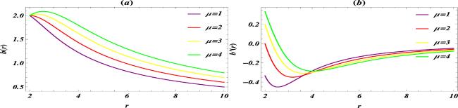
Figure 1. The left plots (a) reveal the behavior of b(r) while the right plots (b) show the behavior of $b^{\prime} (r)$ against r for a CCWH between two parallel plates. Herein, we set r0 = 2, Q = 0.25 and ε0 = 1. |
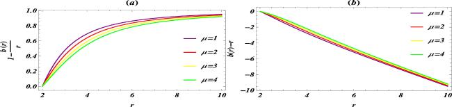
Figure 2. The left plots (a) reveal the behavior of 1 − b(r)/r while the right plots (b) show the behavior of b(r) − r against r for a CCWH between two parallel plates. |
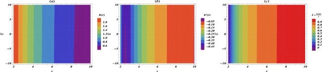
Figure 3. Contour plots illustrating b(r), $b^{\prime} (r)$ and 1 − b(r)/r with respect to radial coordinate r are presented in (a), (b) and (c), respectively, for a CCWH situated between two parallel plates when μ = 1. |

Figure 4. Contour plots depicting the NEC for a CCWH situated between two parallel plates. |
3.2. Case B: Casimir WH with charge induced by parallel cylinders
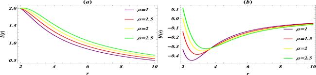
Figure 5. The left plots (a) reveal the behavior of b(r) while the right plots (b) reveal the behavior of $b^{\prime} (r)$ against r for a CCWH with energy density between the two parallel cylinders. Herein we set r1 = 0.1. |
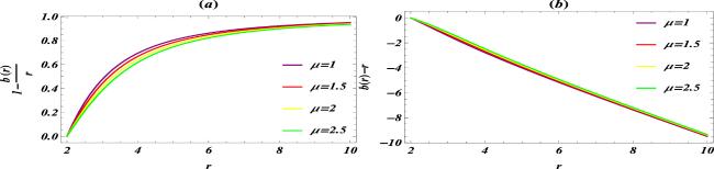
Figure 6. The left plots (a) reveal the behavior of 1 − b(r)/r while right plots (b) reveal the behavior of b(r) − r against r for a CCWH with energy density between the two parallel cylinders. |

Figure 7. Contour plots illustrating b(r), $b^{\prime} (r)$ and 1 − b(r)/r in terms of the radial coordinate r are presented in plots (a), (b) and (c), respectively, for a CCWH for the two parallel cylinders when μ = 1. |
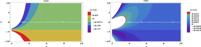
Figure 8. Contour plots illustrating the NEC for a CCWH positioned between two parallel cylinders. |
3.3. Case C: Casimir WH with charge induced by two spheres

Figure 9. The left plots (a) reveal the behavior of b(r) while the right plots (b) display the behavior of $b^{\prime} (r)$ against r for a CCWH for the case of two spheres. Herein we set A = 0.1. |
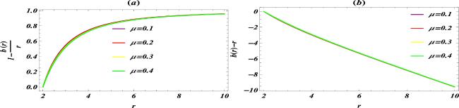
Figure 10. The left plots (a) reveal the behavior of 1 − b(r)/r while the right plots (b) reveal the behavior of b(r) − r against r for a CCWH for the case of two spheres. |

Figure 11. Contour plots illustrating b(r), $b^{\prime} (r)$, and 1 − b(r)/r in terms of the radial coordinate r are presented in plots (a), (b), and (c), respectively, for CCWH for the case of the two spheres when μ = 1. |

Figure 12. Contour plots showcasing the NEC for a CCWH situated between two parallel cylinders. |
3.4. Case D: charged Casimir GUP-corrected WH
| The behavior of b(r) can be seen from figure 13(a). Near the WH throat it is an increasing function of r, while it decreases away from the throat. Figure 13(b) shows that $b^{\prime} (r)\lt 1$, and it can be analyzed that for larger values of μ this condition is not satisfied. Figure 14(a) is plotted for the AF condition which says that $1-\displaystyle \frac{b(r)}{r}\to 1$ as r → ∞ and μ = 10. For higher values of μ, the SF is no longer asymptotically flat. Moreover, the AF condition is also not satisfied for μ < 0. Figure (14)(b) depicts the throat point. | |
| The plot in figure 15(a) shows that charged GUP-corrected b(r) is a decaying function of Q when μ = 10. Figure 15(b) shows that for Q > 0, Q < 0 and Q = 0, $b^{\prime} (r)\lt 1$. In figure 15 (c) we can see that for Q > 0, Q < 0 and Q = 0 the AF condition is satisfied. | |
| Figure 16 shows contour plots of the NEC for a CCWH with GUP correction, specifically for the parameter ζ1. We can see that the NEC is not valid as ρ + pr ≥ 0 for μ ≤ −4 while ρ + pt ≥ 0 for μ ≥ −4. ρ is negative, therefore, NEC and WEC are not satisfied. This suggests the existence of exotic matter and the presence of a WH. The ranges of parameters are ρ > 0 for α < 0, Q > 0, ρ + pr > 0 for Q > 0 & μ < −5, ρ + pr > 0 for Q > 0 & 1 < μ < 2. In short, we could not find a common region for which conditions could hold, therefore, both the NEC and WEC are not satisfied. |

Figure 13. The left plots (a) reveal the behavior of b(r) while the right plots (b) reveal the behavior of $b^{\prime} (r)$ against r for a charged GUP-corrected WH for ζ1. Herein we set α = 2 and Q = 0.5. |
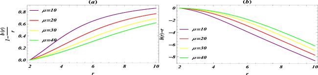
Figure 14. The left plots (a) reveals the behavior of 1 − b(r)/r while the right plots (b) reveal the behavior of b(r) − r against r for a charged GUP-corrected WH for ζ1. |
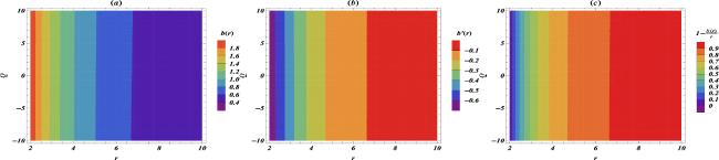
Figure 15. Contour plots illustrating b(r), $b^{\prime} (r)$ and 1 − b(r)/r in terms of the radial coordinate r are presented in plots (a), (b) and (c), respectively, for a charged GUP-corrected WH for ζ1 when μ = 10. |

Figure 16. Contour plots illustrating the NEC for a CCWH with GUP corrections, specifically for the parameter ζ1. |
4. Active gravitational mass in a CCWH
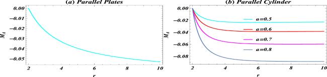
Figure 17. The left plot (a) shows ${M}_{{ \mathcal A }}$ of a WH from parallel plates while the right plots (b) show ${M}_{{ \mathcal A }}$ of a WH from parallel cylinders. Herein we set r0 = 2, ε0 = 0.5 and Q = 0.5. |
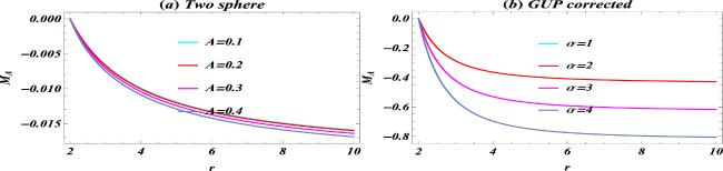
Figure 18. The left plots (a) display ${M}_{{ \mathcal A }}$ of a WH from two spheres while the right plots (b) show ${M}_{{ \mathcal A }}$ of a WH from GUP correction. |
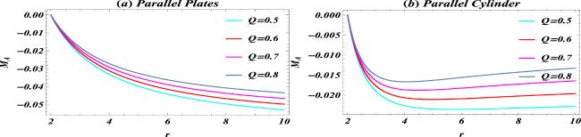
Figure 19. The left plots (a) display ${M}_{{ \mathcal A }}$ of a WH from parallel plates while the right plots (b) shows ${M}_{{ \mathcal A }}$ of a WH from parallel cylinders. The value of other parameters is a=0.5. |
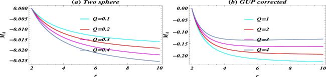
Figure 20. The left plots (a) display ${M}_{{ \mathcal A }}$ of a WH from two spheres while the right plots (b) show ${M}_{{ \mathcal A }}$ of a WH from the GUP-corrected energy density. The selected values of parameters are A = 0.1 and α = 1. |
5. Embedding diagram of charged Casimir WHs

Figure 21. 2D visualization of z(r) for a CCWH for cases A (left) and B (right). |
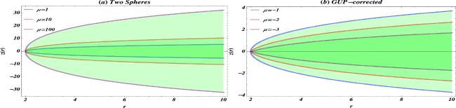
Figure 22. 2D visualization of z(r) for a CCWH for cases C (left) and D (right). |
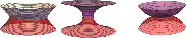
Figure 23. The dynamics of entire surface visualization for a CCWH are produced by rotating the embedded curve about the vertical z axis. Here μ = 100. |
6. Behavior of the CF on charged Casimir WHs

Figure 24. The left plot (a) reveals the CF of a CCWH induced between two parallel plates while the right plots (b) show the CF of a CCWH induced between two parallel cylinders. |
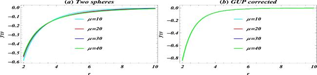
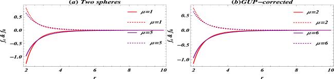
Figure 25. The left plots (a) reveal the CF of a CCWH induced between two spheres while the right plots (b) show the CF of a charged GUP-corrected WH. |
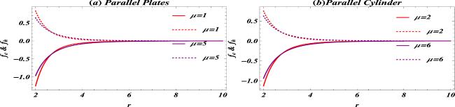
Figure 26. The left plots (a) reveal the equilibrium configuration of a CCWH due to two parallel plates while the right plots (b) display the equilibrium configuration of a CCWH due to two parallel cylinders. The values of the other parameters are Q = 0.25, a = 1 and ε0 = 1. |
7. Equilibrium forces for a charged Casimir WH
Figure 27. The left plots (a) reveal the equilibrium configuration of a CCWH due to two spheres while the right plots (b) display the equilibrium configuration of a charged GUP-corrected Casimir WH. The values of the other parameters are Q = 0.25, A = 0.1 and ε0 = 1. |
8. Summary
| We assumed energy densities between parallel plates, cylinders and spheres and due to the GUP-corrected function. To find out the SF we compared the energy density of EGB gravity and that due to the charged Casimir source. Ultimately, we graphically examined the b(r) derived for each system. We noticed that under the asymptotic background, the b(r) we obtained meet the flare-out criterion. Also, we observed how modified gravity impacted the SF. In the scenario of a GUP-corrected WH, we used the KMM model, as the behavior of the KMM and DGS models is similar. All the WH conditions were evaluated through 2D plots. Moreover, we plotted contour plots by varying the electric charge parameter and fixing the GB-coupled parameters. We also observed that b(r) grows with growth in the value of the GB-coupled parameter in each case, but b(r) is a declining function of electric charge. It was also found that $b^{\prime} (r)\lt 1$ for μ < 0, μ > 0, μ = 0. This condition is also satisfied for Q > 0, Q < 0 and Q = 0. The AF condition is not violated for μ > 0 only. However, when μ is fixed, it is satisfied for Q > 0, Q < 0 and Q = 0. | |||||||||||||||||||||||||||||||||||
| The NEC and WEC at the WH throat and far away from the throat were also explored. It was observed that the WEC in each case is violated due to the presence of negative Casimir energy density. | |||||||||||||||||||||||||||||||||||
| We also studied ${M}_{{ \mathcal A }}$ of a WH, which was developed in this article. The Casimir effect currently acts as a visible manifestation of such exotic matter. The presence of a negative ${M}_{{ \mathcal A }}$ shows the existence of exotic matter. When measured in a particular area of space, the Casimir effect produces a negative value for ${M}_{{ \mathcal A }}$. We studied the behavior of the ${M}_{{ \mathcal A }}$ of a WH in each case for a constant value of Q, where we observed that ${M}_{{ \mathcal A }}$ is negative for each case. In all cases, ${M}_{{ \mathcal A }}$ decreases with increasing value of a, A and α. Further, we saw that when the electric charge increases, ${M}_{{ \mathcal A }}$ increases. However, ${M}_{{ \mathcal A }}$ decreases for the WH model developed from two concentric spheres with an increase in electric charge. For the GUP-corrected WH, ${M}_{{ \mathcal A }}$ decays with increase in Q. | |||||||||||||||||||||||||||||||||||
| Using mathematical models to characterize the developed WHs in both 3D and 2D spacetimes, we explored the geometry of WHs. The energy densities of these WHs are responsible for manifestation of charged Casimir phenomena. We noted that the SF b(r) satisfies every prerequisite for the existence of a WH. In order to illustrate the geometry of the WH for various CCWH scenarios, specifically when t is held constant and θ is set to $\tfrac{\pi }{2}$, we presented graphical representations in the form of embedded diagrams. In addition, we presented two asymptotically flat WHs displaying a cosmos in both 3D and 2D spacetimes. | |||||||||||||||||||||||||||||||||||
| We also studied the dynamics of the CF for each scenario in order to understand the system's complexity. Based on the values of μ and Q, we found that ${{ \mathcal Y }}_{{TF}}$ constantly falls within a particular range, namely $-1\lt {{ \mathcal Y }}_{{TF}}\leqslant 0$. ${{ \mathcal Y }}_{{TF}}$ tends to approach zero as we go away from the WH throat. The results in [43] show that a configuration with uniform energy density (ρ) and isotropic pressure has a null CF. In contrast, a CF can also be zero in the presence of an anisotropic pressure and an inhomogeneous energy density, provided that these two effects cancel each other out in the CF. In the present study, the CF exhibits a monotonic increase close to the WH throat while it slowly approaches zero for larger radial coordinates. | |||||||||||||||||||||||||||||||||||
| Equilibrium forces for a CCWH for each case have been calculated and plotted. We found that for r > 6 forces completely balance each other's effects. | |||||||||||||||||||||||||||||||||||
| Casimir WHs in the background of EGB gravity were explored for the first time without considering the effects of electric charge in [70]; Casimir energy density was considered (energy density due to induction of the GUP effect and developed SF). The WH conditions were assessed in simple 2D plots and in terms of contour plots to find the dynamics of μ. Contour plots were plotted to understand the behavior of GB-coupled parameters in specific domains. Moreover, to measure the deviation of EGB gravity from GR, the findings in [70] were compared with the results found in [51]. The present manuscript is designed to explore the Casimir energy densities with the inclusion of electric charge by utilizing the idea presented in [60]. We considered different energy densities, developed the SF and evaluated their properties. By taking the influence of electric charge into consideration, we obtained an asymptotically flat SF. The behavior of the GB-coupled parameter μ and electric charge parameter Q were studied in detail. We observed that the presence of Q has a strong influence on the behavior of the SF. Moreover, by substituting Q = 0 and ε0 = 1 in each result of the present article, we obtained the same outcomes as in [70]. Summary tables with all the findings are given below (tables 1 and 2).
| |||||||||||||||||||||||||||||||||||
| We also contrasted our findings with one from GR. We have two independent, maximally symmetric solutions for our acquired SF. Although it is possible for both solutions to exhibit different asymptotic behaviors GR does not exhibit this. The expression of the SF from GR is only dependent on radial distance r. In the case of EGB gravity, we have an additional parameter or degree of freedom to comprehend the dynamics. Similarly, EGB gravity has two degrees of freedom, μ and α, in the scenario of a CCWH with GUP correction. The effects of Casimir energy densities within different modified theories have also been studied by many authors [52, 55, 56, 58], where they inculcated the ideas of Garattini, which he presented in [51]. In the current article, we used a newly introduced concept of Garattini, an extension of his previous work [60], and studied four different systems of Casimir energy density. Consequently, this research delivers a new perspective on the subject of CCWHs studied in higher-dimensional gravities. |