


1. Introduction
In 1914, Nordström first proposed the concept of extra dimensions [1, 2]. In the 1920s, Klein and Kaluza introduced the extra dimension theory, also known as the Klein–Kaluza (KK) theory, to unify the four-dimensional electromagnetic and gravitational interactions [3, 4]. However, there was no noticeable development in the following decades. Until the establishment of quantum field theory, the gauge hierarchy problem (fine-tuning problem) appeared in the Standard Model. The simple description is why the Planck scale is about 16 orders of magnitude higher than the weak scale. In the 1990s, in order to solve the hierarchy problem, Arkani-Hamed, Dimopoulos, and Dvali (ADD) proposed the large extra-dimensional theory [5]. Then, Antoniadis, Arkani-Hamed, Dimopoulos, and Dvali first embed the braneworld model into string theory [6]. However, the ADD model only shifted the hierarchy problem to the scale of the extra dimension. In 1999, Randall and Sundrum (RS) proposed a warped extra-dimensional model, which successfully solved the hierarchy problem without the shortcomings of the ADD model [7]. In the same year, they proposed another extra-dimensional model that can realize the four-dimensional Newtonian potential on the brane even though the size of the extra dimension is infinite [8]. The thickness of the RS brane is infinitely thin. But can there be a thick brane with infinite one or more extra dimensions? Based on this idea, the thick brane theory was developed [9–11]. That is, the matter is localized on the brane by the effective potential generated by the space–time background. After that, various related extra-dimensional models were developed [9, 10, 12–30].
In thick brane models, it is expected that the zero modes of various fields will be localized on the brane. The localization mechanism of these fields on the brane has been well established in different gravitational theories [10, 11, 17, 31–51]. Since fundamental matters consist of fermions, the nature of spin 1/2 fermions is important in braneworld models. Typically, interactions with background fields are introduced to enable the localization of either left- or right-chiral fermion zero mode on the brane [40, 45–50]. Usually, the massive fermion KK modes are not localized on the brane. However, some of them may be quasi-localized on the brane. Such massive modes are known as fermion resonances. It is worth noting that the resonances are fundamentally a unique category of quasi-normal modes in the context of thick brane backgrounds, known as quasi-normal resonant modes [52–56]. Previous literature has investigated the resonances of various fields in thick brane models [45, 57–64]. But the evolution of these resonances has been rarely studied.
The detection of extra dimensions is one of the most exciting questions in physics. Various models of extra dimensions offer distinct experimental implications. For instance, in certain thick brane models, the presence of KK gravitons can induce modifications in the Newtonian gravitational potential [8, 22, 24, 31, 33, 39, 44, 60, 61, 63, 64]. Moreover, the detection of gravitational waves brings attention to the possibility of observing the short-cut effect of gravitational waves predicted in some extra-dimensional models, providing an additional way for detecting the presence of extra dimensions [65–67]. Recently, we have numerically studied the dynamic of the scalar resonance on a thick brane and showed that the lifetime of the scalar resonance can be long enough to reach the age of the Universe, which provides the possibility that the scalar resonances can be considered as a potential candidate for dark matter [68]. A natural question is whether there are sufficiently long-lived resonances on a thick brane for a high-dimensional Dirac field. While neutrinos are currently one of the most favored candidates for dark matter among fermions [69], it is worth noting that usual fermions, such as electrons and quarks, are more readily detectable due to their stronger interactions with the photon. Consequently, long-lived KK fermions, which arise in theories with extra dimensions, present an advantageous way for exploring the existence of these extra spatial dimensions. The extended lifetimes of these KK fermions facilitate their detection and can be employed as a characteristic mode for probing the presence of extra dimensions in experimental investigations. Thus, despite not being directly associated with dark matter, these long-lived KK fermions offer a possible way of verifying the existence of extra dimensions. Therefore, in this paper, we would like to investigate the dynamical evolution of fermion resonances in a thick brane model.
The remaining part of this paper is structured as follows. In section 2 , we introduce the localization mechanism of a five-dimensional Dirac fermion on a brane and derive the dynamical evolution equations of the Dirac field and the equations of motion of the left- and right-chiral fermion KK modes. In section 3 , we obtain the resonances of the five-dimensional fermion and derive their lifetimes in terms of the full width at half maximum. In section 4 , we obtain the half-life through the decay of energy by numerically solving the evolution equations. Finally, we give the discussions and conclusions in section 5 .
2. Five-dimensional Dirac field
First, we review the localization of a five-dimensional fermion on a brane [45, 47–50]. The mechanism is implemented by introducing a coupling between the background scalar field and the fermion field. In this paper, we consider the following action of a five-dimensional Dirac fermion with the Yukawa coupling [70–72]
$\begin{eqnarray}\begin{array}{l}{S}_{\tfrac{1}{2}}=\displaystyle \int {{\rm{d}}}^{5}x\sqrt{-g}\,\left[\bar{{\rm{\Psi }}}{{\rm{\Gamma }}}^{M}({\partial }_{M}+{\omega }_{M}){\rm{\Psi }}+\eta \bar{{\rm{\Psi }}}F(\phi ){\rm{\Psi }}\right],\end{array}\end{eqnarray}$
where F(φ) is the function of the background scalar field φ and η is the Yukawa coupling parameter. In five-dimensional spacetime, the Dirac field $\Psi$ is a four-component spinor. The spin connection ωM is given by $\begin{eqnarray}{\omega }_{M}=\displaystyle \frac{1}{4}{\omega }_{M}^{\bar{M}\bar{N}}{{\rm{\Gamma }}}_{\bar{M}}{{\rm{\Gamma }}}_{\bar{N}},\end{eqnarray}$
where $\begin{eqnarray}\begin{array}{rcl}{\omega }_{M}^{\bar{M}\bar{N}} & = & \displaystyle \frac{1}{2}{E}^{N\bar{M}}({\partial }_{M}{E}_{N}^{\bar{N}}-{\partial }_{N}{E}_{M}^{\bar{N}})\\ & & -\,\displaystyle \frac{1}{2}{E}^{N\bar{N}}({\partial }_{M}{E}_{N}^{\bar{M}}-{\partial }_{N}{E}_{M}^{\bar{M}})\\ & & -\,\displaystyle \frac{1}{2}{E}^{P\bar{M}}{E}^{Q\bar{N}}{E}_{M}^{\bar{R}}({\partial }_{P}{E}_{Q\bar{R}}-{\partial }_{Q}{E}_{P\bar{R}}).\end{array}\end{eqnarray}$
Here, capital Latin letters M, N,... = 0, 1, 2, 3, 5 label the five-dimensional spacetime indices, while letters $\bar{M},\bar{N},...\,=0,1,2,3,5$ label Lorentz ones. The Gamma matrices satisfy {ΓM, ΓN} = 2gMN and the vielbein ${E}_{\,\,\bar{M}}^{M}$ satisfies ${E}_{\,\,\bar{M}}^{M}{E}_{\,\,\bar{N}}^{N}{\eta }^{\bar{M}\bar{N}}={g}^{{MN}}$.We consider a static flat brane that satisfies four-dimensional Poincaré invariance on the brane, just as the scenario considered in the work of Randall and Sundrum [8]. This means that the induced metric at every point of the extra dimension is a four-dimensional flat metric, and the component of the five-dimensional metric is only related to the extra-dimensional coordinate y. The metric form that satisfies the above conditions is [7, 8, 43, 70, 73, 74]4 ) can be rewritten as5 ), the nonvanishing components of the spin connection (2 ) are ${\omega }_{\mu }=\tfrac{1}{2}{\partial }_{z}A{\gamma }_{\mu }{\gamma }_{5}$. The five-dimensional Dirac equation can be obtained by varying the action as follows7 ) into equation (6 ), we can rewrite equation (6 ) as9 ) can be rewritten as11 ), we finally derive the Schrödinger-like equations
$\begin{eqnarray}\begin{array}{rcl}{\rm{d}}{s}^{2} & = & {g}_{{MN}}{\rm{d}}{x}^{M}{\rm{d}}{x}^{N}\\ & = & {{\rm{e}}}^{2A(y)}{\eta }_{\mu \nu }{\rm{d}}{x}^{\mu }{\rm{d}}{x}^{\nu }+{\rm{d}}{y}^{2},\end{array}\end{eqnarray}$
where e2A(y) is the warp factor. With the coordinate transformation dy = eA(z)dz, the above metric ( $\begin{eqnarray}\begin{array}{l}{\rm{d}}{s}^{2}={{\rm{e}}}^{2A(z)}({\eta }_{\mu \nu }{\rm{d}}{x}^{\mu }{\rm{d}}{x}^{\nu }+{\rm{d}}{z}^{2}),\end{array}\end{eqnarray}$
which is very useful in the following discussion of the equations of motion for the Dirac field. Here, the Greek letter μ, ν = 0, 1, 2, 3 labels the four-dimensional spacetime indices. We assume that the warp factor e2A(y) and the scalar field φ(y) are only functions of the extra dimension coordinate y. From the conformal flat metric ( $\begin{eqnarray}\left[{\gamma }^{\mu }{\partial }_{\mu }+{\gamma }^{5}({\partial }_{z}+2{\partial }_{z}A)+\eta F\right]{\rm{\Psi }}=0.\end{eqnarray}$
Then we introduce the following chiral decomposition of the Dirac field: $\begin{eqnarray}\begin{array}{rcl}{\rm{\Psi }}({x}^{i},t,z) & = & {{\rm{e}}}^{-2A}{\rm{\Psi }}^{\prime} ({x}^{i},t,z)\\ & = & {{\rm{e}}}^{-2A}\displaystyle \sum _{n}\left[{\psi }_{{\rm{L}}n}({x}^{i}){F}_{{\rm{L}}n}(t,z)\right.\\ & & \left.+\,{\psi }_{{\rm{R}}n}({x}^{i}){F}_{{\rm{R}}n}(t,z)\right],\end{array}\end{eqnarray}$
where i = 1, 2, 3 label three-dimensional space indices, ψLn = − γ5ψLn and ψRn = γ5ψRn are left- and right-chiral three-dimensional space components of the Dirac field, respectively. Substituting the chiral decomposition ( $\begin{eqnarray}\left[{\gamma }^{\mu }{\partial }_{\mu }+{\gamma }^{5}{\partial }_{z}+\eta F\right]{\rm{\Psi }}^{\prime} =0,\end{eqnarray}$
or as the chiral form $\begin{eqnarray}\begin{array}{l}{\rm{i}}({\partial }_{t}+{\sigma }^{i}{\partial }_{i}){F}_{{\rm{R}}n}{\psi }_{{\rm{R}}n}=({\partial }_{z}+\eta F){F}_{{\rm{L}}n}{\psi }_{{\rm{L}}n},\\ {\rm{i}}({\partial }_{t}-{\sigma }^{i}{\partial }_{i}){F}_{{\rm{L}}n}{\psi }_{{\rm{L}}n}=(-{\partial }_{z}+\eta F){F}_{{\rm{R}}n}{\psi }_{{\rm{R}}n},\end{array}\end{eqnarray}$
where σi are the Pauli matrix. The above equations ( $\begin{eqnarray}\begin{array}{l}\left[{\partial }_{t}^{2}-{\partial }_{i}^{2}-{\partial }_{z}^{2}+{V}_{{\rm{L}}}(z)\right]{F}_{{\rm{L}}n}{\psi }_{{\rm{L}}n}=0,\\ \left[{\partial }_{t}^{2}-{\partial }_{i}^{2}-{\partial }_{z}^{2}+{V}_{{\rm{R}}}(z)\right]{F}_{{\rm{R}}n}{\psi }_{{\rm{R}}n}=0.\end{array}\end{eqnarray}$
We consider free modes on the brane, i.e., ${\psi }_{{\rm{L}}n,{\rm{R}}n}({x}^{i})={{\rm{e}}}^{-{\rm{i}}{a}_{{ni}}{x}^{i}}{\chi }_{{\rm{L}}n,{\rm{R}}n}$, where χLn,Rn are four-dimensional spinors independent of the coordinate and ani corresponds to the spatial momentum of the spinors on the brane. Then we can obtain the following evolution equations: $\begin{eqnarray}\begin{array}{l}\left[{\partial }_{t}^{2}-{\partial }_{z}^{2}+{V}_{{\rm{L}}}(z)\right]{F}_{{\rm{L}}n}=-{a}_{n}^{2}{F}_{{\rm{L}}n},\\ \left[{\partial }_{t}^{2}-{\partial }_{z}^{2}+{V}_{{\rm{R}}}(z)\right]{F}_{{\rm{R}}n}=-{a}_{n}^{2}{F}_{{\rm{R}}n},\end{array}\end{eqnarray}$
where ${a}_{n}=\sqrt{{a}_{{ni}}{a}_{n}^{i}}$ and the effective potentials VL,R are [43, 47, 72, 75–77] $\begin{eqnarray}{V}_{{\rm{L,R}}}{(z)=(\eta {e}^{A}F)}^{2}\pm {\partial }_{z}(\eta {e}^{A}F).\end{eqnarray}$
We further decompose FLn and FRn as $\begin{eqnarray}{F}_{{\rm{L}}n,{\rm{R}}n}(t,z)={{\rm{e}}}^{{\rm{i}}\omega t}{f}_{{\rm{L}}n,{\rm{R}}n}(z).\end{eqnarray}$
Substituting the above decompositions into equation ( $\begin{array}{l} {\left[-\partial_{z}^{2}+V_{\mathrm{L}}(z)\right] f_{L n}=m_{n}^{2} f_{\mathrm{L} n}} ,\\ {\left[-\partial_{z}^{2}+V_{\mathrm{R}}(z)\right] f_{R n}=m_{n}^{2} f_{\mathrm{R} n}}, \end{array}$
where mn is the mass of the corresponding Dirac KK modes.3. Fermion localization and resonance
In this section, we investigate the resonances of a bulk fermion and their evolution in the thick brane model. The action of the thick brane is [9–11, 47, 78–80]19 ) into equations (17 ) and (18 ), we can get the form of the scalar field and the warp factor under the conformal coordinate z:
$\begin{eqnarray}\begin{array}{l}S=\displaystyle \int {{\rm{d}}}^{5}x\sqrt{-g}\,\left[\displaystyle \frac{{M}_{5}^{3}}{4}R-\displaystyle \frac{1}{2}{\partial }_{M}\phi {\partial }^{M}\phi -V(\phi )\right].\end{array}\end{eqnarray}$
We set the fundamental mass scale M5 = 1 for convenience. A flat brane solution was studied in [11, 47, 50, 80] $\begin{eqnarray}V(\phi )=\displaystyle \frac{9}{8}{k}^{2}{b}^{2}{\cosh }^{2}(b\phi )-3{k}^{2}{\sinh }^{2}(b\phi ),\end{eqnarray}$
$\begin{eqnarray}\phi (y)=\displaystyle \frac{1}{b}\mathrm{arcsinh}\left[\tan \left(\displaystyle \frac{3}{2}{{kb}}^{2}y\right)\right],\end{eqnarray}$
$\begin{eqnarray}A(y)=-\displaystyle \frac{2}{3{b}^{2}}\mathrm{ln}\left[\sec \left(\displaystyle \frac{3}{2}{{kb}}^{2}y\right)\right],\end{eqnarray}$
where k, b are real parameters. In this paper, we choose $b=\sqrt{2/3}$. The conformal coordinate is $\begin{eqnarray}\begin{array}{l}z={\int }_{0}^{y}{{\rm{e}}}^{-A(y)}{\rm{d}}y=\displaystyle \frac{1}{k}\mathrm{arcsinh}\left[\tan ({ky})\right].\end{array}\end{eqnarray}$
Substituting the relation ( $\begin{eqnarray}\phi (z)=\sqrt{\displaystyle \frac{3}{2}}{kz},\end{eqnarray}$
$\begin{eqnarray}A(z)=\mathrm{ln}\left[{\rm{{\rm{sech}} }}({kz})\right].\end{eqnarray}$
To study the localization of a five-dimensional fermion on the thick brane, we consider the Yukawa coupling $\eta \bar{{\rm{\Psi }}}F(\phi ){\rm{\Psi }}$ between the fermion $\Psi$ and the background scalar field φ. The coupling function is chosen as $F(\phi )\,=k\,{\mathrm{arcsinh}}^{2q-1}(b\phi )$, where the structure parameter q is a positive integer [45]. By substituting the specific form of F(φ) into equation (12 ), we can obtain the expression of the effective potential:14 ). For simplicity, here we do not consider the impact of the change in k on the potential function and take k = 1.
$\begin{eqnarray}\begin{array}{rcl}{V}_{{\rm{L}},{\rm{R}}}(z) & = & \pm \eta \,{k}^{2}\,{\rm{sech}} \left({kz}\right){\mathrm{arcsinh}}^{2q-2}\left({kz}\right)\\ & & \times \left(\displaystyle \frac{(2q-1)}{\sqrt{1+{k}^{2}{z}^{2}}}\pm \eta \,{\mathrm{arcsinh}}^{2q}\left({kz}\right)\right.\\ & & \times \left.{\rm{{\rm{sech}} }}\left({kz}\right)-\mathrm{arcsinh}\left({kz}\right)\tanh \left({kz}\right)\right).\end{array}\end{eqnarray}$
We plot the effective potentials with different values of the coupling parameter η in figure 1. Note that we always have VL,R(0) = 0. It can be seen that the stronger the coupling, the deeper the (quasi) potential wells. In addition to the coupling parameter η, there are also two parameters k and q that affect the potential functions. We also give the plots of the potentials with different values of q in figure 2. Obviously, similar behaviors induced by the coupling parameter η are also found when changing the parameter q, i.e., the depth of the quasi potential well increases with q. Note that the parameter k only rescales the eigenvalues of Schrödinger-like equations (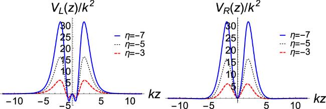
Figure 1. The shapes of the effective potentials ( |

Figure 2. Plots of the effective potentials and the relative probabilities for the left-chiral fermion for different values of q. |
The solutions of the left and right-chiral zero modes are
$\begin{eqnarray}\begin{array}{l}{f}_{{\rm{L}}0,{\rm{R}}0}\propto {{\rm{e}}}^{\pm \eta \int F(\phi ){\rm{d}}z}\\ \,=\,{{\rm{e}}}^{\pm \eta \int {\mathrm{arcsinh}}^{2q-1}(\phi ){\rm{d}}z}\mathop{\longrightarrow }\limits^{z\to \infty }{{\rm{e}}}^{\pm }\eta z{\left(\mathrm{ln}z\right)}^{2q-1}.\end{array}\end{eqnarray}$
It can be seen that, when the coupling η is negative, only the left-chiral zero mode satisfies $\begin{eqnarray}\begin{array}{l}{\displaystyle \int }_{-\infty }^{\infty }| {f}_{{\rm{L}}0}{| }^{2}{\rm{d}}z\lt \infty .\end{array}\end{eqnarray}$
Thus, only the left-chiral zero mode can be localized on the brane for a negative coupling [45, 47–50]. Conversely, only the right-chiral zero mode can be localized on the brane for a positive coupling.Next, we investigate the characteristics of fermion resonances for this braneworld model. Apart from the zero mode, there exist some massive KK modes that are quasi-localized on the brane, which are called resonances. In 2009, Almeida et al defined resonances by using the peak value of the square of a normalized wave function at a fixed point in the well of the effective potential [58]. Subsequently, the relative probability method was introduced to look for all resonances [57]. In 2011, the transfer matrix method was used to obtain resonances [81]. A resonance is a massive KK mode quasi-localized within an effective (quasi) potential well, i.e., quasi-localized on the brane. For a resonance, its transmitted and reflected oscillatory modes are in phase in the effective (quasi) potential well. A resonant state usually has a larger amplitude within the brane. Thus, one can employ the probability ratio of a massive KK mode inside the brane (−zb, zb) and inside a wider range of extra dimension $(-{z}_{\max },{z}_{\max })$ to quantify the reflectivity in a relatively straightforward manner, without the need for a transfer matrix approach. Specifically, we consider the range of extra dimension to be n times of the brane, i.e., ${z}_{\max }={{nz}}_{b}$. For a plane wave mode, the probability ratio is 1/n. If the probability ratio exceeds 1/n, the reflection will exceed the transmittance and the massive mode might be a resonance. In this paper, we use the relative probability method to find all resonances. The relative probability is defined as [57]
$\begin{eqnarray}\begin{array}{l}{P}_{{\rm{L,R}}}({m}^{2})=\displaystyle \frac{{\displaystyle \int }_{-{z}_{b}}^{{z}_{b}}| {f}_{{\rm{L}}n,{\rm{R}}n}(z){| }^{2}{\rm{d}}z}{{\displaystyle \int }_{-{z}_{\max }}^{{z}_{\max }}| {f}_{{\rm{L}}n,{\rm{R}}n}(z){| }^{2}{\rm{d}}z},\end{array}\end{eqnarray}$
where ${z}_{\max }={{nz}}_{b}$ and zb is approximately the width of the brane. Each local maximum of the relative probability with a full width at half maximum corresponds to a resonance. We focus on the dynamic behavior of the resonances in the brane, so zb is taken as the coordinate value corresponding to the maximum of the potential. If the range of extra dimension is too small, the relative probability error will be large. For a not too small ${z}_{\max }$, e.g., ${z}_{\max }\geqslant 10{z}_{b}$, its value has no effect on the resonance spectrum. Here, we take n = 10. Since the effective potential is symmetric, we can take the following boundary conditions to obtain the massive KK modes numerically: $\begin{eqnarray}{f}_{{\rm{L}}n,{\rm{R}}n}(0)=0,\,f{{\prime} }_{{\rm{L}}n,{\rm{R}}n}(0)=1,\,\mathrm{odd}\ \mathrm{KK}\ \mathrm{modes},\end{eqnarray}$
$\begin{eqnarray}{f}_{{\rm{L}}n,{\rm{R}}n}(0)=1,\,f{{\prime} }_{{\rm{L}}n,{\rm{R}}n}(0)=0,\,\mathrm{even}\ \mathrm{KK}\ \mathrm{modes}.\end{eqnarray}$
For a KK mode with the mass mn, if its relative probability P(m2) has just a peak at m = mn and this peak has a full width at half maximum, we say that there is a resonance with the mass mn. The relative probabilities of a left-chiral fermion's massive mode for different q are shown in figure 2. It shows that the depth and width of the quasi-well significantly increase with the parameter q. It means that the number and the relative probabilities of resonances also increase greatly with q. The relative probabilities of the massive KK modes of the left- and right-chiral fermions for different η are shown in figure 3. It is evident that the peak value and the number of resonances increase with ∣η∣. Since the resonance cannot be localized on the brane, it can only stay on the brane for a finite time. Here, we use the full width at half maximum to roughly estimate the lifetime of the resonances. Usually, the first resonance has the longest lifetime. It should be noted that, in other thick brane models, the first resonance may not be the longest-lived mode [48, 82]. In our model, we can see that the relative probability of the resonance decreases with the mass mn, correspondingly, the lifetime of the resonance also decreases with the mass mn. We can also see that the left- and right-chiral fermions share the same resonant spectrum. The reason is that the finite effective potentials (12 ) of the left- and right-chiral fermions are supersymmetric partner potentials, and there are finite in the whole region. So they have exactly the same mass spectrum except for the zero mode, which was also discussed in [43, 45, 47, 76, 77]. Therefore, even though the right-chiral fermion lacks a zero mode and cannot be fully localized on the brane for negative coupling parameter η, some long-lived modes can be quasi-localized on the brane, which enables the possibility of detecting right-chiral fermions. The wave functions of the resonances and nonresonances for the case of η = –7 and q = 2 are shown in figure 4. It can be seen that, for a resonance, the amplitude of its wave function inside the potential well is much larger than that outside the well. The opposite is true for nonresonances. So far, we have introduced the relative probability method to derive the resonances. Next, we will focus on the evolution of them.
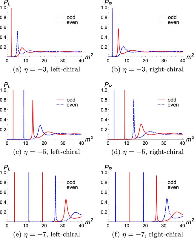
Figure 3. Plots of the relative probabilities of the left- and right-chiral fermion KK modes for different values of η and fixed value q = 2. The red lines are odd-parity modes and the blue dashed lines are even-parity modes. |
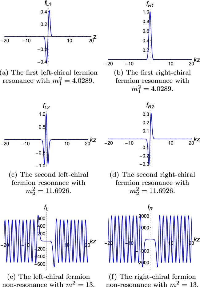
Figure 4. Plots of the wave functions of different chiral resonances. |
4. Resonance evolution
In this section, we investigate the evolution behavior of fermion resonances. Under the stationary assumption, one can obtain such resonances in terms of the relative probability. Since these resonances are not localized on the brane, they cannot exist stably on it. Therefore, one can take them as the initial data and numerically evolve them by using equation (11 ) with the radiation boundary condition [83].
Note that, a resonance cannot be localized on the brane and the corresponding total energy is divergent. Such divergent total energy means that one cannot use it to grasp the dynamical properties of the resonance. To overcome this disadvantage, we define an effective energy of the resonance in a finite range (−zb, zb) in terms of the energy-momentum tensor. The specific form of the energy-momentum tensor TMN in the case of the action (1 ) in five-dimensional spacetime is28 ) into the above equation, we can get
$\begin{eqnarray}\begin{array}{rcl}{T}_{{MN}} & = & \displaystyle \frac{1}{2}(\bar{{\rm{\Psi }}}{{\rm{\Gamma }}}_{M}({\partial }_{N}+{\omega }_{N}){\rm{\Psi }}+\bar{{\rm{\Psi }}}{{\rm{\Gamma }}}_{N}({\partial }_{M}+{\omega }_{M}){\rm{\Psi }})\\ & & +\,{g}_{{MN}}\left(\bar{{\rm{\Psi }}}{{\rm{\Gamma }}}^{K}({\partial }_{K}+{\omega }_{K}){\rm{\Psi }}+\eta \bar{{\rm{\Psi }}}F(\phi ){\rm{\Psi }}\right).\end{array}\end{eqnarray}$
Combining the energy-momentum tensor TMN and the time-like killing vector kN, one can derive the conserved current as [84] $\begin{eqnarray}{J}_{M}={T}_{{MN}}{k}^{N}.\end{eqnarray}$
Then we can define the corresponding energy [84]: $\begin{eqnarray}E(t)=\int {J}^{0}\sqrt{-g}{{\rm{d}}}^{3}x{\rm{d}}z.\end{eqnarray}$
Substituting equation ( $\begin{eqnarray}\begin{array}{rcl}E(t) & = & \displaystyle \int {\psi }_{{\rm{L}}}^{* }{\psi }_{{\rm{L}}}{{\rm{d}}}^{3}x{\displaystyle \int }_{-{z}_{b}}^{{z}_{b}}(2{\rm{i}}{F}_{{\rm{L}}}^{* }{\partial }_{t}{F}_{{\rm{L}}}-{a}_{n}{F}_{{\rm{L}}}^{* }{F}_{{\rm{L}}}){{\rm{e}}}^{A}{\rm{d}}z\\ & & +\,\displaystyle \int {\psi }_{{\rm{R}}}^{* }{\psi }_{{\rm{R}}}{{\rm{d}}}^{3}x{\displaystyle \int }_{-{z}_{b}}^{{z}_{b}}(2{\rm{i}}{F}_{{\rm{R}}}^{* }{\partial }_{t}{F}_{{\rm{R}}}+{a}_{n}{F}_{{\rm{R}}}^{* }{F}_{{\rm{R}}}){{\rm{e}}}^{A}{\rm{d}}z.\end{array}\end{eqnarray}$
In this paper, we focus on the evolution of fermion resonances along the extra dimension. Therefore, we only calculate the evolution of the extra dimension profile for the left- and right-chiral fermion KK modes separately. So the conserved energy simplifies to
$\begin{eqnarray}E(t)={ \mathcal B }{E}_{e}(t)={ \mathcal B }{\int }_{-{z}_{b}}^{{z}_{b}}\rho (t,z){{\rm{e}}}^{A}{\rm{d}}z,\end{eqnarray}$
where $\begin{eqnarray}{ \mathcal B }=\int {\psi }_{{\rm{L}},{\rm{R}}}^{* }{\psi }_{{\rm{L,R}}}{{\rm{d}}}^{3}x,\end{eqnarray}$
$\begin{eqnarray}{E}_{e}(t)={\int }_{-{z}_{b}}^{{z}_{b}}{\rho }_{{\rm{L}},{\rm{R}}}(t,z){{\rm{e}}}^{A}{\rm{d}}z,\end{eqnarray}$
$\begin{eqnarray}{\rho }_{{\rm{L}},{\rm{R}}}(t,z)=2{\rm{i}}{F}_{{\rm{L}},{\rm{R}}}^{* }{\partial }_{t}{F}_{{\rm{L}},{\rm{R}}}\mp {a}_{n}{F}_{{\rm{L}},{\rm{R}}}^{* }{F}_{{\rm{L}},{\rm{R}}}.\end{eqnarray}$
First, we consider the case of an = 0. The evolution of energy Ee(t) for each KK fermion is shown in figure 5. It can be seen that the first resonance with the smallest mass has the smallest decay rate. The decay rate of the resonance decreases with the parameter ∣η∣. We can also fit the decay of the energy Ee with the exponential form as follows
$\begin{eqnarray}{E}_{e}(t)={E}_{0}{{\rm{e}}}^{-{st}},\end{eqnarray}$
where s is the decay parameter. We define the lifetime τ by Ee(τ)/Ee(0) = 1/2. Thus, the relation between the lifetime and the decay parameter is $\tau =\tfrac{\mathrm{ln}2}{s}$. Note that the term ‘decay' solely refers to the energy loss of the fermion resonances on the brane over time. It does not involve any decay channel and decay product in particle physics.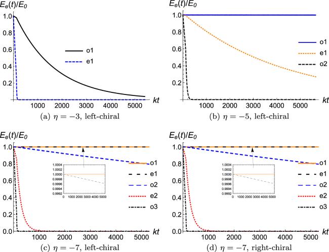
Figure 5. Plots of the energy as the function of time with different η and chirality. Parameter q set to 2. Here oj and ej represent the jth odd-parity and even-parity resonances, respectively. |
To investigate the dynamical behavior of a Dirac resonance, we can extract a time series for the amplitude of the resonance at a fixed point zext. The parameters are set to η = –7 and q = 2. We consider that there is no incident wave at infinity and the outgoing wave has no reflection behavior at boundaries at infinity. Therefore, we take the radiation boundary conditions at infinity on both sides: ∂tFL,R = ± ∂zFL,R for z → ± ∞ . The results are shown in figure 6, which reveals that the decay of the first resonance is the slowest. This phenomenon can be attributed to the fact that the mode with higher relative probability has a smaller amplitude outside the quasi-well than that inside the quasi-well. The reason is that the frequency of a resonance has a minimum transmittance. The greater the relative probability, the lower the transmittance and the slower the internal amplitude attenuation. For the boundary condition with outgoing waves on both sides, the rate of outflow of the reduced energy Ee(t)/E0 depends on both the difference between the internal and external amplitudes and the speed of outward movement. Thus, the greater the relative probability, the greater the difference between the internal and external amplitudes, and the slower the internal reduced energy decay. We present the results in table 1. It can also be seen that the lifetime calculated by using the full width at half maximum is much smaller than that obtained by evolution, and the greater the lifetime, the greater the error between the two ways, which can be also seen in figure 7. Therefore, the full width at half maximum can only be used to calculate the variation trend of the lifetime of the resonance very roughly, and cannot get the accurate lifetime value of a resonance.
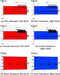
Figure 6. Time evolution of the amplitudes for the left- or right-chiral Dirac resonances at kzext = 2. The parameters are set to η = − 7 and q = 2. |
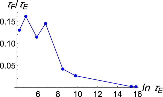
Figure 7. Plot of the relation between τF/τE and $\mathrm{ln}{\tau }_{E}$. τF and τE are the lifetimes calculated by the full width at half maximum and evolution, respectively. |
Table 1. The mass spectra m2n and mn, relative probability P, and lifetime τ of the left- and right-chiral KK fermion resonances for the Yukawa coupling. τFWHM and τNumerical are calculated by the full width at half maximum and evolution, respectively. The parameter is set to be q = 2. The symbols L and R are short for left-chiral and right-chiral, respectively. |
| η | parity | ${m}_{n}^{2}/{k}^{2}$ | mn/k | PL,R | kτFWHM | kτNumerical |
|---|---|---|---|---|---|---|
| odd | 2.2334 | 1.4945 | 0.9834 | 124.5 | 859.8 | |
| −3 | even | 5.5406 | 2.3654 | 0.5160 | 8.01 | 61.70 |
| | ||||||
| odd | 3.2301 | 1.7973 | 0.9996 | 8398.4 | 4.809 × 10⁶ | |
| −5 | even | 9.0202 | 3.0033 | 0.9944 | 202.3 | 4864 |
| odd | 13.8446 | 3.7236 | 0.7899 | 19.07 | 118.4 | |
| | ||||||
| odd | 4.0289 | 2.0072 | 0.9999 | 6.677 × 10⁶ | 1.997 × 10¹² | |
| even | 11.6926 | 3.4195 | 0.9998 | 1.005 × 10⁴ | 7.668 × 10⁶ | |
| −7 | odd | 19.0650 | 4.3664 | 0.9979 | 464.5 | 1.758 × 10⁴ |
| even | 26.0595 | 5.1059 | 0.9296 | 40.35 | 353.8 | |
| odd | 31.7044 | 5.6307 | 0.4553 | 6.306 | 78.20 | |
On the other hand, we can also treat a nonresonance as the initial data to perform its evolution. Figure 8 shows the evolution of the energy and the wave function for the nonresonance. As expected, the amplitude and the energy of the nonresonance quickly decay at an early stage, but later they decay like those of resonances. To gain a better understanding of this phenomenon, we perform the discrete Fourier transform and present the results in figure 9. The expression for the discrete Fourier transform is
$\begin{eqnarray}\begin{array}{l}F\left[{f}_{{\rm{L}}}(f,{z}_{\mathrm{ext}})\right]=| A\displaystyle \sum _{p}{f}_{{\rm{L}}}({t}_{p},{z}_{\mathrm{ext}})\,{{\rm{e}}}^{-2\pi {\rm{i}}{{ft}}_{p}}| ,\end{array}\end{eqnarray}$
where $A=1/\max (F\left[{f}_{{\rm{L}}}(f,{z}_{\mathrm{ext}})\right])$ is a normalized constant, and zext is a fixed point.
Figure 8. Time evolution of the reduced energy and the amplitude at kzext = 2 for the left-chiral Dirac KK modes with m2=13, η = − 7 and q = 2. |
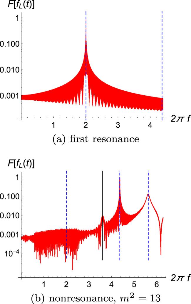
Figure 9. The Fourier transform spectrum of the amplitude at kzext = 2. The parameters are set to η = − 7 and q = 2. The dashed blue lines correspond to the frequencies of the three odd-parity resonances and the black line corresponds to the initial frequency. |
It is obvious that for the Fourier transform spectrum of the resonance, there is only one peak, which corresponds to the KK mass of the resonance. However, for the spectrum of the nonresonance, there are several peaks. Each peak corresponds to a resonance. This indicates that the nonresonance can evolve into a superposition of a series of resonances at late time.
In addition, we investigate the influence of the parameter η on the lifetime of the Dirac resonances. Since the energy decay rate of the first resonance state becomes extremely small when η is large, the accuracy error of calculation may be relatively large. Therefore, we choose the lifetime of the second resonance state here to study the relationship between its lifetime and the parameter η. The results are shown in table 2. It can be seen that the lifetime of the resonance increases with ∣η∣. This relationship can be attributed to the fact that the effective potential's height increases with ∣η∣, thereby elevating the relative probabilities of the resonances. Since the parameter η is the coupling strength of the background scalar field and the fermion, we can conclude that the stronger the coupling strength, the longer the lifetime of the fermion resonance on the brane.
Table 2. The lifetime τ of the second resonance. |
| η | −3 | −3.5 | −4 | −4.5 | −5 | −5.5 | −6 | −6.5 | −7 |
|---|---|---|---|---|---|---|---|---|---|
| kτ | 61.70 | 107.8 | 312.1 | 749.7 | 4864 | 1.940 × 10⁴ | 1.363 × 10⁵ | 7.982 × 10⁵ | 7.668 × 10⁶ |
In the previous part, we only consider the case of ani = 0, i.e, the momentum on the brane is zero. Next we consider the case of nonvanishing ani. According to equation (11 ), we can give the approximate form of the wave function at infinity:
$\begin{eqnarray}\begin{array}{l}{F}_{{\rm{L}}n,{\rm{R}}n}(t,z)\sim {{\rm{e}}}^{{\rm{i}}{\omega }_{n}(t-\tfrac{{m}_{n}}{{\omega }_{n}}z)}.\end{array}\end{eqnarray}$
So the wave speed is $v=\tfrac{{m}_{n}}{{\omega }_{n}}=\tfrac{{m}_{n}}{\sqrt{{m}_{n}^{2}+{a}_{n}^{2}}}$, where the dispersion relation is ${\omega }_{n}^{2}={m}_{n}^{2}+{a}_{n}^{2}$. It can be seen that the value of an and mn determines the velocity of the wave moving outward along the extra dimension at infinity. If an > 0, these KK particles travel along the extra dimension at a speed slower than light speed at extra-dimensional infinity.We plot the relation between the lifetime of the resonance and the parameter an in figure 10. The plot shows that the lifetime of the resonance increases with the parameter an, indicating that when the four-dimensional effective mass mn of the KK mode is a constant, the momentum of the KK mode has a positive correlation with its lifetime. Specifically, as an becomes sufficiently large, the lifetime of the resonance increases approximately linearly with an. Thus, when the momentum on the brane or the parameter q is much larger than 1 or the coupling is strong enough, the lifetime of the fermion resonance can be extremely long, possibly even lasting until the age of the Universe. For example, when the five-dimensional fundamental mass M5 is 10 TeV and the parameters are set to η = –7, q = 2, and an = 0, the lifetime of the first resonance state is about 40 million years. This suggests that it could offer the possibility of a new class of detectable fermion KK modes with different masses.
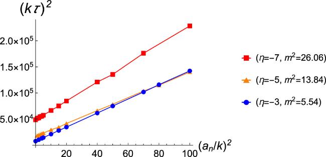
Figure 10. The relation between the lifetime of the resonance and an2 with q = 2. |
5. Conclusion
In this work, we investigated the evolution of Dirac KK modes in the thick brane. Starting from the brane solution given in [80], we obtained the evolution equations (11 ) and Schrödinger-like equations (14 ). Based on these equations, we obtained the solution of the resonances and studied their evolution. We found that the lifetime of these Dirac resonances can be very long. The resonance is a kind of important and interesting object in the braneworld. However, the dynamical behavior of Dirac resonances in the braneworld model has not been fully investigated. Thus, we still lack a comprehensive and profound understanding of the nature of the Dirac KK mode in braneworld model.
The fermion resonances were derived with the relative probability method established in [57]. We found that the number of resonances and the relative probability of the first resonance increase with the absolute value of the coupling parameter ∣η∣ and the parameter q, which can be seen from figures 2, 4, and table 2. Such behavior is similar to the previous literature [45, 48, 57, 58]. We also observed that a larger relative probability corresponds to a longer lifetime of the resonance, which is confirmed by the evolution of the KK mode presented in figures 5 and 6. Additionally, we investigated the evolution of the nonresonance. We found that its amplitude and energy decay promptly at the beginning. However, the later damping occurs in a similar manner as the resonances. Our results suggest that the nonresonance evolves into a superposition of the resonances, as demonstrated in figure 9. Furthermore, we obtained that the lifetime of a resonance almost linearly increases with the value of the three-dimensional momentum an, as shown in figure 10. If the parameter an, q, or ∣η∣ is large enough, the resonance may have a very long lifetime on the brane. It could offer the possibility of a new class of detectable fermions with different masses. At the same time, the measurement of the fermion mass can also limit the parameters in the model.
Next, it would be worthwhile to investigate whether a similar technique could be applied to the gravitational perturbation in extra-dimensional theory, potentially identifying it as a dark matter candidate. The effective potential in such theories typically has multiple potential barriers, which could allow for the study of the gravitational echo phenomenon in extra dimensions, analogous to that in black hole theory.
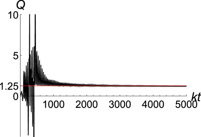
Appendix A. Convergence test
In the appendix, we will briefly discuss the convergence of our simulations, for which we compare the energy by using three space steps h = 1/32, 1/40, 1/50. This energy belongs to the first resonance with η = − 3.
In general, the numerical solutions of a system converge according to the following rule
$\begin{eqnarray}{\phi }_{h}-\phi \propto {h}^{n},\end{eqnarray}$
where h is the space step and n is the convergence order. We use the convergence factor Q to study its convergence behavior. Its form is $\begin{eqnarray}Q=\displaystyle \frac{{\phi }_{1}-{\phi }_{2}}{{\phi }_{2}-{\phi }_{3}}=\displaystyle \frac{{h}_{1}^{n}-{h}_{2}^{n}}{{h}_{2}^{n}-{h}_{3}^{n}}.\end{eqnarray}$
We give the corresponding results in figures 11 and 12. Using these results and the relation (A.2 ), we plot the convergence factor Q as a function of time in figure 12. We can see that Q ≃ 1.25, such value of Q means that the convergence order is of about 1. It can also be seen from figure 11 that as the space step size decreases, the energy error of the asynchronous step also decreases.
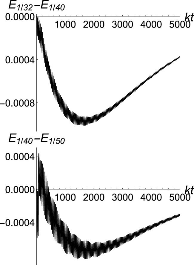
Figure 11. Plot of the energies error with different spatial step h. |
Figure 12. Plot of the evolution of the convergence factor Q. |