


Symmetry and topology are fundamental concepts penetrating into the core of different branches of physics. They are also tools that bridge seemingly different subjects into the same one. In this vein, an exemplification is the topologically protected edge waves due to the bulk-edge correspondence in condense matter materials [1]. Its counterpart in atmospheres and oceans is found to be the well-known Yanai and Kelvin waves [2]. Inspired by the celebrated Chern's number associated with Berry's phase in quantum system [3, 4], in this work, we report a topological number associated with the Kelvin's circulation (KC) in inviscid fluids—the Kelvin's number. Note that the quantization of the circulation in quantum fluids has been known for a long time [5–7].
A topological invariant refers to an integral that remains unchanged under continuous deformation of their integral domains [8]. When appropriately normalized, it appears as an integer, i.e., the topological number. A topological invariant is distinguished by its robustness against perturbations, as it always appears in a ‘quantized' manner, enabling it to tolerate continuous perturbations. Fundamentally, this feature reflects the robustness of the topological symmetry, which is the underlying symmetry associated with the conserved topological number [9].
In fluid dynamics, the best known–if not the only–topological invariant is the flow helicity and it is the number of the knots among vortex tubes [10]. Its generalizations include the magnetic helicity, the knots among magnetic field lines, and cross helicity, the linkage between vortex line and magnetic field line in magneto-fluids. The flow helicity has a general form as H = 2πmH1 with m the number of the knots and H1 a unit helicity [11]. It is inherently a 3D quantity, since one can only tie a knot in 3D space. The crucial constraint of the helicity conservation on turbulence relaxation has been studied, extensively [12]. Here, an interesting enquiry is: besides the knot, does there exist a topological number in 2D fluid dynamics or more generally independent of the spatial dimension?
In this work, we will show that the KC is related to such a topological invariant in 2D. To glimpse it, we start with the most essential meaning of a topological invariant—the multi-valuedness, which is generally linked with the integral of the geometric phase of a certain physical quantity [3]. A well studied subject in this field is the Berry's phase in quantum systems, which represents the variation of the geometric component of the wave function's phase along a closed parametric loop [4], and it has a form of loop integral:1 ) becomes:4 ) is a self-evident outcome, nevertheless, we will demonstrate that it has a profound consequence on the structure of the KC.
$\begin{eqnarray}{{\rm{\Gamma }}}_{{{ \mathcal C }}_{R}}={\oint }_{{{ \mathcal C }}_{R}}{\boldsymbol{P}}\cdot {\rm{d}}{\boldsymbol{R}},\end{eqnarray}$
with P = ⟨ψ∣( − i∇R)∣ψ⟩, ${{ \mathcal C }}_{R}$ as the loop in the R-parametric space and ∣ψ⟩ the wave function. By the amplitude-phase decomposition $\psi =| \psi | {{\rm{e}}}^{{\rm{i}}{\theta }_{\psi }}$, equation ( $\begin{eqnarray}\mathrm{Berry}^{\prime} {\rm{s}}\ \mathrm{phase}={\oint }_{{{ \mathcal C }}_{R}}{\rm{d}}{\theta }_{\psi },\end{eqnarray}$
with ${{ \mathcal C }}_{R}$ as the parameter loop. The importance of Berry's phase is justified by its pivotal applications in modern condense matter physics. It is stimulating to observe that the KC has a similar form with the loop integral of the wave function and it is: $\begin{eqnarray}{{\rm{\Gamma }}}_{{ \mathcal C }}={\oint }_{{ \mathcal C }}{\boldsymbol{p}}\cdot {\rm{d}}{\boldsymbol{l}}={\oint }_{{ \mathcal C }}p\cos {\theta }_{c}{\rm{d}}l,\end{eqnarray}$
where P → p and dR → dl are the velocity field and the differential length of the material loop, and ${ \mathcal C }$ as a simple loop in the configuration space. For magneto-fluid, p is the magnetic potential (multiplied by a charge-mass ratio). The KC is topologically conserved in an inviscid fluid, i.e., it is invariant under the deformation of the loop. The geometric phase θc is the crossphase between p and the differential length dl (figure 1). Since p is cyclically unaltered along ${ \mathcal C }$(i.e., ${\oint }_{{ \mathcal C }}{\rm{d}}{\boldsymbol{p}}=0$), we have: $\begin{eqnarray}\mathrm{Kelvin}^{\prime} {\rm{s}}\ \mathrm{phase}={\oint }_{{ \mathcal C }}{\rm{d}}{\theta }_{c}=2\pi {\rm{\Delta }}n,\end{eqnarray}$
where Δn (dubbed as Kelvin's number hereafter) is the number of net 2π − rotations along the loop, i.e., the number of anti-clockwise 2π − rotations minus that of the clockwise 2π − rotations. Since the Kelvin's phase is always an integral multiple of 2π, it is invariant when the loop ${ \mathcal C }$ is subjected to continuous deformations by the convection of the flow velocity. Equation (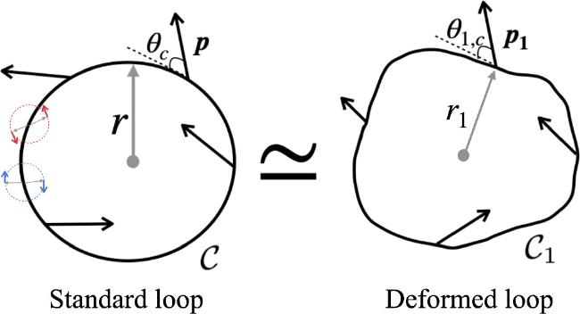
Figure 1. Equivalence between the standard loop ${ \mathcal C }$ and the deformed loop ${{ \mathcal C }}_{1};$ the total number of 2π − rotations of θc in a cyclicality along ${ \mathcal C }$ are composed of n+ positive ‘rotors' (red) and n− negative ‘rotors' (blue). |
KC in Clebsch representation
To prove that ${{\rm{\Gamma }}}_{{ \mathcal C }}$ is quantized, it is most easily done by employing the Clebsch field variables: φ1, φ2 and φ3, with which the velocity and the vorticity take a form of p = φ2∇φ1 + ∇φ3 and ∇ × p = ∇φ2 × ∇φ1, respectively, and the φ3 is determined by the Poisson equation ∇2φ3 = − ∇ · (φ2∇φ1), i.e., the incompressibility condition ∇ · p = 0. The topological structure of the circulation can be revealed by parameterizing the Clebsch fields with the $\hat{{\boldsymbol{n}}}$-field [13], where $\hat{{\boldsymbol{n}}}$ is a 3D vector with a unit length: $\hat{{\boldsymbol{n}}}\cdot \hat{{\boldsymbol{n}}}={n}_{1}^{2}+{n}_{2}^{2}+{n}_{3}^{2}=1$. The φ1 and φ2 fields can be parameterized as φ1 = Zn3 and ${\phi }_{2}=\arg ({n}_{1}+{{in}}_{2})+{\vartheta }_{0}$ where Z is a dimensional constant (independent of time and coordinates) and ϑ0 is a reference phase. The circulation in the configuration space is then transformed into a circulation in the Clebsch space:5 ) is found as6 ) is simply 2π times the winding number times the length of the loop $\gamma ({ \mathcal C })$ plus the contribution of the reference phase. Thus, the existence of a topological number in the KC is proven neatly through the utilization of Clebsch variables. The expression equation (6 ) exhibits a striking resemblance to the helicity in Clebsch representation [11]. The only difference is that the KC is confined to 2D space.
$\begin{eqnarray}{{\rm{\Gamma }}}_{{ \mathcal C }}={\oint }_{\gamma ({ \mathcal C })}{\phi }_{2}{\rm{d}}{\phi }_{1}={\oint }_{{ \mathcal D }({ \mathcal C })}{\rm{d}}{\phi }_{2}\wedge {\rm{d}}{\phi }_{1},\end{eqnarray}$
where $\gamma ({ \mathcal C })$ is the loop in the Clebsch space and ${ \mathcal D }({ \mathcal C })$ is the corresponding area in (φ1, φ2) plane encircled by $\gamma ({ \mathcal C })$. The multi-valuedness of the φ2 field requires introducing a incision along the loop, so as to glue the ${\rm{\Delta }}n^{\prime} $ copies of the Riemann sheets together with ${\rm{\Delta }}n^{\prime} $ the winding number of the φ2 field. The discontinuity of φ2 makes a $2\pi {\rm{\Delta }}n^{\prime} $ contribution to the area integral when crossing the incision line. Then, equation ( $\begin{eqnarray}{{\rm{\Gamma }}}_{{ \mathcal C }}=(2\pi {\rm{\Delta }}n^{\prime} +{\vartheta }_{0}){\oint }_{\gamma ({ \mathcal C })}{\rm{d}}{\phi }_{1},\end{eqnarray}$
where the integral on the RHS is a unit circulation. Equation (Gauge symmetry of the KC
Despite its straightforwardness in extracting the topological number from the circulation, i.e., proving ${{\rm{\Gamma }}}_{{ \mathcal C }}$ to be a topological invariant, the underlying physical process associated with ${\rm{\Delta }}n^{\prime} $ remains hidden in the Clebsch representation. In the following section, we reveal that ${\rm{\Delta }}n^{\prime} $ is precisely the Kelvin's number. To achieve this target, we need to show the equivalence between the gauge invariance and the conservation of the KC.
For convenience, we define two types of loops (figure 1): (1) the standard loop ${ \mathcal C }$, which is a circle with the radius r and the velocity amplitude p being constants, but a varying θc (i.e., dθc/dl ≠ 0) and (2) a deformed loop with varying r1, p1 and θ1,c. It is generally known (e.g., [3]) that the topological invariance of a physical quantity is intimately connected with its invariance under a gauge transformation. To see how gauge invariance enters the KC, we carry out a Galilean transformation on the standard loop ${ \mathcal C }$, i.e., adding a constant shift Δp to p, so that its KC becomes8 ) represents a gauge transformation on the loop integral. It can be rewritten as:
$\begin{eqnarray}{\oint }_{{ \mathcal C }}{\boldsymbol{p}}\cdot {\rm{d}}{\boldsymbol{l}}\to {\oint }_{{ \mathcal C }}{\boldsymbol{p}}\cdot {\rm{d}}{\boldsymbol{l}}+| {\rm{\Delta }}p| {\oint }_{{ \mathcal C }}\cos {\theta }_{{\rm{\Delta }}p}{\rm{d}}l,\end{eqnarray}$
where ${\theta }_{{\rm{\Delta }}p}\in \left[0,2\pi \right]$ is the crossphase between Δp and dl. With dl = rdθΔp, we have $\begin{eqnarray}{\oint }_{{ \mathcal C }}\cos {\theta }_{{\rm{\Delta }}p}{\rm{d}}l=r{\int }_{0}^{2\pi }\cos {\theta }_{{\rm{\Delta }}p}{\rm{d}}{\theta }_{{\rm{\Delta }}p}=0.\end{eqnarray}$
Equation ( $\begin{eqnarray}{\oint }_{{ \mathcal C }}\cos {\theta }_{{\rm{\Delta }}p}{\rm{d}}l=\mathrm{Re}\left(\oint {{\rm{e}}}^{{\rm{i}}{\theta }_{{\rm{\Delta }}p}}{\rm{d}}l\right)=0,\end{eqnarray}$
where ${{\rm{e}}}^{{\rm{i}}{\theta }_{{\rm{\Delta }}p}}$ is an element of the familiar U(1) group. Therefore, the conservation of ${{\rm{\Gamma }}}_{{ \mathcal C }}$ under Galilean transformation is equivalent to a local gauge invariance of the loop. This conclusion can indeed be generalized into the equivalence between a gauge transformation applied to the standard loop and a random stretching on the deformed loop (figure 1).To see it, we start with a standard loop ${ \mathcal C }$ having the same circulation as that of a deformed loop ${{ \mathcal C }}_{1}$, i.e., ${{\rm{\Gamma }}}_{{ \mathcal C }}={{\rm{\Gamma }}}_{{{ \mathcal C }}_{1}}$. A continuous differential deformation of the loop ${{ \mathcal C }}_{1}$ consists of three types of operations: ${\hat{F}}_{\delta {\theta }_{1,c}}$, ${\hat{F}}_{\delta {p}_{1}}$ and ${\hat{F}}_{\delta {l}_{1}}$ representing deformations on θ1,c, p1 and l1, respectively. For the phase deforming operator ${F}_{\delta {\theta }_{1,c}}$, we simply have ${\hat{F}}_{\delta {\theta }_{1,c}}({{\rm{\Gamma }}}_{{{ \mathcal C }}_{1}})\,={\oint }_{{{ \mathcal C }}_{1}}{p}_{1}\cos ({\theta }_{1,c}+\delta {\theta }_{1,c}){\rm{d}}{l}_{1}$. This is equivalent to a phase modulation on the standard loop with $\delta {\theta }_{c}\,=({p}_{1}/p)(\sin {\theta }_{1,c}/\sin {\theta }_{c}){J}_{1}\delta {\theta }_{1,c}$ and the Jacobian J1 = ∣dl1/dl∣, i.e., ${\hat{F}}_{\delta {\theta }_{1,c}}({{\rm{\Gamma }}}_{{{ \mathcal C }}_{1}})={\hat{F}}_{\delta {\theta }_{c}}({{\rm{\Gamma }}}_{C})$. For the amplitude deforming operator ${\hat{F}}_{\delta {p}_{1}}$, we have ${\hat{F}}_{\delta {p}_{1}}({{\rm{\Gamma }}}_{{{ \mathcal C }}_{1}})={\oint }_{{{ \mathcal C }}_{1}}({p}_{1}+\delta {p}_{1})\cos {\theta }_{1,c}{\rm{d}}{l}_{1}$. By introducing a corresponding phase variation $\delta {\theta }_{{p}_{1}}$ and letting $\delta {\theta }_{{p}_{1}}=-(\delta {p}_{1}/{p}_{1})\cos {\theta }_{1,c}$, we have ${\hat{F}}_{\delta {p}_{1}}({{\rm{\Gamma }}}_{{{ \mathcal C }}_{1}})={\hat{F}}_{\delta {\theta }_{{p}_{1}}}({{\rm{\Gamma }}}_{{ \mathcal C }})$, which is again equivalent to a phase modulation on the standard loop. For the loop deforming operator ${\hat{F}}_{\delta {l}_{1}}$, we have ${\hat{F}}_{\delta {l}_{1}}({{\rm{\Gamma }}}_{{{ \mathcal C }}_{1}})={\oint }_{{{ \mathcal C }}_{1}}({p}_{1}+{\dot{p}}_{1}\delta {l}_{1})\cos ({\theta }_{1,c}+{\dot{\theta }}_{1,c}\delta {l}_{1}){\rm{d}}({l}_{1}+\delta {l}_{1})\,={\oint }_{{{ \mathcal C }}_{1}}{p}_{1}\cos {\theta }_{1,c}{\rm{d}}{l}_{1}$ where ${\dot{\theta }}_{1,c}\equiv {\rm{d}}{\theta }_{1,c}/{\rm{d}}{l}_{1}$, ${\dot{p}}_{1}\equiv {\rm{d}}{p}_{1}/{\rm{d}}{l}_{1}$, i.e., ${\hat{F}}_{\delta {l}_{1}}$ is an identity operator and it reflects the invariance of the circulation under reparametrizing the loop. An arbitrary differential deformation of the loop ${{ \mathcal C }}_{1}$ is thus equivalent to a gauge transformation of the standard loop, i.e.,10 ), it becomes clear that the conservation of the KC is equivalent to the gauge symmetry of the standard loop:
$\begin{eqnarray}{\hat{F}}_{\delta {l}_{1}}\circ {\hat{F}}_{\delta {p}_{1}}\circ {\hat{F}}_{\delta {\theta }_{1,c}}({{\rm{\Gamma }}}_{{{ \mathcal C }}_{1}})={\hat{F}}_{\delta \theta }({{\rm{\Gamma }}}_{{ \mathcal C }})=\mathrm{Re}\left(p{\oint }_{{ \mathcal C }}{{\rm{e}}}^{{\rm{i}}({\theta }_{c}+\delta \theta )}{\rm{d}}l\right),\end{eqnarray}$
where the relation between δθ and (δp1, δθ1,c) is given by the proceeded discussions. With the above relation, it becomes evident that a finite distortion on a deformed loop can be decomposed into a series of gauge transformations on the standard loop. This process can be visualized as altering the rotation frequency of p while traveling along ${ \mathcal C }$. Thus, we arrive at a significant conclusion: the deformation of a loop ${{ \mathcal C }}_{1}$ is equivalent to exert a local gauge transformation on the standard loop, thereby mapping any deformed loop to a gauged integral of the standard loop. With relation ( $\begin{eqnarray}{\hat{F}}_{\delta \theta }({{\rm{\Gamma }}}_{{ \mathcal C }})={{\rm{\Gamma }}}_{{ \mathcal C }}.\end{eqnarray}$
Kelvin's number in a laminar flow
Since the deformation of a loop ${{ \mathcal C }}_{1}$ corresponds to a wiggle of the crossphase along a standard loop ${ \mathcal C }$, it is sufficient to calculate the KC associated with the standard loop, which is the gauge integral12 )) can then be decomposed into13 ) becomes6 ), we have ${\rm{\Delta }}n={\rm{\Delta }}n^{\prime} $, ${{\rm{\Gamma }}}_{1}={\oint }_{\gamma ({ \mathcal C })}{\rm{d}}{\phi }_{1}$ and δn0Γ0 = ϑ0Γ1. Thus, using the gauge symmetry of the KC, we obtain the physical meaning of the topological number ${\rm{\Delta }}n^{\prime} $ in Clebsch representation: it is the number of net 2π − rotations in a cyclic along the circulation loop.
$\begin{eqnarray}{{\rm{\Gamma }}}_{{ \mathcal C }}=p\ \mathrm{Re}({\oint }_{{ \mathcal C }}{{\rm{e}}}^{{\rm{i}}{\theta }_{c}}{\rm{d}}l).\end{eqnarray}$
The total 2π-rotations of θc during a cyclic along ${ \mathcal C }$ is composed of n+ anti-clockwise rotations (labeled as positive ‘rotors') and n− clockwise rotations (labeled as negative ‘rotors'), so we have the relations: n = n+ + n− and Δn = n+ − n−. Dividing the loop into n arcs ($L={\sum }_{i}^{n}{L}_{i}$) where each arc Li is associated with a rotor, the integral (equation ( $\begin{eqnarray}{\oint }_{{ \mathcal C }}{{\rm{e}}}^{{\rm{i}}{\theta }_{c}}{\rm{d}}l=\displaystyle \sum _{i=0}^{{n}_{+}}{\int }_{{L}_{i}^{+}}{{\rm{e}}}^{{\rm{i}}{\theta }_{c}}{\rm{d}}l+\displaystyle \sum _{j=0}^{{n}_{-}}{\int }_{{L}_{j}^{-}}{{\rm{e}}}^{{\rm{i}}{\theta }_{c}}{\rm{d}}l+{\delta }_{n0}\oint {{\rm{e}}}^{{\rm{i}}{\theta }_{c}}{\rm{d}}l,\end{eqnarray}$
where δn0 is included to address the case of both n+ = 0 and n− = 0. Due to the gauge symmetry of the circulation, we can always apply a proper gauge transformation to ensure the distributions of all positive (negative) rotors are the same and for n = 0, we simply set θc = 0. Since a positive rotor is transformed into a negative rotor via a reflection operation l → −l, the gauge integral in equation ( $\begin{eqnarray}{\oint }_{{ \mathcal C }}{{\rm{e}}}^{{\rm{i}}{\theta }_{c}}{\rm{d}}l={\rm{\Delta }}n{\int }_{{L}_{1}^{+}}{{\rm{e}}}^{{\rm{i}}{\theta }_{c}}{\rm{d}}l+{\delta }_{n0}{L}_{0},\end{eqnarray}$
and the total circulation along ${ \mathcal C }$ is then $\begin{eqnarray}{{\rm{\Gamma }}}_{{ \mathcal C }}=2\pi {\rm{\Delta }}n{{\rm{\Gamma }}}_{1}+{\delta }_{n0}{{\rm{\Gamma }}}_{0},\end{eqnarray}$
where Δn = n+ − n−, ${{\rm{\Gamma }}}_{1}=p{\int }_{{L}_{1}^{+}}{{\rm{e}}}^{{\rm{i}}{\theta }_{c}}{\rm{d}}l/(2\pi )$ is the circulation carried by a positive rotor and Γ0 ≡ pL. Comparing with equation (Kelvin's number in a turbulent flow
The stochastic nature of a turbulence system renders both p and θc as stochastic variables, with l serving as their internal parameter, i.e., p = p(l) and θc = θc(l). By reparametrizing dl into ${\rm{d}}l={\rm{d}}{\theta }_{c}/{\dot{\theta }}_{c}$ with ${\dot{\theta }}_{c}\equiv {\rm{d}}{\theta }_{c}/{dl}$ the rotation frequency of θc along the loop, we have p(l) → p(θc). With the gauge invariance, each rotor has the same distribution. The gauge integral for a stochastic crossphase is recast as16 ). For the stochastic process, a standard way to calculate the integral in equation (16 ) is using the invariant measure, i.e., the probability distribution function ρ+ (ρ−) of the positive (negative) rotor. ρ± satisfies the conservation equation19 ) is the same as the definition of complex order parameter used in the phase synchronization model of oscillators in many-body systems [14], and it is defined as:17 ) is symmetrical under the l − reversal transformation, a positive rotor can be mapped into a negative rotor through a reversal: l → −l, which is similar to the time reversal operation. Under this transformation, we obtain ρ−(l) = ρ+( − l). When θc reaches a statistical equilibrium state, we have ρ+(l) = ρ+( − l) ≡ ρ(l) and the following relations:19 ) and (20 ), the KC is obtained as:22 ) has a similar form to equation (15 ). For a turbulence system, the unit circulation Γ1 is a continuous stochastic quantity and its distribution relies on the statistical mechanics of the circulations [11]. In the extraction of the topological number in ΓC for turbulent fluids, we solely used the gauge symmetry of the KC without invoking any specific properties pertaining to the turbulence field.
$\begin{eqnarray}\begin{array}{l}{\oint }_{{ \mathcal C }}{{\rm{e}}}^{{\rm{i}}{\theta }_{c}}{\rm{d}}l={n}_{+}{\int }_{{L}_{1}^{+}}\displaystyle \frac{{{\rm{e}}}^{{\rm{i}}{\theta }_{c}}}{{\dot{\theta }}_{c}}{\rm{d}}{\theta }_{c}\\ \,+{n}_{-}{\int }_{{L}_{1}^{-}}\displaystyle \frac{{{\rm{e}}}^{{\rm{i}}{\theta }_{c}}}{{\dot{\theta }}_{c}}{\rm{d}}{\theta }_{c}+{\delta }_{n0}\oint {{\rm{e}}}^{{\rm{i}}{\theta }_{c}}{\rm{d}}l,\end{array}\end{eqnarray}$
where ${\dot{\theta }}_{c}$ is a weighting function: θc has a prolonged dwelling time in the lower rotation frequency regime, thereby amplifying the contribution of ${e}^{{\rm{i}}{\theta }_{c}}$ to the integral, which is reflected by a larger $1/| {\dot{\theta }}_{c}| $ and vice versa. For a positive rotor, we have ${\dot{\theta }}_{c}\gt 0$ and for a negative rotor, ${\dot{\theta }}_{c}\lt 0$. In general ${\dot{\theta }}_{c}$ varies with θc, i.e., ${\rm{d}}{\dot{\theta }}_{c}/{\rm{d}}{\theta }_{c}\ne 0$ and one cannot move it out of the integral in equation ( $\begin{eqnarray}{\partial }_{l}{\rho }_{\pm }+{\partial }_{{\theta }_{c}}({\dot{\theta }}_{c}{\rho }_{\pm })=0.\end{eqnarray}$
For ‘stationary' distribution ∂lρ± = 0, one has ${\dot{\theta }}_{c}{\rho }_{\pm }=$ constant and the distribution function is obtained as: $\begin{eqnarray}{\rho }_{\pm }=\displaystyle \frac{{H}_{\pm }}{{\dot{\theta }}_{c}},\end{eqnarray}$
with H± the normalization constants. The positiveness of ρ± requires $\mathrm{sign}({H}_{\pm })=\mathrm{sign}({\dot{\theta }}_{c})$, i.e., H+ > 0 and H− < 0. The phase integral associated with each rotor is: $\begin{eqnarray}{\int }_{{L}_{1}^{\pm }}{{\rm{e}}}^{{\rm{i}}{\theta }_{c}}{\rm{d}}l={H}_{\pm }{\int }_{0}^{2\pi }{{\rm{e}}}^{{\rm{i}}{\theta }_{c}}{\rho }_{\pm }{\rm{d}}{\theta }_{c}.\end{eqnarray}$
It is enlightening to observe that the statistical average over ${e}^{{\rm{i}}{\theta }_{c}}$ on the RHS of equation ( $\begin{eqnarray}{R}_{\pm }\triangleq {\int }_{0}^{2\pi }{{\rm{e}}}^{{\rm{i}}{\theta }_{c}}{\rho }_{\pm }{\rm{d}}{\theta }_{c}.\end{eqnarray}$
Using the amplitude-phase decomposition, one has ${R}_{\pm }=| {R}_{\pm }| {{\rm{e}}}^{i{{\rm{\Theta }}}_{\pm }}$ with 0 ≤ ∣R±∣ ≤ 1 the real order parameter and Θ± the phase order parameter. For ∣R±∣ = 0, it corresponds to a uniform distribution and ∣R±∣ = 1 corresponds to a constant crossphase along the standard loop. As equation ( $\begin{eqnarray}{H}_{+}=-{H}_{-}\equiv H\,\mathrm{and}\,{R}_{+}={R}_{-}\equiv R.\end{eqnarray}$
Substituting the above relations into equations ( $\begin{eqnarray}{{\rm{\Gamma }}}_{{C}}=2\pi {\rm{\Delta }}n{{\rm{\Gamma }}}_{1}+{\delta }_{n0}{{\rm{\Gamma }}}_{0},\end{eqnarray}$
with the unit excitation $\begin{eqnarray*}{{\rm{\Gamma }}}_{1}\equiv \displaystyle \frac{1}{2\pi }{pH}\mathrm{Re}(R).\end{eqnarray*}$
Equation (On the distribution of Δn
By taking the 2π − rotors as the basic blocks of a circulation, a natural subsequent question is how the rotors distribute along the loop? We address this issue by fixing the total number (n) of the rotors. Treating each loop as a micro-canonical system, the degeneracy Ω(Δn) (number of state) of the circulation is then the number of ways of permuting the n rotors and it is
$\begin{eqnarray}{\rm{\Omega }}({\rm{\Delta }}n)=\displaystyle \frac{n!}{{n}_{+}!{n}_{-}!},\end{eqnarray}$
where n+ = (n + Δn)/2 and n− = (n − Δn)/2. It is interesting to note that Ω is a decreasing function of Δn, with its maximum value being at Δn = 0. From the viewpoint of statistic physics, the inverse of the effective temperature is given as $\begin{eqnarray}\beta =\displaystyle \frac{1}{{k}_{{\rm{B}}}T}=\displaystyle \frac{\partial }{\partial {{\rm{\Gamma }}}_{{ \mathcal C }}}{\rm{\Omega }}=\displaystyle \frac{1}{2\pi {{\rm{\Gamma }}}_{1}}\displaystyle \frac{\partial }{\partial {\rm{\Delta }}n}{\rm{\Omega }}.\end{eqnarray}$
So that the relative distribution Δn/n is obtained as $\begin{eqnarray}\displaystyle \frac{{\rm{\Delta }}n}{n}=\displaystyle \frac{{{\rm{e}}}^{-4\pi \beta {{\rm{\Gamma }}}_{1}}-1}{{{\rm{e}}}^{-4\pi \beta {{\rm{\Gamma }}}_{1}}+1}\end{eqnarray}$
Δn/n is a monotonic function of the unit circulation. ∣Δn/n∣ becomes larger with the increase of ∣Γ1∣.Discussions
In this work, we uncover a hidden symmetry in the fluid dynamics–the topological invariant/number in Kelvin's circulation. It is interesting to observe that the circulation of a loop is a combination of a discrete variable (i.e., the integer Δn) and a continuous variable (i.e., Γ1) in the inviscid classical fluids. One can expect that when including the viscosity effect, the topological number may still survive for a continuous dissipation process. This is because any variation of Δn would induce a ‘jump' of the total circulation, which is in contradiction with the continuous dissipation assumption.