


1. Introduction
The development of mathematics has often benefited from problems found in physics, and every major revolution in physics has been associated with the introduction of new mathematical knowledge. For example, theoretical mechanics and calculus theory [1]; electromagnetic theory and fiber bundles theory [2]; gravitational waves and Riemannian geometry [3]; quantum theory and quantum mechanics (the development of quantum mechanics builds on linear algebra in mathematics) [4]. We often use mathematical tools to describe some physical problems, for example, using nonlinear partial differential equations (PDEs) and nonlinear evolution equations (NLEEs) to describe phenomena in optics, fluid mechanics, plasma physics, biology, engineering, applied physics [5], etc. Obviously, finding solutions of nonlinear partial differential equations is an extremely complex and important task.
With the rapid development of nonlinear science in the past few decades, many effective and reliable methods have been developed to solve exact solutions of nonlinear PDEs such as inverse scattering transform [6], Hirota's bilinear method [7], Darboux transformation [8], Painlevé analysis [9, 10], Lie symmetry analysis [11], the homogeneous balance method [12], the Jacobian elliptic function expansion method [13], etc. But these traditional methods face great challenges in tackling many nonlinear problems because of the complexity and variability of nonlinear phenomena.
Symmetry analysis [14, 15] plays an important role in both simplifying nonlinear PDEs and obtaining their exact solutions. Thanks to Lie's first theorem, one can find finite transformation corresponding to a Lie point symmetry group. Using the classical Lie group method, we could get both Lie symmetry group and symmetry reduction solutions for many integrable systems in a standard way. However, nonlocal symmetry [16, 17], which plays an important role in the study of nonlinear systems, cannot be obtained in a unified way. Nonetheless, we can obtain nonlocal symmetries for some nonlinear systems through different ways such as inverse recursion operators [18], Lax pairs [19], Bäcklund transformation [20], conformal invariance [21], potential symmetries [22], etc.
Recently, Lou found that for a Painlevé integrable system the residue of a truncated Painlevé expansion with respect to a singular manifold is actually a nonlocal symmetry of the system , which is called residual symmetry. For many nonlinear systems, it is interesting that residual symmetry could be localized into a Lie point symmetry in a prolonged system by introducing appropriate new dependent variables. In real nature, interaction solutions between solitons and nonlinear waves often occur under various physical backgrounds and many of which are observed experimentally [23]. It is found that symmetry reduction solutions related to residual symmetry include this type of interaction solution [24]. Moreover, a localization procedure for nonlocal symmetry can also used to get Nth Bäcklund transformations for many integrable equations [25, 26]. In another aspect, Lou generalized the Riccati expansion method to the consistent Riccati expansion (CRE) method and defined a new integrable property called CRE integrable [27]. It turns out that the CRE method is effective for obtaining interaction solutions between solitons and periodic waves [28, 29].
The coupled nonlinear evolution equation system, the Drinfeld–Sokolov–Satsuma–Hirota (DSSH) system, independently, was proposed by Drinfeld and Sololov [30], and by Satsuma and Hirota [31], which takes the form
$\begin{eqnarray}{u}_{t}=\displaystyle \frac{1}{2}{u}_{{xxx}}-3{{uu}}_{x}+3{v}_{x},\end{eqnarray}$
and $\begin{eqnarray}{v}_{t}=-{v}_{{xxx}}+3{{uv}}_{x},\end{eqnarray}$
where u, v are two long wave functions with different dispersion relation [32]. The DSSH system is a special case of the four-reduced Kadomstev–Petviashvili hierarchy [31] and it is a basic model for representing many physical phenomena in shallow water and coastal regions [33]. In recent years, the DSSH system has been studied in many different aspects. In [32], the authors obtained its trigonometric function traveling wave solutions, hyperbolic function traveling wave solutions and rational function traveling wave solutions by using the modified polynomial expansion method. In [33], the authors found analytical solutions by using the enhanced modifed extended tanh method (eMETEM) and the unified Riccati equation expansion (UREEM). In [34], the authors discussed nonlocal symmetry of this system and obtained its similarity reductions by using the classical Lie group approach. In [35], the authors constructed an explicit Bäcklund transformation of this system by using the Weiss method of truncated singular expansions and found some special solutions under this transformation. In [36], the authors obtained soliton solutions, multiple soliton solutions, multiple singular soliton solutions and plane periodic solutions by using the Cole–Hopf transformation method, the tanh–coth method and the Exp-function method, respectively. In [37], the authors constructed a Darboux transformation of this system to obtain several types of solutions including soliton solutions, periodic solutions, rational solutions. In [38], the authors considered the iterations of the Darboux transformation obtained in [37] and obtained new solutions of the DSSH system given in terms of determinants.The paper is organized as follows. In section 2 , residual symmetries of the DSSH system (1 ) and (2 ) are obtained and localized in a prolonged system which leads to a new Bäcklund transformation of the system by using Lie's first theorem. In section 3 , by applying the classical Lie group approach to the prolonged DSSH system, the general form of Lie point symmetry group and corresponding symmetry reduction solutions are obtained. In section 4 , some new Bäcklund transformations of the DSSH system are generated by using the CRE and consistent tanh expansion (CTE) method, from which interaction solutions between solitons and periodic waves are illustrated. The last section is devoted to a short summary.
2. Residual symmetry and its localization
By balancing the dispersion term and highest order nonlinear term, the truncated Painlevé expansion of the DSSH system is taken as3 ) and (4 ) into (1 ) and (2 ) and vanishing all different powers of $\tfrac{1}{\phi }$, the results are
$\begin{eqnarray}u=\displaystyle \frac{{u}_{0}}{{\phi }^{2}}+\displaystyle \frac{{u}_{1}}{\phi }+{u}_{2},\end{eqnarray}$
$\begin{eqnarray}v=\displaystyle \frac{{v}_{0}}{\phi }+{v}_{1},\end{eqnarray}$
where φ is a singular manifold and u0, u1, u2, v0, v1 are functions of x, t, which are determined by substituting equations ( $\begin{eqnarray}{u}_{0}=2{\phi }_{x}^{2},{u}_{1}=-2{\phi }_{{xx}},\end{eqnarray}$
$\begin{eqnarray}{u}_{2}=-\displaystyle \frac{2{\phi }_{t}{\phi }_{x}-4{\phi }_{x}{\phi }_{{xxx}}+3{\phi }_{{xx}}^{2}}{6{\phi }_{x}^{2}},\end{eqnarray}$
and $\begin{eqnarray}\begin{array}{rcl}{v}_{0} & = & -\displaystyle \frac{1}{3{\phi }_{x}^{2}}(2{\phi }_{{xt}}{\phi }_{x}^{2}-{\phi }_{{xxxx}}{\phi }_{x}^{2}\\ & & -2{\phi }_{t}{\phi }_{x}{\phi }_{{xx}}+4{\phi }_{{xx}}{\phi }_{{xxx}}{\phi }_{x}-3{\phi }_{{xx}}^{3}),\end{array}\end{eqnarray}$
$\begin{eqnarray}\begin{array}{rcl}{v}_{1} & = & -\displaystyle \frac{1}{144{\phi }_{x}^{4}}\left\{24({\phi }_{5x}-2{\phi }_{{xxt}}){\phi }_{x}^{3}\right.\\ & & +[64{\phi }_{{xxx}}{\phi }_{t}-100{\phi }_{{xxx}}^{2}\\ & & +48({\phi }_{{xt}}-2{\phi }_{4x}){\phi }_{{xx}}-16{\phi }_{t}^{2}]{\phi }_{x}^{2}\\ & & \left.+(324{\phi }_{{xx}}^{2}{\phi }_{{xxx}}-72{\phi }_{{xx}}^{2}{\phi }_{t}){\phi }_{x}-153{\phi }_{{xx}}^{4}\right\}.\end{array}\end{eqnarray}$
Then the DSSH system is reduced to its Schwarzian form $\begin{eqnarray}{C}_{t}(3K+C){C}_{x}+2{K}_{t}+2(K-C){K}_{x}-{C}_{{xxx}}=0,\end{eqnarray}$
where $C=\tfrac{{\phi }_{{xxx}}}{{\phi }_{x}}-\tfrac{3}{2}\tfrac{{\phi }_{{xx}}^{2}}{{\phi }_{x}^{2}}$, $K=\tfrac{{\phi }_{t}}{{\phi }_{x}}$ are Schwarzian variables.After substituting equations (5 ) and (6 ) into (3 ) and equations (7 ) and (8 ) into (4 ), respectively, we get a new Bäcklund transformation for the DSSH system.
Theorem 1. If φ is a solution of the Schwartzian equation (9 ), then5 ) and (7 ) satisfy linearized equations of equations (1 ) and (2 ) which can be easily verified, so it is a symmetry of the DSSH system which is called residual symmetry.
$\begin{eqnarray}u=-\displaystyle \frac{{\phi }_{t}}{3{\phi }_{x}}+\displaystyle \frac{2{\phi }_{x}^{2}}{{\phi }^{2}}-\displaystyle \frac{2{\phi }_{{xx}}}{\phi }+\displaystyle \frac{2{\phi }_{{xxx}}}{3{\phi }_{x}}-\displaystyle \frac{{\phi }_{{xx}}^{2}}{2{\phi }_{x}^{2}},\end{eqnarray}$
$\begin{eqnarray}\begin{array}{rcl}v & = & -\displaystyle \frac{1}{3{\phi }_{x}^{2}\phi }(2{\phi }_{{xt}}{\phi }_{x}^{2}-{\phi }_{{xxxx}}{\phi }_{x}^{2}-2{\phi }_{t}{\phi }_{x}{\phi }_{{xx}}\\ & & +4{\phi }_{{xx}}{\phi }_{{xxx}}{\phi }_{x}-3{\phi }_{{xx}}^{3})\\ & & -\displaystyle \frac{1}{144{\phi }_{x}^{4}}\left\{24({\phi }_{5x}-2{\phi }_{{xxt}}){\phi }_{x}^{3}\right.\\ & & +[64{\phi }_{{xxx}}{\phi }_{t}-100{\phi }_{{xxx}}^{2}\\ & & +48({\phi }_{{xt}}-2{\phi }_{4x}){\phi }_{{xx}}-16{\phi }_{t}^{2}]{\phi }_{x}^{2}\\ & & \left.+(324{\phi }_{{xx}}^{2}{\phi }_{{xxx}}-72{\phi }_{{xx}}^{2}{\phi }_{t}){\phi }_{x}-153{\phi }_{{xx}}^{4}\right\},\end{array}\end{eqnarray}$
is a solution of the DSSH system. It is clear that any equations of Schwarzian form are invariant under Möbious transformation $\begin{eqnarray}\phi \longrightarrow \displaystyle \frac{a\phi +b}{c\phi +d},{ac}\ne {bd},\end{eqnarray}$
which means that these types of equations have symmetries σφ = d1, σφ = d2φ and $\begin{eqnarray}{\sigma }_{\phi }={d}_{3}{\phi }^{2},\end{eqnarray}$
where d1, d2 and d3 are arbitrary constants. It is interesting that u1 and v0 in equations (It is obvious that a residual symmetry is nonlocal which cannot be used directly by Lie's first fundamental theorem to generate its finite transformation. To concur this difficulty we localize the residual symmetry in a new prolonged DSSH system by introducing five new dependent variables
$\begin{eqnarray}g\equiv {\phi }_{x},h\equiv {g}_{x},m\equiv {h}_{x},n\equiv {m}_{x},p\equiv {u}_{x}.\end{eqnarray}$
By fixing the symmetry of φ as σφ = φ2 and using the equations in the prolonged DSSH system, it can be verified that the Lie point symmetry1 ), (2 ), (9 ) and (14 ), which means the residual symmetry is successfully localized in the prolonged DSSH system. Meanwhile, the symmetry of (15a ) can also be expressed in vector form as
$\begin{eqnarray}{\sigma }_{u}=2h,\end{eqnarray}$
$\begin{eqnarray}{\sigma }_{v}=-\displaystyle \frac{2{g}^{3}p-{g}^{2}n+2{ghm}-{h}^{3}}{{g}^{2}},\end{eqnarray}$
$\begin{eqnarray}{\sigma }_{\phi }={\phi }^{2},\end{eqnarray}$
$\begin{eqnarray}{\sigma }_{g}=2g\phi ,\end{eqnarray}$
$\begin{eqnarray}{\sigma }_{h}=2{g}^{2}+2h\phi ,\end{eqnarray}$
$\begin{eqnarray}{\sigma }_{m}=6{gh}+2m\phi ,\end{eqnarray}$
$\begin{eqnarray}{\sigma }_{n}=8{gm}+6{h}^{2}+2n\phi ,\end{eqnarray}$
$\begin{eqnarray}{\sigma }_{p}=2m,\end{eqnarray}$
satisfies the linearized system of ( $\begin{eqnarray}\begin{array}{rcl}V & = & 2h{\partial }_{u}-\displaystyle \frac{2{g}^{3}p-{g}^{2}n+2{ghm}-{h}^{3}}{{g}^{2}}\\ & & \times {\partial }_{v}+{\phi }^{2}{\partial }_{\phi }+2g\phi {\partial }_{g}+(2{g}^{2}+2h\phi ){\partial }_{h}\\ & & +(6{gh}+2m\phi ){\partial }_{m}+(8{gm}+6{h}^{2}+2n\phi ){\partial }_{n}+2m{\partial }_{p}.\end{array}\end{eqnarray}$
According to Lie's first fundamental theorem, after solving the corresponding initial value problem of (16 ), which is
$\begin{eqnarray}\displaystyle \frac{{\rm{d}}\hat{u}(\epsilon )}{{\rm{d}}\epsilon }=2\hat{h}(\epsilon ),\quad \hat{u}(0)=u,\end{eqnarray}$
$\begin{eqnarray}\begin{array}{rcl}\displaystyle \frac{{\rm{d}}\hat{v}(\epsilon )}{{\rm{d}}\epsilon } & = & -\displaystyle \frac{2\hat{g}{\left(\epsilon \right)}^{3}\hat{p}(\epsilon )-\hat{g}{\left(\epsilon \right)}^{2}\hat{n}(\epsilon )+2\hat{g}(\epsilon )\hat{h}(\epsilon )\hat{m}(\epsilon )-\hat{h}{\left(\epsilon \right)}^{3}}{\hat{g}{\left(\epsilon \right)}^{2}},\\ \hat{v}(0) & = & v,\end{array}\end{eqnarray}$
$\begin{eqnarray}\displaystyle \frac{{\rm{d}}\hat{g}(\epsilon )}{{\rm{d}}\epsilon }=2\hat{\phi }(\epsilon )\hat{g}(\epsilon ),\quad \hat{g}(0)=g,\end{eqnarray}$
$\begin{eqnarray}\displaystyle \frac{{\rm{d}}\hat{\phi }(\epsilon )}{{\rm{d}}\epsilon }=\hat{\phi }{\left(\epsilon \right)}^{2},\quad \hat{\phi }(0)=\phi ,\end{eqnarray}$
$\begin{eqnarray}\displaystyle \frac{{\rm{d}}\hat{h}(\epsilon )}{{\rm{d}}\epsilon }=2\hat{g}{\left(\epsilon \right)}^{2}+2\hat{h}(\epsilon )\hat{\phi }(\epsilon ),\quad \hat{h}(0)=h,\end{eqnarray}$
$\begin{eqnarray}\displaystyle \frac{{\rm{d}}\hat{m}(\epsilon )}{{\rm{d}}\epsilon }=6\hat{g}(\epsilon )\hat{h}(\epsilon )+2\hat{m}(\epsilon )\hat{\phi }(\epsilon ),\quad \hat{m}(0)=m,\end{eqnarray}$
$\begin{eqnarray}\displaystyle \frac{{\rm{d}}\hat{n}(\epsilon )}{{\rm{d}}\epsilon }=8\hat{g}(\epsilon )m+6\hat{h}{\left(\epsilon \right)}^{2}+2\hat{n}(\epsilon )\hat{\phi }(\epsilon ),\quad \hat{n}(0)=n,\end{eqnarray}$
$\begin{eqnarray}\displaystyle \frac{{\rm{d}}\hat{p}(\epsilon )}{{\rm{d}}\epsilon }=2\hat{m}(\epsilon ),\quad \hat{p}(0)=p,\end{eqnarray}$
we get the following theorem.Theorem 2. If {u, v, φ, g, h, m, n, p} is a solution of the prolonged system (1 ), (2 ), (9 ), (14 ), then so is $\{\hat{u},\hat{v},\hat{\phi },\hat{g},\hat{h},\hat{m},\hat{n},\hat{p}\}$ with
$\begin{eqnarray}\hat{u}=u+\displaystyle \frac{2{\epsilon }^{2}{g}^{2}-2{\epsilon }^{2}h\phi +2\epsilon h}{{\left(\epsilon \phi -1\right)}^{2}},\end{eqnarray}$
$\begin{eqnarray}\hat{v}=u+\displaystyle \frac{2{\epsilon }^{2}{g}^{2}-2{\epsilon }^{2}h\phi +2\epsilon h}{{\left(\epsilon \phi -1\right)}^{2}},\end{eqnarray}$
$\begin{eqnarray}\hat{\phi }=-\displaystyle \frac{\phi }{\epsilon \phi -1},\end{eqnarray}$
$\begin{eqnarray}\hat{g}=\displaystyle \frac{g}{{\left(\epsilon \phi -1\right)}^{2}},\end{eqnarray}$
$\begin{eqnarray}\hat{h}=-\displaystyle \frac{2\epsilon {g}^{2}-\epsilon h\phi +h}{{\left(\epsilon \phi -1\right)}^{3}},\end{eqnarray}$
$\begin{eqnarray}\hat{m}=\displaystyle \frac{{\epsilon }^{2}m{\phi }^{2}+(-6{\epsilon }^{2}{gh}-2\epsilon m)\phi +6{\epsilon }^{2}{g}^{3}+6\epsilon {hg}+m}{{\left(\epsilon \phi -1\right)}^{4}},\end{eqnarray}$
$\begin{eqnarray}\begin{array}{rcl}\hat{n} & = & -\displaystyle \frac{1}{{\left(\epsilon \phi -1\right)}^{5}}[-{\epsilon }^{3}n{\phi }^{3}+(8{\epsilon }^{3}{gm}+6{\epsilon }^{3}{h}^{2}+3{\epsilon }^{2}n)\\ & & \times {\phi }^{2}+(-36{\epsilon }^{3}{g}^{2}h-16{\epsilon }^{2}{gm}-12{\epsilon }^{2}{h}^{2}-3\epsilon n)\\ & & \times \phi +24{\epsilon }^{3}{g}^{4}+36{\epsilon }^{2}{{hg}}^{2}+8\epsilon {mg}+6\epsilon {h}^{2}+n],\end{array}\end{eqnarray}$
$\begin{eqnarray}\hat{p}=p-\displaystyle \frac{2\epsilon (2{\epsilon }^{2}{g}^{3}-3{\epsilon }^{2}{gh}\phi +{\epsilon }^{2}m{\phi }^{2}+3\epsilon {gh}-2\epsilon m\phi +m)}{{\left(\epsilon \phi -1\right)}^{3}},\end{eqnarray}$
where ε is an arbitrary group parameter.3. Residual symmetry reduction solutions
In this section, we first investigate the general form of Lie point symmetry of the prolonged DSSH system (1 ), (2 ), (9 ), and (14 ), which can be written in a vector form as
$\begin{eqnarray}\begin{array}{rcl}V & = & X\displaystyle \frac{\partial }{\partial x}+T\displaystyle \frac{\partial }{\partial t}+U\displaystyle \frac{\partial }{\partial u}+V\displaystyle \frac{\partial }{\partial v}+{\rm{\Phi }}\displaystyle \frac{\partial }{\partial \phi }\\ & & +G\displaystyle \frac{\partial }{\partial g}+H\displaystyle \frac{\partial }{\partial h}+M\displaystyle \frac{\partial }{\partial m}+N\displaystyle \frac{\partial }{\partial n}+P\displaystyle \frac{\partial }{\partial p},\end{array}\end{eqnarray}$
or in function form as $\begin{eqnarray}{\sigma }_{u}={{Xu}}_{x}+{{Tu}}_{t}-U,\end{eqnarray}$
$\begin{eqnarray}{\sigma }_{v}={{Xv}}_{x}+{{Tv}}_{t}-V,\end{eqnarray}$
$\begin{eqnarray}{\sigma }_{\phi }=X{\phi }_{x}+T{\phi }_{t}-{\rm{\Phi }},\end{eqnarray}$
$\begin{eqnarray}{\sigma }_{g}={{Xg}}_{x}+{{Tg}}_{t}-G,\end{eqnarray}$
$\begin{eqnarray}{\sigma }_{h}={{Xh}}_{x}+{{Th}}_{t}-H,\end{eqnarray}$
$\begin{eqnarray}{\sigma }_{m}={{Xm}}_{x}+{{Tm}}_{t}-M,\end{eqnarray}$
$\begin{eqnarray}{\sigma }_{n}={{Xn}}_{x}+{{Tn}}_{t}-N,\end{eqnarray}$
$\begin{eqnarray}{\sigma }_{p}={{Xp}}_{x}+{{Tp}}_{t}-P,\end{eqnarray}$
which means that the prolonged DSSH system is invariant under the transformation $\begin{eqnarray}\begin{array}{l}\{x,t,u,v,\phi ,g,h,m,n,p\}\to \{x+\epsilon X,t+\epsilon T,\\ u+\epsilon U,v+\epsilon V,\phi +\epsilon {\rm{\Phi }},g+\epsilon G,h+\epsilon H,\\ m+\epsilon M,n+\epsilon N,p+\epsilon P\}.\end{array}\end{eqnarray}$
By substituting (27a ) into the linearized equations of the prolonged DSSH system (1 ), (2 ), (9 ), (14 ) and vanishing all coefficients of different derivatives of u, v, g, h, m, n, p and φ with respect to x, t, we get many linear equations for the infinitesimals X, T, U, V, G, H, Φ, M, N, P which are over-determined, calculated by Maple, we have
$\begin{eqnarray}\begin{array}{rcl}X & = & \displaystyle \frac{{c}_{1}x}{3}+{c}_{4},T={c}_{1}t+{c}_{2},U=-\displaystyle \frac{2}{3}{c}_{1}u-2{c}_{3}h,\\ V & = & 2{c}_{3}{gp}-\displaystyle \frac{4{c}_{1}}{3}v-\displaystyle \frac{{c}_{3}{h}^{3}}{{g}^{2}}+\displaystyle \frac{2{c}_{3}{hm}}{g}-{c}_{3}n,\\ G & = & -\displaystyle \frac{g}{3}(6{c}_{3}\phi +{c}_{1}-3{c}_{5}),H=-2{c}_{3}{g}^{2}-2{c}_{3}\phi h\\ & & +{c}_{5}h-\displaystyle \frac{2}{3}{c}_{1}h,{\rm{\Phi }}=-{c}_{3}{\phi }^{2}+{c}_{5}\phi +{c}_{6},\\ M & = & -6{c}_{3}{gh}-2{c}_{3}m\phi -{c}_{1}m+{c}_{5}m,\\ N & = & -8{c}_{3}{gm}-2{c}_{3}n\phi +{c}_{5}n-\displaystyle \frac{4}{3}{c}_{1}n-6{c}_{3}{h}^{2},\\ P & = & -{c}_{1}p-2{c}_{3}m,\end{array}\end{eqnarray}$
where ci(i = 1, 2, ⋯ ,6) are arbitrary constants.The function form of equation (27a ) can now be written explicitly as30 ) we could get group invariant solutions of the prolonged system (1 ), (2 ), (9 ) and (14 ). We discuss it in the following two cases:
$\begin{eqnarray}\begin{array}{rcl}{\sigma }_{u} & = & (\displaystyle \frac{{c}_{1}x}{3}+{c}_{4}){u}_{x}+({c}_{1}t+{c}_{2}){u}_{t}+\displaystyle \frac{2}{3}{c}_{1}u+2{c}_{3}h,\\ {\sigma }_{v} & = & (\displaystyle \frac{{c}_{1}x}{3}+{c}_{4}){v}_{x}+({c}_{1}t+{c}_{2}){v}_{t}\\ & & -2{c}_{3}{gp}+\displaystyle \frac{4{c}_{1}}{3}v+\displaystyle \frac{{c}_{3}{h}^{3}}{{g}^{2}}-\displaystyle \frac{2{c}_{3}{hm}}{g}+{c}_{3}n,\\ {\sigma }_{\phi } & = & (\displaystyle \frac{{c}_{1}x}{3}+{c}_{4}){\phi }_{x}+({c}_{1}t+{c}_{2}){\phi }_{t}+{c}_{3}{\phi }^{2}-{c}_{5}\phi -{c}_{6},\\ {\sigma }_{g} & = & (\displaystyle \frac{{c}_{1}x}{3}+{c}_{4}){g}_{x}+({c}_{1}t+{c}_{2}){g}_{t}+\displaystyle \frac{g}{3}(6{c}_{3}\phi +{c}_{1}-3{c}_{5}),\\ {\sigma }_{h} & = & (\displaystyle \frac{{c}_{1}x}{3}+{c}_{4}){h}_{x}+({c}_{1}t+{c}_{2}){h}_{t}\\ & & +2{c}_{3}{g}^{2}+2{c}_{3}\phi h-{c}_{5}h+\displaystyle \frac{2}{3}{c}_{1}h,\\ {\sigma }_{m} & = & (\displaystyle \frac{{c}_{1}x}{3}+{c}_{4}){m}_{x}+({c}_{1}t+{c}_{2}){m}_{t}\\ & & +6{c}_{3}{gh}+2{c}_{3}m\phi +{c}_{1}m-{c}_{5}m,\\ {\sigma }_{n} & = & (\displaystyle \frac{{c}_{1}x}{3}+{c}_{4}){n}_{x}+({c}_{1}t+{c}_{2}){n}_{t}\\ & & +8{c}_{3}{gm}+2{c}_{3}n\phi -{c}_{5}n+\displaystyle \frac{4}{3}{c}_{1}n+6{c}_{3}{h}^{2},\\ {\sigma }_{p} & = & (\displaystyle \frac{{c}_{1}x}{3}+{c}_{4}){p}_{x}+({c}_{1}t+{c}_{2}){p}_{t}+{c}_{1}p+2{c}_{3}m.\end{array}\end{eqnarray}$
By using symmetry constraints σu = σv = σφ = σg =σh = σm = σn = σp = 0 in equation (Case 1. ci ≠ 0 (i = 1, 2, ⋯ ,6). In the case, we get
$\begin{eqnarray}\begin{array}{rcl}\phi & = & \displaystyle \frac{{\delta }_{1}\tanh (\tfrac{{F}_{1}}{2})+{c}_{5}}{2{c}_{3}},{\delta }_{1}=\sqrt{4{c}_{3}{c}_{6}+{c}_{5}^{2}},\\ {F}_{1} & = & \displaystyle \frac{{\delta }_{1}({c}_{1}{\rm{\Phi }}+\mathrm{ln}({c}_{1}t+{c}_{2}))}{{c}_{1}},\end{array}\end{eqnarray}$
$\begin{eqnarray}g=-\displaystyle \frac{2G}{{\left({c}_{1}t+{c}_{2}\right)}^{\tfrac{1}{3}}\left[\cosh ({F}_{1})+1\right]},\end{eqnarray}$
$\begin{eqnarray}h=\displaystyle \frac{2[8{G}^{2}{c}_{3}-H{\delta }_{1}\exp ({F}_{1})-H{\delta }_{1}]}{{\delta }_{1}{\left({c}_{1}t+{c}_{2}\right)}^{\tfrac{2}{3}}(\exp ({F}_{1})+1)(\cosh ({F}_{1})+1)},\end{eqnarray}$
$\begin{eqnarray}m=-\displaystyle \frac{M{\delta }_{1}^{2}\exp (2{F}_{1})-2{\delta }_{1}(12{c}_{3}{GH}-M{\delta }_{1})\exp ({F}_{1})+96{c}_{3}^{2}{G}^{3}-24{c}_{3}H{\delta }_{1}G+M{\delta }_{1}^{2}}{{\delta }_{1}^{2}({c}_{1}t+{c}_{2}){\left(\exp ({F}_{1})+1\right)}^{2}(\cosh ({F}_{1})+1)},\end{eqnarray}$
$\begin{eqnarray}\begin{array}{rcl}n & = & \displaystyle \frac{2}{{\delta }_{1}^{3}{\left({c}_{1}t+{c}_{2}\right)}^{\tfrac{4}{3}}{\left(\exp ({F}_{1})+1\right)}^{3}(\cosh ({F}_{1})+1)}\\ & & \times \left[{\delta }_{1}^{2}(32{c}_{3}{GM}+24{c}_{3}{H}^{2}-3N{\delta }_{1})\exp (2{F}_{1})\right.\\ & & -{\delta }_{1}^{3}\exp (3{F}_{1})N-{\delta }_{1}(576{c}_{3}^{2}{G}^{2}H-64{c}_{3}{GM}{\delta }_{1}\\ & & -48{c}_{3}{H}^{2}{\delta }_{1}+3N{\delta }_{1}^{2})\exp ({F}_{1})+1536{c}_{3}^{3}{G}^{4}\\ & & \left.-576{c}_{3}^{2}{\delta }_{1}{{HG}}^{2}+32{c}_{3}{GM}{\delta }_{1}^{2}+24{c}_{3}{H}^{2}{\delta }_{1}^{2}-N{\delta }_{1}^{3}\right],\end{array}\end{eqnarray}$
$\begin{eqnarray}\begin{array}{rcl}p & = & -\displaystyle \frac{1}{{\delta }_{1}^{3}({c}_{1}t+{c}_{2}){\left(\exp ({F}_{1})+1\right)}^{3}}\\ & & \times \left[{\delta }_{1}^{2}(8{c}_{3}M-3P{\delta }_{1})\exp (2{F}_{1})-P{\delta }_{1}^{3}\exp (3{F}_{1})\right.\\ & & -{\delta }_{1}(96{c}_{3}^{2}{GH}-16{c}_{3}M{\delta }_{1}+3P{\delta }_{1}^{2})\exp ({F}_{1})\\ & & \left.+256{c}_{3}^{3}{G}^{3}-96{c}_{3}^{2}{\delta }_{1}{HG}+8{c}_{3}M{\delta }_{1}^{2}-P{\delta }_{1}^{3}\right],\end{array}\end{eqnarray}$
$\begin{eqnarray}\begin{array}{rcl}u & = & \displaystyle \frac{1}{{\delta }_{1}^{2}{\left({c}_{1}t+{c}_{2}\right)}^{\tfrac{2}{3}}{\left(\exp ({F}_{1})+1\right)}^{2}}\\ & & \times \left[U{\delta }_{1}^{2}\exp (2{F}_{1})-2{\delta }_{1}(4{c}_{3}H-U{\delta }_{1})\exp ({F}_{1})\right.\\ & & \left.+32{c}_{3}^{2}{G}^{2}-8{c}_{3}H{\delta }_{1}+U{\delta }_{1}^{2}\right],\end{array}\end{eqnarray}$
$\begin{eqnarray}\begin{array}{rcl}v & = & \displaystyle \frac{1}{{\delta }_{1}{\left({c}_{1}t+{c}_{2}\right)}^{\tfrac{4}{3}}{G}^{2}(\exp ({F}_{1})+1)}\\ & & \times \left[8{c}_{3}{G}^{3}P+{{VG}}^{2}{\delta }_{1}\exp ({F}_{1})-4{c}_{3}{H}^{3}+8{c}_{3}{HMG}\right.\\ & & \left.-4{c}_{3}{{NG}}^{2}+{{VG}}^{2}{\delta }_{1}\right],\end{array}\end{eqnarray}$
where U, V, G, H, Φ, M, N, P are group invariant functions of a new group invariant variable $\xi =\tfrac{{c}_{1}x+3{c}_{4}}{{\left({c}_{1}t+{c}_{2}\right)}^{\tfrac{1}{3}}{c}_{1}}$.By substituting equations (31 )–(38 ) into the prolonged system (1 ), (2 ), (9 ) and (14 ), we get the following symmetry reduction equations46 ) for Φ, we can get solutions for G, H, M, N, U, V by equations (39 )–(45 ) and new solutions of the DSSH system can be generated by substituting them into equations (37 ) and (38 ). To illustrate this point, we take a special solution of equation (46 ) as
$\begin{eqnarray}G=-\displaystyle \frac{{\delta }_{1}^{2}{{\rm{\Phi }}}_{\xi }}{4{c}_{3}},\end{eqnarray}$
$\begin{eqnarray}H=\displaystyle \frac{{\delta }_{1}^{2}({\delta }_{1}{{\rm{\Phi }}}_{\xi }^{2}-{{\rm{\Phi }}}_{\xi \xi })}{4{c}_{3}},\end{eqnarray}$
$\begin{eqnarray}M=-\displaystyle \frac{{\delta }_{1}^{2}({{\rm{\Phi }}}_{\xi }^{3}{\delta }_{1}^{2}-3{{\rm{\Phi }}}_{\xi }{{\rm{\Phi }}}_{\xi \xi }{\delta }_{1}+{{\rm{\Phi }}}_{\xi \xi \xi })}{4{c}_{3}},\end{eqnarray}$
$\begin{eqnarray}N=\displaystyle \frac{{\delta }_{1}^{2}({{\rm{\Phi }}}_{\xi }^{4}{\delta }_{1}^{3}-6{{\rm{\Phi }}}_{\xi }^{2}{{\rm{\Phi }}}_{\xi \xi }{\delta }_{1}^{2}+4{{\rm{\Phi }}}_{\xi }{{\rm{\Phi }}}_{\xi \xi \xi }{\delta }_{1}+3{{\rm{\Phi }}}_{\xi \xi }^{2}{\delta }_{1}-{{\rm{\Phi }}}_{4\xi })}{4{c}_{3}},\end{eqnarray}$
$\begin{eqnarray}P={U}_{\xi },\end{eqnarray}$
$\begin{eqnarray}U=\displaystyle \frac{3{{\rm{\Phi }}}_{\xi }^{4}{\delta }_{1}^{2}+(2{c}_{1}\xi -18{\delta }_{1}{{\rm{\Phi }}}_{\xi \xi }){{\rm{\Phi }}}_{\xi }^{2}+(12{{\rm{\Phi }}}_{\xi \xi \xi }-6){{\rm{\Phi }}}_{\xi }-9{{\rm{\Phi }}}_{\xi \xi }^{2}}{18{{\rm{\Phi }}}_{\xi }^{2}},\end{eqnarray}$
$\begin{eqnarray}\begin{array}{rcl}V & = & \displaystyle \frac{1}{1296{{\rm{\Phi }}}_{\xi }^{4}}\left\{9{{\rm{\Phi }}}_{\xi }^{8}{\delta }_{1}^{4}+(-24{c}_{1}{\delta }_{1}^{2}\xi -216{{\rm{\Phi }}}_{\xi \xi }{\delta }_{1}^{3}){{\rm{\Phi }}}_{\xi }^{6}\right.\\ & & +[180{\delta }_{1}^{2}{{\rm{\Phi }}}_{\xi \xi \xi }+72{\delta }_{1}(2{c}_{1}+{\delta }_{1})]{{\rm{\Phi }}}_{\xi }^{5}\\ & & +(16{c}_{1}^{2}{\xi }^{2}+486{{\rm{\Phi }}}_{\xi \xi }^{2}{\delta }_{1}^{2}+216{{\rm{\Phi }}}_{4\xi }{\delta }_{1}){{\rm{\Phi }}}_{\xi }^{4}\\ & & +[(-864{{\rm{\Phi }}}_{\xi \xi \xi }{\delta }_{1}-144{c}_{1}+432{\delta }_{1}){{\rm{\Phi }}}_{\xi \xi }+48{c}_{1}{{\rm{\Phi }}}_{\xi \xi \xi }\xi \\ & & -96{c}_{1}\xi -216{{\rm{\Phi }}}_{5\xi }]{{\rm{\Phi }}}_{\xi }^{3}+(-72{c}_{1}{{\rm{\Phi }}}_{\xi \xi }^{2}\xi +648{{\rm{\Phi }}}_{\xi \xi }^{3}{\delta }_{1}\\ & & +864{{\rm{\Phi }}}_{\xi \xi }{{\rm{\Phi }}}_{4\xi }+900{{\rm{\Phi }}}_{\xi \xi \xi }^{2}-576{{\rm{\Phi }}}_{\xi \xi \xi }+144){{\rm{\Phi }}}_{\xi }^{2}\\ & & \left.+(-2916{{\rm{\Phi }}}_{\xi \xi \xi }+648){{\rm{\Phi }}}_{\xi \xi }^{2}{{\rm{\Phi }}}_{\xi }+1377{{\rm{\Phi }}}_{\xi \xi }^{4}\right\},\end{array}\end{eqnarray}$
where Φ satisfies $\begin{eqnarray}\begin{array}{l}-9{\delta }_{1}^{4}{{\rm{\Phi }}}_{\xi \xi }{{\rm{\Phi }}}_{\xi }^{8}+(-12{c}_{1}\xi {\delta }_{1}^{2}{{\rm{\Phi }}}_{\xi \xi }+27{{\rm{\Phi }}}_{4\xi }{\delta }_{1}^{2}){{\rm{\Phi }}}_{\xi }^{6}\\ +\,[(36{\delta }_{1}^{2}{{\rm{\Phi }}}_{\xi \xi \xi }+36{\delta }_{1}^{2}){{\rm{\Phi }}}_{\xi \xi }+16{c}_{1}^{2}\xi ]{{\rm{\Phi }}}_{\xi }^{5}\\ +\,(12{c}_{1}\xi {{\rm{\Phi }}}_{4\xi }-36{c}_{1}-18{{\rm{\Phi }}}_{6\xi }){{\rm{\Phi }}}_{\xi }^{4}+\,[(-48{c}_{1}{{\rm{\Phi }}}_{\xi \xi \xi }\xi \\ +\,24{c}_{1}\xi +108{{\rm{\Phi }}}_{5\xi }){{\rm{\Phi }}}_{\xi \xi }+216{{\rm{\Phi }}}_{4\xi }{{\rm{\Phi }}}_{\xi \xi \xi }-\,54{{\rm{\Phi }}}_{4\xi }]{{\rm{\Phi }}}_{\xi }^{3}\\ +\,[36{c}_{1}\xi {{\rm{\Phi }}}_{\xi \xi }^{3}-459{{\rm{\Phi }}}_{4\xi }{{\rm{\Phi }}}_{\xi \xi }^{2}+(-684{{\rm{\Phi }}}_{\xi \xi \xi }^{2}+\,252{{\rm{\Phi }}}_{\xi \xi \xi }-36)\\ \times \,{{\rm{\Phi }}}_{\xi \xi }]{{\rm{\Phi }}}_{\xi }^{2}+(1404{{\rm{\Phi }}}_{\xi \xi \xi }-216){{\rm{\Phi }}}_{\xi \xi }^{3}{{\rm{\Phi }}}_{\xi }-567{{\rm{\Phi }}}_{\xi \xi }^{5}=0.\end{array}\end{eqnarray}$
It is clear that after solving equation ( $\begin{eqnarray}{\rm{\Phi }}={d}_{5}+{d}_{2}\mathrm{ln}({d}_{3}\xi ),\end{eqnarray}$
where d2, d3, d5 are arbitrary constants, which leads to a new solution of the DSSH system $\begin{eqnarray}u=\displaystyle \frac{2{d}_{3}^{2}\exp (\tfrac{2{d}_{5}}{{d}_{2}}){d}_{2}^{2}}{{\left[{\left({c}_{2}{d}_{2}+3t\right)}^{\tfrac{1}{3}}{d}_{2}^{\tfrac{2}{3}}{d}_{3}\xi \exp (\tfrac{{d}_{5}}{{d}_{2}})+{d}_{2}\right]}^{2}},v=0,\end{eqnarray}$
with ${c}_{1}=\tfrac{3}{{d}_{2}},{c}_{6}=-\tfrac{{c}_{5}^{2}{d}_{2}^{2}-1}{4{d}_{2}^{2}{c}_{3}}$.
Case 2. ci ≠ 0(i = 1, 2, 4, 5) and c3 = c6 = 0.
Using a similar procedure as case 1, we get symmetry reduction solutions
$\begin{eqnarray}\phi =\displaystyle \frac{{\delta }_{2}\tanh (\tfrac{{F}_{2}}{2})}{{c}_{3}},{\delta }_{2}=\sqrt{{c}_{3}{c}_{6}},{F}_{2}=\displaystyle \frac{2{\delta }_{2}({\rm{\Phi }}+t)}{{c}_{2}},\end{eqnarray}$
$\begin{eqnarray}g=-\displaystyle \frac{2G}{\cosh ({F}_{2})+1},\end{eqnarray}$
$\begin{eqnarray}h=-\displaystyle \frac{2({{Hc}}_{6}\exp ({F}_{2})-4{G}^{2}{\delta }_{2}+{{Hc}}_{6})}{{c}_{6}(\exp ({F}_{2})+1)(\cosh ({F}_{2})+1)},\end{eqnarray}$
$\begin{eqnarray}\begin{array}{rcl}m & = & -\displaystyle \frac{2}{{c}_{6}^{2}{\left(\exp ({F}_{2})+1\right)}^{2}(\cosh ({F}_{2})+1)}\\ & & \times \left[(-12{HG}{\delta }_{2}{c}_{6}+2{{Mc}}_{6}^{2})\exp ({F}_{2})\right.\\ & & \left.+{c}_{6}^{2}\exp (2{F}_{2})M+{{Mc}}_{6}^{2}-12G{\delta }_{2}(-2{G}^{2}{\delta }_{2}+{{Hc}}_{6})\right],\end{array}\end{eqnarray}$
$\begin{eqnarray}\begin{array}{rcl}n & = & -\displaystyle \frac{2}{{c}_{6}^{3}{\left(\exp ({F}_{2})+1\right)}^{3}(\cosh ({F}_{2})+1)}\\ & & \times \left[{c}_{6}(144{{HG}}^{2}{\delta }_{2}^{2}-32{c}_{6}{GM}{\delta }_{2}-24{c}_{6}{H}^{2}{\delta }_{2}\right.\\ & & +3{{Nc}}_{6}^{2})\exp ({F}_{2})+{c}_{6}^{2}(-16{GM}{\delta }_{2}-12{H}^{2}{\delta }_{2}+3{c}_{6}N)\\ & & \times \exp (2{F}_{2})-192{\delta }_{2}^{3}{G}^{4}\\ & & +144{{HG}}^{2}{\delta }_{2}^{2}{c}_{6}+{c}_{6}^{3}\exp (3{F}_{2})N-16{{Mc}}_{6}^{2}G{\delta }_{2}\\ & & \left.-12{c}_{6}^{2}{H}^{2}{\delta }_{2}+{{Nc}}_{6}^{3}\right],\end{array}\end{eqnarray}$
$\begin{eqnarray}\begin{array}{rcl}p & = & \displaystyle \frac{1}{{c}_{6}^{3}}\left[4{G}^{3}{\tanh }^{3}(\displaystyle \frac{1}{2}{F}_{2}){\delta }_{2}^{3}+6G{\delta }_{2}^{2}(-2{G}^{2}{\delta }_{2}+{{Hc}}_{6})\right.\\ & & \times {\tanh }^{2}(\displaystyle \frac{1}{2}{F}_{2})+2{\delta }_{2}(6{\delta }_{2}^{2}{G}^{3}\\ & & \left.-6{HG}{\delta }_{2}{c}_{6}+{{Mc}}_{6}^{2})\tanh (\displaystyle \frac{1}{2}{F}_{2})+{c}_{6}^{3}P\right],\end{array}\end{eqnarray}$
$\begin{eqnarray}\begin{array}{rcl}u & = & \displaystyle \frac{1}{{c}_{6}^{2}}\left[2{G}^{2}{\tanh }^{2}(\displaystyle \frac{1}{2}{F}_{2}){\delta }_{2}^{2}+2{\delta }_{2}\right.\\ & & \left.\times (-2{G}^{2}{\delta }_{2}+{{Hc}}_{6})\tanh (\displaystyle \frac{1}{2}{F}_{2})+{c}_{6}^{2}U\right],\end{array}\end{eqnarray}$
$\begin{eqnarray}\begin{array}{rcl}v & = & \displaystyle \frac{1}{{c}_{6}^{4}{G}^{2}(\exp ({F}_{2})+1)}\\ & & \times \left[16{G}^{6}{\delta }_{2}^{4}-24{c}_{6}{G}^{4}H{\delta }_{2}^{3}+4{c}_{6}^{2}{\delta }_{2}({c}_{6}P+2M{\delta }_{2}){G}^{3}\right.\\ & & +{c}_{6}^{3}({c}_{6}\exp ({F}_{2})V+{c}_{6}V-2N{\delta }_{2})\\ & & \left.\times {G}^{2}+4{c}_{6}^{3}{GHM}{\delta }_{2}-2{c}_{6}^{3}{H}^{3}{\delta }_{2}\right],\end{array}\end{eqnarray}$
where U, V, G, H, Φ, M, N, P are group invariant functions of a new group invariant variable $\xi =\tfrac{({c}_{1}-{c}_{5})x\,+\,2{c}_{7}}{{\left({c}_{1}t+{c}_{2}\right)}^{\tfrac{{c}_{1}-{c}_{5}}{2{c}_{1}}}({c}_{1}-{c}_{5})}$. The corresponding symmetry reduction equations are $\begin{eqnarray}G=-\displaystyle \frac{{c}_{6}{{\rm{\Phi }}}_{\xi }}{{c}_{2}},\end{eqnarray}$
$\begin{eqnarray}H=-\displaystyle \frac{-2{c}_{6}^{\tfrac{3}{2}}\sqrt{{c}_{3}}{{\rm{\Phi }}}_{\xi }^{2}+{c}_{2}{c}_{6}{{\rm{\Phi }}}_{\xi \xi }}{{c}_{2}^{2}},\end{eqnarray}$
$\begin{eqnarray}M=-\displaystyle \frac{-6{c}_{2}{{\rm{\Phi }}}_{\xi }{c}_{6}^{\tfrac{3}{2}}\sqrt{{c}_{3}}{{\rm{\Phi }}}_{\xi \xi }+4{c}_{3}{c}_{6}^{2}{{\rm{\Phi }}}_{\xi }^{3}+{c}_{2}^{2}{c}_{6}{{\rm{\Phi }}}_{\xi \xi \xi }}{{c}_{2}^{3}},\end{eqnarray}$
$\begin{eqnarray}\begin{array}{rcl}N & = & -\displaystyle \frac{{c}_{6}}{{c}_{2}^{4}}(-8{\delta }_{2}^{3}{{\rm{\Phi }}}_{\xi }^{4}-8{c}_{2}^{2}{\delta }_{2}{{\rm{\Phi }}}_{\xi }{{\rm{\Phi }}}_{\xi \xi \xi }-6{c}_{2}^{2}{\delta }_{2}{{\rm{\Phi }}}_{\xi \xi }^{2}\\ & & +24{c}_{2}{\delta }_{2}^{2}{{\rm{\Phi }}}_{\xi }^{2}{{\rm{\Phi }}}_{\xi \xi }+{c}_{2}^{3}{{\rm{\Phi }}}_{4\xi }),\end{array}\end{eqnarray}$
$\begin{eqnarray}\begin{array}{rcl}P & = & \displaystyle \frac{1}{3{c}_{2}^{2}{{\rm{\Phi }}}_{\xi }^{3}}[-14{\delta }_{2}^{2}{{\rm{\Phi }}}_{\xi }^{4}{{\rm{\Phi }}}_{\xi \xi }+2{c}_{2}^{2}{{\rm{\Phi }}}_{\xi }^{2}{{\rm{\Phi }}}_{4\xi }\\ & & +(-5{c}_{2}^{2}{{\rm{\Phi }}}_{\xi \xi \xi }+{c}_{2}^{2}){{\rm{\Phi }}}_{\xi \xi }{{\rm{\Phi }}}_{\xi }+3{c}_{2}^{2}{{\rm{\Phi }}}_{\xi \xi }^{3}],\end{array}\end{eqnarray}$
$\begin{eqnarray}U=\displaystyle \frac{-8{\delta }_{2}^{2}{{\rm{\Phi }}}_{\xi }^{4}+4{c}_{2}^{2}{{\rm{\Phi }}}_{\xi }{{\rm{\Phi }}}_{\xi \xi \xi }-3{c}_{2}^{2}{{\rm{\Phi }}}_{\xi \xi }^{2}+2{c}_{2}{c}_{4}4{{\rm{\Phi }}}_{\xi }^{2}-2{c}_{2}^{2}{{\rm{\Phi }}}_{\xi }}{6{c}_{2}^{2}{{\rm{\Phi }}}_{\xi }^{2}},\end{eqnarray}$
$\begin{eqnarray}\begin{array}{rcl}V & = & -\displaystyle \frac{1}{144{c}_{2}^{4}{{\rm{\Phi }}}_{\xi }^{4}}\left\{-16{{\rm{\Phi }}}_{\xi }^{8}{\delta }_{2}^{4}+(192{c}_{2}{{\rm{\Phi }}}_{\xi \xi }{\delta }_{2}^{3}+32{c}_{2}{c}_{4}{\delta }_{2}^{2}){{\rm{\Phi }}}_{\xi }^{6}\right.\\ & & +(-80{c}_{2}^{2}{{\rm{\Phi }}}_{\xi \xi \xi }{\delta }_{2}^{2}-32{c}_{2}^{2}{\delta }_{2}^{2}){{\rm{\Phi }}}_{\xi }^{5}\\ & & +(-216{c}_{2}^{2}{{\rm{\Phi }}}_{\xi \xi }^{2}{\delta }_{2}^{2}-48{c}_{2}^{3}{{\rm{\Phi }}}_{4\xi }{\delta }_{2}-16{c}_{2}^{2}{c}_{4}^{2}){{\rm{\Phi }}}_{\xi }^{4}\\ & & +[(192{c}_{2}^{3}{{\rm{\Phi }}}_{\xi \xi \xi }{\delta }_{2}-96{c}_{2}^{3}{\delta }_{2}){{\rm{\Phi }}}_{\xi \xi }+24{c}_{2}^{4}{{\rm{\Phi }}}_{5\xi }\\ & & -16{c}_{2}^{3}{c}_{4}{{\rm{\Phi }}}_{\xi \xi \xi }+32{c}_{2}^{3}{c}_{4}]{{\rm{\Phi }}}_{\xi }^{3}+(-144{c}_{2}^{3}{{\rm{\Phi }}}_{\xi \xi }^{3}{\delta }_{2}\\ & & -96{c}_{2}^{4}{{\rm{\Phi }}}_{\xi \xi }{{\rm{\Phi }}}_{4\xi }-100{c}_{2}^{4}{{\rm{\Phi }}}_{\xi \xi \xi }^{2}+24{c}_{2}^{3}{c}_{4}{{\rm{\Phi }}}_{\xi \xi }^{2}\\ & & +64{c}_{2}^{4}{{\rm{\Phi }}}_{\xi \xi \xi }-16{c}_{2}^{4}){{\rm{\Phi }}}_{\xi }^{2}\\ & & \left.+(324{c}_{2}^{4}{{\rm{\Phi }}}_{\xi \xi \xi }-72{c}_{2}^{4}){{\rm{\Phi }}}_{\xi \xi }^{2}{{\rm{\Phi }}}_{\xi }-153{c}_{2}^{4}{{\rm{\Phi }}}_{\xi \xi }^{4}\right\},\end{array}\end{eqnarray}$
where Φ satisfies $\begin{eqnarray}\begin{array}{l}-9{\left({c}_{5}^{2}+4{\delta }_{2}^{2}\right)}^{2}{{\rm{\Phi }}}_{\xi \xi }{{\rm{\Phi }}}_{\xi }^{8}+[-12{c}_{1}\xi ({c}_{5}^{2}+4{\delta }_{2}^{2}){{\rm{\Phi }}}_{\xi \xi }\\ +(27{c}_{5}^{2}+108{\delta }_{2}^{2}){{\rm{\Phi }}}_{4\xi }]{{\rm{\Phi }}}_{\xi }^{6}+\left\{[(36{c}_{5}^{2}+144{\delta }_{2}^{2}){{\rm{\Phi }}}_{\xi \xi \xi }\right.\\ \left.+144{\delta }_{2}^{2}+36{c}_{5}^{2}]{{\rm{\Phi }}}_{\xi \xi }+16{c}_{1}^{2}\xi \right\}{{\rm{\Phi }}}_{\xi }^{5}\\ +\,(12{c}_{1}\xi {{\rm{\Phi }}}_{4\xi }-36{c}_{1}-18{{\rm{\Phi }}}_{6\xi }){{\rm{\Phi }}}_{\xi }^{4}\\ +\,[(-48{c}_{1}{{\rm{\Phi }}}_{\xi \xi \xi }\xi +24{c}_{1}\xi \\ +\,108{{\rm{\Phi }}}_{5\xi }){{\rm{\Phi }}}_{\xi \xi }\\ +\,216{{\rm{\Phi }}}_{4\xi }{{\rm{\Phi }}}_{\xi \xi \xi }-54{{\rm{\Phi }}}_{4\xi }]{{\rm{\Phi }}}_{\xi }^{3}+(36{c}_{1}\xi {{\rm{\Phi }}}_{\xi \xi }^{3}-459{{\rm{\Phi }}}_{4\xi }{{\rm{\Phi }}}_{\xi \xi }^{2}\\ +\,(-684{{\rm{\Phi }}}_{\xi \xi \xi }^{2}+252{{\rm{\Phi }}}_{\xi \xi \xi }-36){{\rm{\Phi }}}_{\xi \xi }){{\rm{\Phi }}}_{\xi }^{2}\\ +\,(1404{{\rm{\Phi }}}_{\xi \xi \xi }-216){{\rm{\Phi }}}_{\xi \xi }^{3}{{\rm{\Phi }}}_{\xi }-567{{\rm{\Phi }}}_{\xi \xi }^{5}=0.\end{array}\end{eqnarray}$
It is clear that when Φ is solved from equation (64 ), new exact solutions of equations (1 ) and (2 ) could be derived from equations (55 ) and (56 ) with equations (57 )–(63 ).
4. CRE integrability and new interaction solutions
In this section, we further investigate the integrability of the DSSH system by using the CRE method. To this end, by homogeneous balance analysis, we consider the Riccati expansions of equations (1 ) and (2 ) as
$\begin{eqnarray}\begin{array}{rcl}u & = & {u}_{0}+{u}_{1}R(\phi )+{u}_{2}{R}^{2}(\phi ),\\ v & = & {v}_{0}+{v}_{1}R(\phi ),(\phi =\phi (x,y,t)),\end{array}\end{eqnarray}$
where u0, u1, u2, v0, v1 are functions of (x, t) to be determined and R(w) is a solution of the Riccati equation $\begin{eqnarray}{R}_{\phi }={a}_{0}+{a}_{1}R+{a}_{2}{R}^{2}.\end{eqnarray}$
Substituting equation (65 ) with equation (66 ) into the DSSH system (1 ) and equation (2 ) and vanishing different powers of R(φ), we get
$\begin{eqnarray}{u}_{2}=2{a}_{2}^{2}{\phi }_{x}^{2},{u}_{1}=2{\phi }_{x}^{2}{a}_{1}{a}_{2}+2{\phi }_{{xx}}{a}_{2},\end{eqnarray}$
$\begin{eqnarray}{u}_{0}=-\displaystyle \frac{-4{\phi }_{x}{\phi }_{{xxx}}+3{\phi }_{{xx}}^{2}-6{\phi }_{x}^{2}{\phi }_{{xx}}{a}_{1}+2{\phi }_{t}{\phi }_{x}+(-8{a}_{0}{a}_{2}-{a}_{1}^{2}){\phi }_{x}^{4}}{6{\phi }_{x}^{2}},\end{eqnarray}$
and $\begin{eqnarray}{v}_{1}=\displaystyle \frac{{\phi }_{4x}{\phi }_{x}^{2}-4{\phi }_{{xx}}{\phi }_{{xxx}}{\phi }_{x}-2{\phi }_{x}^{2}{\phi }_{{xt}}+3{\phi }_{{xx}}^{3}+({\phi }_{x}^{4}{\delta }_{3}+2{\phi }_{t}{\phi }_{x}){\phi }_{{xx}}}{3{\phi }_{x}^{2}},\end{eqnarray}$
$\begin{eqnarray}\begin{array}{rcl}{v}_{0} & = & \displaystyle \frac{1}{144{\phi }_{x}^{4}}[-24{\phi }_{5x}{\phi }_{x}^{3}+(-24{\phi }_{x}^{4}{a}_{1}+96{\phi }_{x}^{2}{\phi }_{{xx}}){\phi }_{4x}\\ & & +48{\phi }_{{xxt}}{\phi }_{x}^{3}+100{\phi }_{x}^{2}{\phi }_{{xxx}}^{2}\\ & & +(-20{\phi }_{x}^{5}{\delta }_{3}+96{\phi }_{{xx}}{\phi }_{x}^{3}{a}_{1}-64{\phi }_{t}{\phi }_{x}^{2}-324{\phi }_{x}{\phi }_{{xx}}^{2}){\phi }_{{xxx}}\\ & & +(48{\phi }_{x}^{4}{a}_{1}-48{\phi }_{x}^{2}{\phi }_{{xx}}){\phi }_{{xt}}+153{\phi }_{{xx}}^{4}\\ & & -72{\phi }_{{xx}}^{3}{a}_{1}{\phi }_{x}^{2}+(-54{\phi }_{x}^{4}{\delta }_{3}+72{\phi }_{t}{\phi }_{x}){\phi }_{{xx}}^{2}\\ & & +(-24{\phi }_{x}^{6}{a}_{1}{\delta }_{3}-48{\phi }_{t}{\phi }_{x}^{3}{a}_{1}){\phi }_{{xx}}\\ & & +{\phi }_{x}^{8}{\delta }_{3}^{2}-8{\phi }_{t}{\phi }_{x}^{5}{\delta }_{3}+16{\phi }_{x}^{2}{\phi }_{t}^{2}].\end{array}\end{eqnarray}$
It can be verified that all the equations obtained by vanishing different powers of R(φ) are consistent with each other, which means that the DSSH system is integrable in the sense of having a CRE expansion [27], and φ satisfies the following equation
$\begin{eqnarray}\begin{array}{rcl} & & -2{\phi }_{x}^{5}{C}_{t}+[3{\delta }_{3}{\phi }_{x}^{7}+(6K+2C){\phi }_{x}^{5}]{C}_{x}\\ & & -4{\phi }_{x}^{5}{K}_{t}+(-4K+4C){\phi }_{x}^{5}{K}_{x}+2{\phi }_{x}^{5}{C}_{{xxx}}\\ & & +15{\phi }_{x}^{4}{\delta }_{3}{\phi }_{{xx}}^{3}+[{\phi }_{x}^{8}{\delta }_{3}^{2}+4{\delta }_{3}(K+4C){\phi }_{x}^{6}]{\phi }_{{xx}}=0,\end{array}\end{eqnarray}$
where ${\delta }_{3}=4{a}_{0}{a}_{2}-{a}_{1}^{2}$ and $K=\tfrac{{\phi }_{{xxx}}}{{\phi }_{x}}-\tfrac{3}{2}\tfrac{{\phi }_{{xx}}^{2}}{{\phi }_{x}^{2}}$, $C=\tfrac{{\phi }_{t}}{{\phi }_{x}}$ are Schwarzian variables.After substituting equations (67 )–(70 ) into equation (65 ), we get a new Bäcklund transformation for the DSSH system.
Theorem 3. If φ is a solution of equation (71 ), then67 )–(70 ) and R = R(φ) being a solution of the Riccati equation (66 ), is a solution of the DSSH system (1 ) and (2 ).
$\begin{eqnarray}u={u}_{0}+{u}_{1}R(\phi )+{u}_{2}{R}^{2}(\phi ),\end{eqnarray}$
$\begin{eqnarray}v={v}_{0}+{v}_{1}R(\phi ),\end{eqnarray}$
with u0, u1, u2, v0 and v1 being given by equations (As a sepcial case of CRE, we consider CTE of the DSSH system by taking $R(\phi )=\tanh (\phi )$ in equation (65 ), which becomes74 ) into equations (1 ) and (2 ) and vanishing different powers of $\tanh (\phi )$, we get1 ) and (2 ).
$\begin{eqnarray}\begin{array}{rcl}u & = & {u}_{2}{\tanh }^{2}(w)+{u}_{1}\tanh (w)+{u}_{0},\\ v & = & {v}_{1}\tanh (w)+{v}_{0}.\end{array}\end{eqnarray}$
By substituting equation ( $\begin{eqnarray}\begin{array}{rcl}{u}_{2} & = & 2{\phi }_{x}^{2},{u}_{1}=-2{\phi }_{{xx}},\\ {u}_{0} & = & -\displaystyle \frac{8{\phi }_{x}^{4}+2{\phi }_{t}{\phi }_{x}-4{\phi }_{x}{\phi }_{{xxx}}+3{\phi }_{{xx}}^{2}}{6{\phi }_{x}^{2}},\end{array}\end{eqnarray}$
$\begin{eqnarray}\begin{array}{rcl}{v}_{1} & = & \displaystyle \frac{1}{3{\phi }_{x}^{2}}[{\phi }_{4x}{\phi }_{x}^{2}-4{\phi }_{{xx}}{\phi }_{{xxx}}{\phi }_{x}\\ & & -2{\phi }_{x}^{2}{\phi }_{{xt}}+3{\phi }_{{xx}}^{3}+(-4{\phi }_{x}^{4}+2{\phi }_{t}{\phi }_{x}){\phi }_{{xx}}],\end{array}\end{eqnarray}$
and $\begin{eqnarray}\begin{array}{rcl}{v}_{0} & = & \displaystyle \frac{1}{144{\phi }_{x}^{4}}[-24{\phi }_{5x}{\phi }_{x}^{3}+96{\phi }_{x}^{2}{\phi }_{{xx}}{\phi }_{4x}+48{\phi }_{{xxt}}{\phi }_{x}^{3}\\ & & +100{\phi }_{x}^{2}{\phi }_{{xxx}}^{2}+(80{\phi }_{x}^{5}-64{\phi }_{t}{\phi }_{x}^{2}-324{\phi }_{x}{\phi }_{{xx}}^{2}){\phi }_{{xxx}}\\ & & -48{\phi }_{{xx}}{\phi }_{{xt}}{\phi }_{x}^{2}+153{\phi }_{{xx}}^{4}+(216{\phi }_{x}^{4}+72{\phi }_{t}{\phi }_{x}){\phi }_{{xx}}^{2}\\ & & +16{\phi }_{x}^{8}+32{\phi }_{t}{\phi }_{x}^{5}+16{\phi }_{x}^{2}{\phi }_{t}^{2}],\end{array}\end{eqnarray}$
and φ satisfy $\begin{eqnarray}\begin{array}{l}-\,2{C}_{t}{\phi }_{x}^{3}+[-12{\phi }_{x}^{5}+(6K+2C){\phi }_{x}^{3}]{C}_{x}-4{\phi }_{x}^{3}{K}_{t}\\ +(-4K+4C){\phi }_{x}^{3}{K}_{x}+\,2{\phi }_{x}^{3}{C}_{{xxx}}-60{\phi }_{x}^{2}{\phi }_{{xx}}^{3}\\ +\,[16{\phi }_{x}^{6}+(-16K-64C){\phi }_{x}^{4}]{\phi }_{{xx}}=0.\end{array}\end{eqnarray}$
Similar to theorem 3, we get a new Bäcklund transformation for equation (Theorem 4. If φ satisfies equation (78 ) then75 )–(77 ), is a new solution of the DSSH system (1 ) and (2 ).
$\begin{eqnarray}\begin{array}{rcl}u & = & {u}_{2}{\tanh }^{2}(w)+{u}_{1}\tanh (w)+{u}_{0},\\ v & = & {v}_{1}\tanh (w)+{v}_{0}\end{array}\end{eqnarray}$
with u0, u1, u2, v0, and v1 being given by equations (To give some concrete solutions, we assume that the solution of equation (78 ) has the following form
$\begin{eqnarray}\phi ={kx}+\omega t+g,\end{eqnarray}$
where k, ω are arbitrary constants and g is an arbitrary function of x and t. We consider two special cases:Case 1. For equation (78 ), we take a solution
$\begin{eqnarray}\phi ={k}_{2}x+{\omega }_{2}t+d,\end{eqnarray}$
with k2, ω2, d being arbitrary constants. Using theorem 4, we get a new soliton solution of the DSSH system $\begin{eqnarray}\begin{array}{rcl}u & = & 2{k}_{2}^{2}\tanh {\left({k}_{2}x+{\omega }_{2}t\right)}^{2}-\displaystyle \frac{4}{3}{k}_{2}^{2}-\displaystyle \frac{{\omega }_{2}}{3{k}_{2}},\\ v & = & \displaystyle \frac{{k}_{2}^{4}}{9}+\displaystyle \frac{2}{9}{k}_{2}{\omega }_{2}+\displaystyle \frac{{\omega }_{2}^{2}}{9{k}_{2}^{2}}.\end{array}\end{eqnarray}$
Case 2. We consider a special solution of (78 ) as83 ) into (78 ), we find W1(X) ≡ W(X)X satisfies the following elliptic function equation84 ) as88 ) into equation (84 ) with equation (85 ) and setting all coefficients of $\mathrm{sn}({MX},N)$ to zero, we have
$\begin{eqnarray}\phi ={k}_{0}x+{\omega }_{0}t+W(X),X={k}_{1}x+{\omega }_{1}t,\end{eqnarray}$
with arbitrary constants k0, ω0, k1, ω1. By substituting ( $\begin{eqnarray}{W}_{1X}^{2}={C}_{0}+{C}_{1}{W}_{1}+{C}_{2}{W}_{1}^{2}+{C}_{3}{W}_{1}^{3}+{C}_{4}{W}_{1}^{4},\end{eqnarray}$
with $\begin{eqnarray*}{C}_{0}=\displaystyle \frac{{k}_{0}[486{k}_{0}^{5}{k}_{1}+(459{C}_{2}{k}_{1}^{3}+108{\omega }_{1}){k}_{0}^{3}+108{C}_{1}{k}_{0}^{2}{k}_{1}^{4}+(8{C}_{2}^{2}{k}_{1}^{5}+32{C}_{2}{k}_{1}^{2}{\omega }_{1}){k}_{0}+32{C}_{1}{C}_{2}{k}_{1}^{6}]}{6(8{C}_{2}{k}_{1}^{2}+27{k}_{0}^{2}){k}_{1}^{5}},\end{eqnarray*}$
$\begin{eqnarray*}{\omega }_{0}=-\displaystyle \frac{{k}_{0}(24{C}_{2}^{2}{k}_{1}^{4}+449{C}_{2}{k}_{0}^{2}{k}_{1}^{2}+270{k}_{0}^{4})}{4(8{C}_{2}{k}_{1}^{2}+27{k}_{0}^{2})},\end{eqnarray*}$
$\begin{eqnarray}\begin{array}{rcl}{C}_{3} & = & -\displaystyle \frac{1}{6{k}_{0}^{2}{k}_{1}^{2}(8{C}_{2}{k}_{1}^{2}+27{k}_{0}^{2})}\\ & & \times [-1134{k}_{0}^{5}{k}_{1}+(-813{C}_{2}{k}_{1}^{3}-108{\omega }_{1}){k}_{0}^{3}\\ & & +54{C}_{1}{k}_{0}^{2}{k}_{1}^{4}+(-56{C}_{2}^{2}{k}_{1}^{5}-32{C}_{2}{k}_{1}^{2}{\omega }_{1}){k}_{0}\\ & & +16{C}_{1}{C}_{2}{k}_{1}^{6}],\end{array}\end{eqnarray}$
$\begin{eqnarray*}{C}_{4}=4.\end{eqnarray*}$
Using theorem 4, we have a new solution for the DSSH system $\begin{eqnarray}\begin{array}{rcl}u & = & \displaystyle \frac{1}{6{\left({k}_{0}+{W}_{1}{k}_{1}\right)}^{2}}[12({W}_{1}^{4}{k}_{1}^{4}+4{W}_{1}^{3}{k}_{0}{k}_{1}^{3}\\ & & +6{W}_{1}^{2}{k}_{0}^{2}{k}_{1}^{2}+4{W}_{1}{k}_{0}^{3}{k}_{1}+{k}_{0}^{4}){\tanh }^{2}({k}_{0}x+{\omega }_{0}t+W)\\ & & -12({W}_{1}^{2}{W}_{1,X}{k}_{1}^{4}+2{W}_{1}{W}_{1,X}{k}_{0}{k}_{1}^{3}+{W}_{1,X}{k}_{0}^{2}{k}_{1}^{2})\\ & & \times \tanh ({k}_{0}x+{\omega }_{0}t+W)+4({W}_{1}{k}_{1}^{4}+{k}_{0}{k}_{1}^{3}){W}_{1,{XX}}\\ & & -8{W}_{1}^{4}{k}_{1}^{4}-32{W}_{1}^{3}{k}_{0}{k}_{1}^{3}-2{k}_{1}(24{k}_{0}^{2}{k}_{1}+{\omega }_{1}){W}_{1}^{2}\\ & & -2(16{k}_{0}^{3}{k}_{1}+{k}_{0}{\omega }_{1}+{k}_{1}{\omega }_{0})\\ & & \times {W}_{1}-3{W}_{1,X}^{2}{k}_{1}^{4}-8{k}_{0}^{4}-2{k}_{0}{\omega }_{0}],\end{array}\end{eqnarray}$
$\begin{eqnarray}\begin{array}{rcl}v & = & -\displaystyle \frac{1}{144{\left({k}_{0}+{W}_{1}{k}_{1}\right)}^{4}}\left\{-153{W}_{1,X}^{4}{k}_{1}^{8}\right.\\ & & -144\tanh ({k}_{0}x+{\omega }_{0}t+W){k}_{1}^{6}{\left({W}_{1}{k}_{1}+{k}_{0}\right)}^{2}{W}_{1,X}^{3}\\ & & +[324{k}_{1}^{7}({W}_{1}{k}_{1}+{k}_{0}){W}_{1,{XX}}-24{k}_{1}^{3}({W}_{1}{k}_{1}+{k}_{0})\\ & & \times (9{W}_{1}^{3}{k}_{1}^{4}+27{W}_{1}^{2}{k}_{0}{k}_{1}^{3}+27{W}_{1}{k}_{0}^{2}{k}_{1}^{2}+9{k}_{0}^{3}{k}_{1}\\ & & +{W}_{1}{k}_{1}{\omega }_{1}-2{k}_{0}{\omega }_{1}+3{k}_{1}{\omega }_{0})]{W}_{1,X}^{2}\\ & & +[192\tanh ({k}_{0}x+{\omega }_{0}t+W){k}_{1}^{5}{\left({W}_{1}{k}_{1}+{k}_{0}\right)}^{3}{W}_{1,{XX}}\\ & & -96{k}_{1}^{6}{\left({W}_{1}{k}_{1}+{k}_{0}\right)}^{2}{W}_{1,{XXX}}+96\tanh ({k}_{0}x+{\omega }_{0}t+W){k}_{1}\\ & & \times {\left({W}_{1}{k}_{1}+{k}_{0}\right)}^{3}(2{W}_{1}^{3}{k}_{1}^{4}+6{W}_{1}^{2}{k}_{0}{k}_{1}^{3}+6{W}_{1}{k}_{0}^{2}{k}_{1}^{2}+2{k}_{0}^{3}{k}_{1}\\ & & +{k}_{0}{\omega }_{1}-{k}_{1}{\omega }_{0})]{W}_{1,X}-100{k}_{1}^{6}{\left({W}_{1}{k}_{1}+{k}_{0}\right)}^{2}{W}_{1,{XX}}^{2}\\ & & -16{k}_{1}^{2}{\left({W}_{1}{k}_{1}+{k}_{0}\right)}^{2}(5{W}_{1}^{3}{k}_{1}^{4}+15{W}_{1}^{2}{k}_{0}{k}_{1}^{3}\\ & & +15{W}_{1}{k}_{0}^{2}{k}_{1}^{2}+5{k}_{0}^{3}{k}_{1}-{W}_{1}{k}_{1}{\omega }_{1}+3{k}_{0}{\omega }_{1}-4{k}_{1}{\omega }_{0}){W}_{1,{XX}}\\ & & -48\tanh ({k}_{0}x+{\omega }_{0}t+W){k}_{1}^{4}{\left({W}_{1}{k}_{1}+{k}_{0}\right)}^{4}{W}_{1,{XXX}}\\ & & +24{k}_{1}^{5}{\left({W}_{1}{k}_{1}+{k}_{0}\right)}^{3}{W}_{1,{XXXX}}-16{\left({W}_{1}{k}_{1}+{k}_{0}\right)}^{2}\\ & & \left.\times {\left({W}_{1}^{3}{k}_{1}^{3}+3{k}_{1}^{2}{k}_{0}{W}_{1}^{2}+3{k}_{1}{k}_{0}^{2}{W}_{1}+{k}_{0}^{3}+{W}_{1}{\omega }_{1}+{\omega }_{0}\right)}^{2}\right\},\end{array}\end{eqnarray}$
which could be used to describe interaction behaviors between kink soliton and elliptic waves. To illustrate this property, we take a cnoidal solution of ( $\begin{eqnarray}{W}_{1}={\mu }_{0}+{\mu }_{1}\mathrm{sn}({MX},N),\end{eqnarray}$
with arbitrary constants μ0, μ1, M and N. By substituting equation ( $\begin{eqnarray}\begin{array}{rcl}{C}_{1} & = & \displaystyle \frac{8{c}_{0}[({p}^{2}+1){k}_{0}^{2}+(2{c}_{0}{p}^{2}+2{c}_{0}){k}_{1}{k}_{0}+({c}_{0}^{2}{p}^{2}-{c}_{0}^{2}){k}_{1}^{2}]}{{k}_{1}^{2}},\\ {C}_{2} & = & -\displaystyle \frac{4[({p}^{2}+1){k}_{0}^{2}+(2{c}_{0}{p}^{2}+2{c}_{0}){k}_{1}{k}_{0}+({c}_{0}^{2}{p}^{2}-5{c}_{0}^{2}){k}_{1}^{2}]}{{k}_{1}^{2}},\\ {b}_{1} & = & -\displaystyle \frac{2({c}_{0}{k}_{1}+{k}_{0})}{{k}_{1}},\\ {c}_{1} & = & -\displaystyle \frac{p({c}_{0}{k}_{1}+{k}_{0})}{{k}_{1}},\\ {\omega }_{1} & = & \displaystyle \frac{{k}_{1}}{2{k}_{0}[(32{p}^{2}+5){k}_{0}^{2}+(64{p}^{2}+64){c}_{0}{k}_{1}{k}_{0}+(32{p}^{2}-160){c}_{0}^{2}{k}_{1}^{2}]}\\ & & \times [(448{p}^{4}-730{p}^{2}-611){k}_{0}^{5}+(2048{p}^{4}-908{p}^{2}-1660){c}_{0}{k}_{1}{k}_{0}^{4}\\ & & +(3712{p}^{4}-3082{p}^{2}+2962){c}_{0}^{2}{k}_{1}^{2}{k}_{0}^{3}\\ & & +(3328{p}^{4}-7896{p}^{2}-1576){c}_{0}^{3}{k}_{1}^{3}{k}_{0}^{2}\\ & & +(1472{p}^{4}-6528{p}^{2}+8128){c}_{0}^{4}{k}_{1}^{4}{k}_{0}\\ & & +256(p-1)(p+1)({p}^{2}-5){c}_{0}^{5}{k}_{1}^{5}].\end{array}\end{eqnarray}$
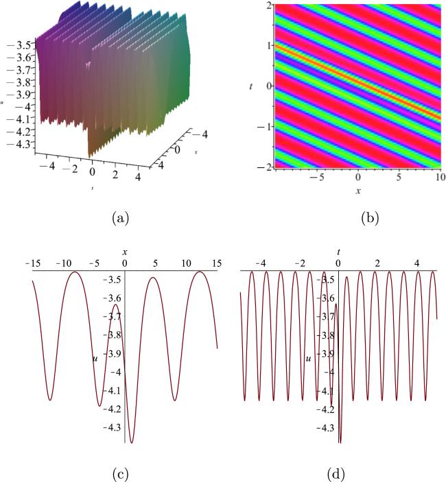
Figure 1 displays the interaction solution u of (86 ) with equations (84 ), (88 ), where the parameters being fixed by equation (90 ), while $v=\tfrac{350251225}{22581504}$ under this selection of parameters.
$\begin{eqnarray}\begin{array}{rcl}{C}_{0} & = & \displaystyle \frac{7}{768},{C}_{1}=\displaystyle \frac{31}{144},{C}_{2}=-\displaystyle \frac{29}{144},{C}_{3}=-\displaystyle \frac{8}{3},\\ {b}_{1} & = & -\displaystyle \frac{5}{6},{c}_{0}=\displaystyle \frac{1}{6},{c}_{1}=-\displaystyle \frac{5}{24},{k}_{0}=\displaystyle \frac{1}{4},{k}_{1}=1,\\ {\omega }_{0} & = & \displaystyle \frac{25045}{8448},{\omega }_{1}=\displaystyle \frac{69635}{6336},p=\displaystyle \frac{1}{2}.\end{array}\end{eqnarray}$
Figure 1. The interaction solution ( |
It can be seen from figure 1 that a solitary wave propagates on background cnoidal waves with a definite speed which can be used to describe relevant phenomena in real nature.
5. Conclusion
In this paper, the DSSH system is investigated by using residual symmetry and the CRE method, respectively. The residual symmetry of the DSSH system is localized into a Lie point symmetry in a prolonged system wherein five new dependent variables are introduced. By applying the classic Lie group method to the prolonged DSSH system, new symmetry reduction solutions are obtained. The DSSH system proves to be CRE integrable and some non-auto Bäcklund transformations of it are derived. In addition, some new interesting interaction solutions between solitons and periodic waves are obtained. We hope that our results will provide some assistance in the study of physical phenomena in shallow water and coastal areas.