


1. Introduction
Realizing fast and efficient quantum population transfer plays an important role in the fields of atomic physics, quantum optics and quantum information [1–5]. Many techniques for quantum population transfer have been proposed in the past decades, and the stimulated Raman adiabatic passage (STIRAP) has become one of the most popular techniques among them [6–9]. The efficient realization of the quantum population transfer for the three-level system from the initial state to the final one can be achieved by employing two partially overlapping delayed laser pulses with a counterintuitive sequence. High transfer efficiency requires the adiabatic condition to be satisfied for the system during the whole process. From the view of experiments, the system needs a large pulse area for the driving pulses, which is equivalent to using a large pulse intensity or spending a very long transfer time [10–12]. Large pulse intensity in experiments may cause damage to the experimental samples or equipment, and a long transfer time duration may exceed the lifetime of the quantum system determined by the decoherence.
The fractional STIRAP (f-STIRAP) is introduced as a modification of the STIRAP technique, allowing for the transfer of a portion of the population from one state to the others in a three-level system. This results in the population existing simultaneously in both of the states at least and the formation of a superposed state [13–19]. The f-STIRAP has the same stability and sensitivity to the external environments as the STIRAP. The population fraction can be achieved by controlling the intensity ratio of the driving pulses at the final time. Reference [20] shows that the adiabatic creation of the maximally coherent superposition is possible even in the absence of the two-photon resonance by chirping the pump and Stokes pulses equally and introducing a chirping delay in the second Stokes pulse for a four-level system. The mechanism has become a powerful tool for producing the superposition states and has been applied to systems such as superconductor qubits [21, 22], ultracold atoms [23, 24], acoustic metamaterials [25] and optical waveguides [26–28]. However, the f-STIRAP still has similar disadvantages to the STIRAP due to the requirement for adiabaticity.
For revolting the adiabatic requirement, several strategies for accelerating the STIRAP have been proposed, including transitionless quantum driving [29–31], fast-forward scaling [32–35], inverse engineering based on the Lewis–Riesenfeld invariants [36, 37], variational method [38, 39], and so on. Some of them are interrelated and can potentially be made equivalent by appropriately adjusting the reference Hamiltonian. Based on their common characteristics, these methods and techniques were also referred to as shortcuts to adiabaticity (STA) [4, 5, 40, 41]. Introducing time-dependent auxiliary pulses to eliminate the system's nonadiabatic couplings, the STA can realize alternative fast processes with the same population of the final state or even the same final state as the STIRAP in a finite short time [42]. It does not require the system to evolve along an adiabatic pathway and has better stability for the parameters of the system, at the cost of applying predesigned auxiliary pulses matched with the transfer process. The applications of the STA have been extended to many classical and quantum systems, such as acoustic waveguides [43], optical waveguides and lattices [44–48], trapped ions [49, 50], quantum dots [51], superconducting circuits [52, 53] and so on. Recently, the related theoretical studies have also been generalized to multilevel systems, including the chainwise and N-pod systems [54–58].
Similar to the relationship between the STA and the STIRAP, the fractional STA (f-SAT) can overcome the shortcomings existing in the f-STIRAP, which needs a high requirement for the adiabatic conditions. The transfer time is shorter than the decoherence time of the system for the f-STA. Despite its superiority, the concept of the f-SAT has never been put forward as far as we know. In this paper, the f-STA is proposed firstly via a three-level system with a Λ-type linkage pattern and a four-level system with a tripod structure and its effectiveness and reliability for the production of the superposition states is verified. The f-STA can transfer the quantum population from one ground state to the others and realize coherent superposition with arbitrary proportion quickly by adjusting the ratio of the coherent pulse intensities. It is shown that the f-STA can bypass the adiabatic requirements, and is more robust than the f-STIRAP by analyzing the effects of the pulse intensity, the time delay and the spontaneous emission on the transfer process.
The present paper is organized as follows. In section 2 , the f-STA of the three-level system for coherently producing the quantum superposition state with the population ratio of $\tfrac{1}{2}:\tfrac{1}{2}$ is proposed, and the effects of the pulse intensity, the time delay and the spontaneous emission on the population transfer are investigated. In section 3 , the f-STA of the four-level system is implemented for achieving a superposed state with a population ratio of $\tfrac{1}{3}:\tfrac{1}{3}:\tfrac{1}{3}$, and the stability of the f-STA under the influence of the pulse intensity, the time delay and the spontaneous emission are discussed. Due to the adjustability of the parameters, the superposition states of any population ratio can be produced by the f-STA in the three- and four-level systems. Multilevel systems, such as N-pod linkage (N ≥ 4), may be reduced into effective three-level systems by the Morris–Shore transformation [59–62]. The mechanism can be generalized to produce the superposition states with more than three states. The conclusion is given in section 4 .
2. Fractional STA for the three-level system
2.1. Theoretical framework
Let us first consider the scheme of the f-STIRAP and the f-STA by a three-level system with a Λ-type linkage pattern, as shown in figure 1. ∣1⟩ and ∣3⟩ correspond to the ground and metastable states, while ∣2⟩ represents the intermediate excited state. The pump pulse ΩP(t) and the Stokes pulse ΩS(t) relate the states ∣1⟩ and ∣3⟩ to the excited state ∣2⟩. In the rotating-wave approximation, the Hamiltonian of the system reads [6–9]
$\begin{eqnarray}{\widehat{H}}_{0}(t)=\displaystyle \frac{{\hslash }}{2}\left(\begin{array}{ccc}0 & {{\rm{\Omega }}}_{{\rm{P}}}(t) & 0\\ {{\rm{\Omega }}}_{{\rm{P}}}(t) & {\rm{\Delta }}(t) & {{\rm{\Omega }}}_{{\rm{S}}}(t)\\ 0 & {{\rm{\Omega }}}_{{\rm{S}}}(t) & 0\end{array}\right).\end{eqnarray}$
The states ∣1⟩ and ∣3⟩ are on two-photon resonance and the state ∣2⟩ is off-resonance from the others by a certain detuning Δ(t). The wavefunction ∣ψ(t)⟩ ≡ c1(t)∣1⟩ + c2(t)∣2⟩ + c3(t)∣3⟩ follows the Schrödinger equation: $\begin{eqnarray}{\rm{i}}{\hslash }\displaystyle \frac{{\rm{d}}}{{\rm{d}}t}| \psi (t)\rangle ={\widehat{H}}_{0}(t)| \psi (t)\rangle .\end{eqnarray}$
Theoretically, the system is only populated on the state ∣1⟩ at the initial time, i.e. c1( − ∞ ) = 1, c2( − ∞ ) = 0 and c3( − ∞ ) = 0, and the dynamics of the system is investigated by monitoring the populations ∣cn( + ∞ )∣2 (n = 1, 2, 3) on all of the states at t → + ∞ .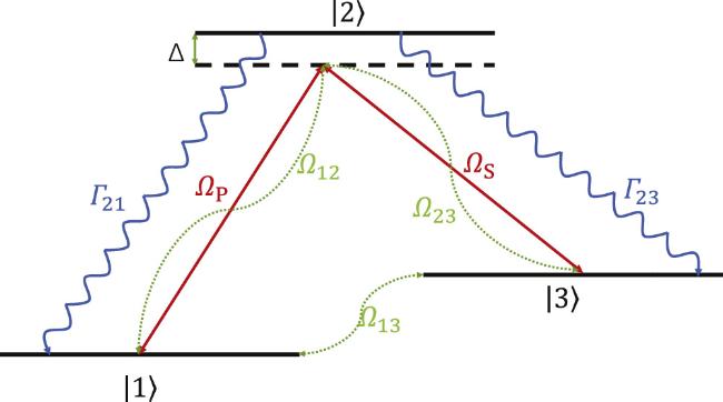
Figure 1. Scheme of the population transfer for the three-level system. The coupling scheme is driven by the pump pulse ΩP and Stokes pulse ΩS (red solid lines) for both of the f-STA and the f-STIRAP. The auxiliary pulses Ω12, Ω23 and Ω13 depicted by the dotted green lines are designed only for the f-STA. Γ21 and Γ23 represent the spontaneous emissions from the intermediate state ∣2⟩ to the states ∣1⟩ and ∣3⟩ (blue wavy lines). |
There are three eigenvalues for the Hamiltonian (1 ): λ0(t) = 0 and ${\lambda }_{\pm }(t)={\hslash }[{\rm{\Delta }}(t)\pm \sqrt{{{\rm{\Delta }}}^{2}(t)+{{\rm{\Omega }}}^{2}(t)}]/2$ with ${\rm{\Omega }}(t)=\sqrt{{{\rm{\Omega }}}_{{\rm{P}}}^{2}(t)+{{\rm{\Omega }}}_{{\rm{S}}}^{2}(t)}$. The dressed eigenstate corresponding to λ0(t) is called the dark state: $| {\lambda }_{0}(t)\rangle \,={\left[\cos \theta (t),0,-\sin \theta (t)\right]}^{{\rm{T}}}$. The dressed eigenstates corresponding to the remaining eigenvalues are called the bright states: $| {\lambda }_{+}(t)\rangle ={\left[\sin \phi (t)\sin \theta (t),\cos \phi (t),\sin \phi (t)\cos \theta (t)\right]}^{{\rm{T}}}$ and $| {\lambda }_{-}(t)\rangle ={\left[\cos \phi (t)\sin \theta (t),-\sin \phi (t),\cos \phi (t)\cos \theta (t)\right]}^{{\rm{T}}}$ with the mixing angles θ(t) and φ(t) defined by $\tan \theta (t)={{\rm{\Omega }}}_{{\rm{P}}}(t)/{{\rm{\Omega }}}_{{\rm{S}}}(t)$ and $\tan 2\phi (t)={\rm{\Omega }}(t)/{\rm{\Delta }}(t)$. The dark state, which is a linear superposition of the pure states ∣1⟩ and ∣3⟩, is used as a passage to produce the coherent superposition state. The proportions are ${\cos }^{2}\theta $ in the state $\left|1\right\rangle $ and ${\sin }^{2}\theta $ in the state $\left|3\right\rangle $ for the whole transfer process. From the representation of the dressed states, the transfer process based on the dark state can be effectively implemented by employing two partially overlapping delayed Gaussian pulses ΩP(t) and ΩS(t) with a counterintuitive sequence. The counter intuition means the Stokes pulse ΩS(t) is opened before the pump pulse ΩP(t). This is the mechanism of the STIRAP [1–3]. For the complete transfer of the populations from $\left|1\right\rangle $ to $\left|3\right\rangle $, the adiabatic condition must be satisfied, which will spend a very long transfer time.
The f-STIRAP can be obtained from the incomplete population transfer of the STIRAP. The variation of the mixing angle during the transfer process is controlled by appropriately designing the pulse sequence. Unlike the STIRAP, here the two pulses vanish simultaneously while maintaining a fixed ratio [14]:
$\begin{eqnarray}\mathop{\mathrm{lim}}\limits_{t\to -\infty }\displaystyle \frac{{{\rm{\Omega }}}_{{\rm{p}}}(t)}{{{\rm{\Omega }}}_{{\rm{S}}}(t)}=0,\quad \mathop{\mathrm{lim}}\limits_{t\to +\infty }\displaystyle \frac{{{\rm{\Omega }}}_{{\rm{p}}}(t)}{{{\rm{\Omega }}}_{{\rm{S}}}(t)}=\tan \alpha .\end{eqnarray}$
The final proportion of the superposition state is determined by the controllable parameter α in the driving pulses. Associated with the definition of the mixing angle θ(t), θ(t → + ∞ ) = α must be obtained. The specific form of the pulses for the f-STIRAP can be designed as follows [14, 18, 19]: $\begin{eqnarray}\begin{array}{rcl}{{\rm{\Omega }}}_{{\rm{P}}}(t) & = & {{\rm{\Omega }}}_{0}\sin \alpha {{\rm{e}}}^{-{\left(t-\tau \right)}^{2}/{T}^{2}},\\ {{\rm{\Omega }}}_{{\rm{S}}}(t) & = & {{\rm{\Omega }}}_{0}[{{\rm{e}}}^{-{\left(t+\tau \right)}^{2}/{T}^{2}}+\cos \alpha {{\rm{e}}}^{-{\left(t-\tau \right)}^{2}/{T}^{2}}].\end{array}\end{eqnarray}$
Ω0 represents the peak pulse intensity, τ represents the time delay between the pump and the Stokes pulses and T represents the common duration of the pulses.The f-STIRAP encounters the drawbacks of requiring a large peak pulse intensity Ω0 and/or longer duration due to the requirement of the adiabatic conditions. In general, it is hard to be realized in realistic platforms. To address this issue, the f-STA is adopted, which introduces the auxiliary pulses to couple the eigenstates, forming a closed loop and eliminating the influence of the nonadiabatic transitions. For obtaining the auxiliary pulses in the STA, the wavefunction $| \tilde{\psi }(t)\rangle =\widehat{U}(t)| \psi (t)\rangle $ follows the time-dependent Schrödinger equation:5 ) [4, 5, 40, 41]. In other words, we need to make ${\widehat{U}}^{\dagger }(t){\widehat{H}}_{a}(t)\widehat{U}(t)-{\rm{i}}{\hslash }{\widehat{U}}^{\dagger }(t)\tfrac{\partial \widehat{U}(t)}{\partial t}=0$, which leads to:
$\begin{eqnarray}{\rm{i}}{\hslash }\displaystyle \frac{\partial | \tilde{\psi }(t)\rangle }{\partial t}=\left[{\widehat{U}}^{\dagger }(t)\widehat{H}(t)\widehat{U}(t)-{\rm{i}}{\hslash }{\widehat{U}}^{\dagger }(t)\displaystyle \frac{\partial \widehat{U}(t)}{\partial t}\right]| \tilde{\psi }(t)\rangle .\end{eqnarray}$
The second term on the right-hand side of the above equation, i.e. ${\rm{i}}{\hslash }{\widehat{U}}^{\dagger }(t)\tfrac{\partial \widehat{U}(t)}{\partial t}$, represents the influence of the nonadiabatic transitions. In order to speed up the production of the superposition states efficiently and robustly, it is necessary to properly induce an auxiliary Hamiltonian ${\widehat{H}}_{a}(t)$, which ensures that only diagonal term ${\widehat{U}}^{\dagger }(t)\widehat{H}(t)\widehat{U}(t)$ exists in the right-hand side of equation ( $\begin{eqnarray}{\widehat{H}}_{a}(t)={\rm{i}}{\hslash }\displaystyle \frac{\partial \widehat{U}(t)}{\partial t}{\widehat{U}}^{\dagger }(t).\end{eqnarray}$
Using the transformation matrix2 ) is substituted by $\widehat{H}(t)={\widehat{H}}_{0}(t)+{\widehat{H}}_{a}(t)$ for implementing the STA. The introduction of the auxiliary pulses allow for the elimination of the nonadiabatic transitions, providing a shortcut to bypass the adiabatic condition [4, 5]. It also avoids the need for large pulse intensities while the production of the superposition states is still robust and efficient. The f-STA originates from the combination of the f-STIRAP and the STA.
$\begin{eqnarray}\widehat{U}(t)=\left(\begin{array}{ccc}\sin \phi (t)\sin \theta (t) & \cos \theta (t) & \cos \phi (t)\sin \theta (t)\\ \cos \phi (t) & 0 & -\sin \phi (t)\\ \sin \phi (t)\cos \theta (t) & -\sin \theta (t) & \cos \phi (t)\cos \theta (t)\end{array}\right),\end{eqnarray}$
the auxiliary Hamiltonian in the three-level system can be derived as $\begin{eqnarray}{\widehat{H}}_{a}(t)={\rm{i}}\left(\begin{array}{ccc}0 & {{\rm{\Omega }}}_{12}(t) & {{\rm{\Omega }}}_{13}(t)\\ -{{\rm{\Omega }}}_{12}(t) & 0 & {{\rm{\Omega }}}_{23}(t)\\ -{{\rm{\Omega }}}_{13}(t) & -{{\rm{\Omega }}}_{23}(t) & 0\end{array}\right),\end{eqnarray}$
with the auxiliary pulses $\begin{eqnarray}\begin{array}{rcl}{{\rm{\Omega }}}_{12}(t) & = & \dot{\phi }(t)\sin \theta (t),{{\rm{\Omega }}}_{23}(t)=-\dot{\phi }(t)\cos \theta (t),\\ {{\rm{\Omega }}}_{13}(t) & = & \dot{\theta }(t).\end{array}\end{eqnarray}$
Here, $\dot{\theta }=({\dot{{\rm{\Omega }}}}_{{\rm{P}}}{{\rm{\Omega }}}_{{\rm{S}}}-{\dot{{\rm{\Omega }}}}_{{\rm{S}}}{{\rm{\Omega }}}_{{\rm{P}}})/{{\rm{\Omega }}}^{2}$ and $\dot{\phi }={\rm{\Delta }}({\dot{{\rm{\Omega }}}}_{{\rm{P}}}{{\rm{\Omega }}}_{{\rm{P}}}\,+{\dot{{\rm{\Omega }}}}_{{\rm{S}}}{{\rm{\Omega }}}_{{\rm{S}}})/[{\rm{\Omega }}({{\rm{\Delta }}}^{2}+4{{\rm{\Omega }}}^{2})]$. The Hamiltonian ${\widehat{H}}_{0}(t)$ in equation (2.2. Coherent production of the superposition state
The population transfer in the f-STIRAP is obtained by directly applying the pulse sequence (4 ) to equations (1 ) and (2 ). The transfer for the f-STA is realized by solving equation (2 ) but the Hamiltonian ${\widehat{H}}_{0}(t)$ is substituted by $\widehat{H}(t)={\widehat{H}}_{0}(t)+{\widehat{H}}_{a}(t)$. The auxiliary Hamiltonian ${\widehat{H}}_{a}(t)$ is provided by equations (8 ) and (9 ). Producing the superposition states with arbitrary proportion are possible but we first examine the most interesting case of equal proportion for the states ∣1⟩ and ∣3⟩. By fixing the parameter α = π/4, the final state can be obtained as $| \psi (+\infty )\rangle =(| 1\rangle -| 3\rangle )/\sqrt{2}$, which corresponds to the population ratio of $\tfrac{1}{2}:\tfrac{1}{2}$ between ∣1⟩ and ∣3⟩. Such a state will be used for example in building Raman qubit gates for quantum computation [63, 64].
The evolution of the populations for the f-STA and the f-STIRAP via the dark-state passage ∣λ0(t)⟩ is demonstrated in figures 2(a) and (b), respectively. The population is assumed to stay on state ∣1⟩ at the initial time, and then 50% of it is transferred to state ∣3⟩ at the final time for the f-STA in figure 2(a). There is no population in the state ∣2⟩ during the whole process. By contrast, the final population on ∣3⟩ does not reach 0.5 for the f-STIRAP in figure 2(b), because there is some population loss due to the nonadiabatic transitions. The f-STA introduces three auxiliary pulses (9 ) to eliminate the nonadiabatic transitions, perfectly achieving a coherent superposition state of ∣1⟩ and ∣3⟩ with equal proportion. Figure 2(c) shows the effect of the peak pulse intensity Ω0 on the population transfer. The final population on ∣3⟩ for the f-STA does not change with Ω0 and always keeps at 0.5 for the f-STA. The transfer is not sensitive to the change of the pulse intensity. However, the final population on ∣3⟩ for the f-STIRAP increases rapidly with increasing the pulse intensity first, then drops to 0.5 after reaching a peak, and finally oscillates around 0.5 with the characteristic of amplitude attenuation. Obviously, the transfer for the f-STIRAP is affected dramatically by the change in the pulse intensity. Figure 2(d) shows the effect of the time delay τ on the population transfer. The final population on ∣3⟩ for the f-STA increases rapidly with increasing τ and reaches 0.5 during a small time delay. For the larger time delay, the population always stays at 0.5. This means the presence of the three auxiliary pulses lessens the requirement that the two driving pulses must overlap. The final population on ∣3⟩ for the f-STIRAP increases with increasing the value of τ, but the growth of the population is relatively slow, and 50% of the population can be achieved only at τ ≈ 0.47T. With increasing the time delay, the population on ∣3⟩ continues to rise and stabilizes after reaching to about 0.86. As the time delay is increased, the overlap between the two driving pulses becomes smaller and smaller. Eventually, the two pulses no longer overlap, leading to a situation where the adiabatic condition is not satisfied. Consequently, the f-STIRAP cannot give reliable results for a larger time delay.
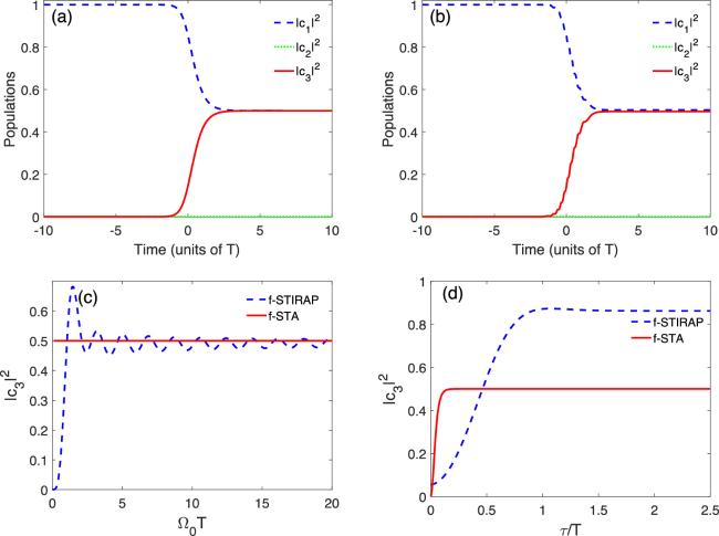
Figure 2. Population transfer in the three-level system via the dark-state passage for the f-STA in (a) and for the f-STIRAP in (b). The parameters are chosen as α = π/4, Ω0T = 2.0, τ/T = 0.7 and Δ = 0.2π. The effects of the peak pulse intensity Ω0 in (c) at τ = 0.7T and the time delay τ in (d) at Ω0T = 2.0 on the final population on ∣3⟩ for both of the f-STA (red solid line) and the f-STIRAP (blue dashed line). |
The parameter α in the driving pulses is pivotal for the production of the superposition states. The change of the final population on ∣3⟩ with α is given in figure 3. According to equation (3 ), the population on the state ∣3⟩ changes with α as the form of ${\sin }^{2}\alpha $ at the final time, which is confirmed numerically by the red solid line for the f-STA in figure 3. The conversion rate of 0.5 can be obtained once α = π/4 or 3π/4 is chosen. By comparison, the change of the population on ∣3⟩ with α for the f-STIRAP (blue dashed line) deviates from the analytic result. The amplitude and periodic of the oscillation are further reduced. To demonstrate the controllability, the superposition state with an unequal population is investigated. As an example, the superposition state with the final population ratio of $\tfrac{1}{3}:\tfrac{2}{3}$ between the states ∣1⟩ and ∣3⟩ is shown in figure 4 by choosing the parameter $\alpha =\arccos (1/\sqrt{3})$. It is shown that the population ratio for the f-STA can be controlled precisely, but not for the f-STIRAP. The production of the coherent states by the f-STA is more robust than that by the f-STIRAP under the same parameter condition.
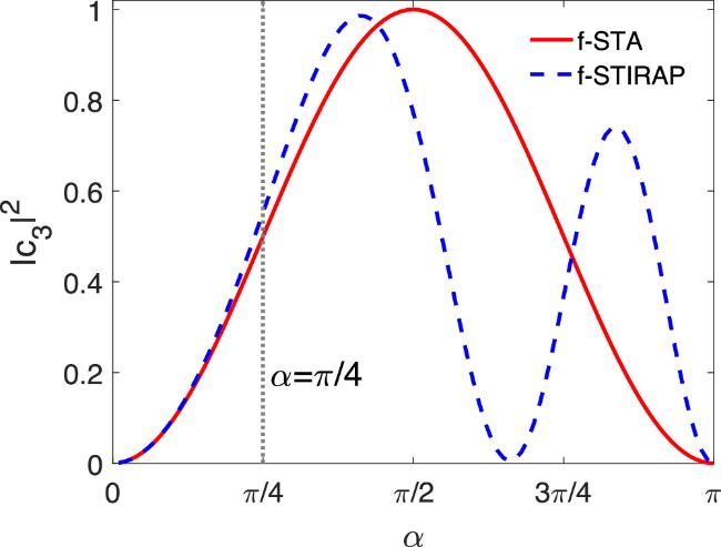
Figure 3. Change of the final population on ∣3⟩ with the parameter α for the f-STA (red solid line) and the f-STIRAP (blue dashed line). The vertical dotted line corresponds to α = π/4. The other parameters are chosen as Ω0T = 2.0, τ/T = 0.7 and Δ = 0.2π. |
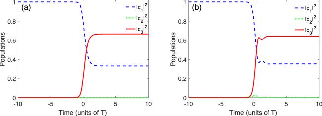
Figure 4. Population transfer in the three-level system via the dark-state passage for the f-STA in (a) and for the f-STIRAP in (b). The control parameter is chosen as $\alpha =\arccos (1/\sqrt{3})$, and the other parameters are the same as that in figures 2(a) and (b). |
2.3. Effect of the spontaneous emission
In the realistic process of preparing the coherent superposition states, the presence of the spontaneous emission in the excited state is inevitable. To obtain the transfer efficiency of the f-STA and the f-STIRAP under the influence of spontaneous emission, the density matrix based on the quantum master equation is used to describe the change of the population in each energy level of the system. The dynamic evolution of the density operator for the system is described by [65–67]:10 ), the Lindblad term for the three-level system is concretely written as:
$\begin{eqnarray}\begin{array}{rcl}{\rm{i}}{\hslash }\dot{\hat{\rho }} & = & [\widehat{H}(t),\hat{\rho }]+\widehat{D}[\hat{\rho }],\\ \widehat{D}[\hat{\rho }] & = & \displaystyle \sum _{i}{\gamma }_{i}(2{\hat{L}}_{i}\hat{\rho }{\hat{L}}_{i}^{\dagger }-{\hat{L}}_{i}^{\dagger }{\hat{L}}_{i}\hat{\rho }-\hat{\rho }{\hat{L}}_{i}^{\dagger }{\hat{L}}_{i}).\end{array}\end{eqnarray}$
$\widehat{D}[\hat{\rho }]$ represents the Lindblad term related to the spontaneous emission in the excited state, which is composed of the spontaneous emission rate γi (i = 1, 2) and the jump operators ${\hat{L}}_{1}=\left|1\right\rangle \left\langle 2\right|$ and ${\hat{L}}_{2}=\left|3\right\rangle \left\langle 2\right|$. The spontaneous emission from the state $\left|2\right\rangle $ to the states $\left|1\right\rangle $ and $\left|3\right\rangle $ in the three-level system are denoted by γ1 = iΓ21 and γ2 = iΓ23, respectively. According to equation ( $\begin{eqnarray}\begin{array}{l}\widehat{D}[\hat{\rho }]\\ \ \ =\,-\displaystyle \frac{{\rm{i}}{\hslash }}{2}\left(\begin{array}{ccc}-2{{\rm{\Gamma }}}_{21}{\rho }_{22} & ({{\rm{\Gamma }}}_{21}+{{\rm{\Gamma }}}_{23}){\rho }_{12} & 0\\ ({{\rm{\Gamma }}}_{21}+{{\rm{\Gamma }}}_{23}){\rho }_{21} & 2({{\rm{\Gamma }}}_{21}+{{\rm{\Gamma }}}_{23}){\rho }_{22} & ({{\rm{\Gamma }}}_{21}+{{\rm{\Gamma }}}_{23}){\rho }_{23}\\ 0 & ({{\rm{\Gamma }}}_{21}+{{\rm{\Gamma }}}_{23}){\rho }_{32} & -2{{\rm{\Gamma }}}_{23}{\rho }_{22}\end{array}\right).\end{array}\end{eqnarray}$
To simplify the calculation, Γ21 = Γ23 ≡ Γ is taken, and the dimensionless spontaneous emission rate γ = ΓT is introduced. The change of the components ρ11, ρ22, and ρ33 for the density operator with γ by solving equation (10 ) is demonstrated in figure 5. Figure 5(a) illustrates the case for the f-STA. ρ11 and ρ33 always stay at 0.5, which is independent of the spontaneous emission. The reason is that the population in the excited state is always zero, so the spontaneous emission does not work for the transfer. Figure 5(b) shows the case for the f-STIRAP. ρ11 increases and ρ33 decreases gradually with increasing γ for the f-STIRAP. Population transfer is suppressed by the spontaneous emission rate in this situation. In the process of dynamical evolution, the spontaneous emission of the population in the excited state ∣2⟩ to the state ∣1⟩ is more significant than to the state ∣3⟩ for a larger emission rate. The changes in the population with the spontaneous emission under the counterintuitive pulse sequence for the f-STIRAP and the f-STA are very different. It is evident that the f-STA is more advantageous than the f-STIRAP for preparing the coherent superposition with two states in the open systems.
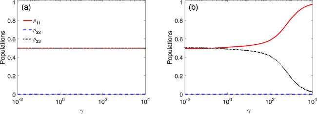
Figure 5. Change of the final populations ρ11, ρ22 and ρ33 with the spontaneous emission rate γ. (a) The case for the f-STA and (b) the case for the f-STIRAP. The other parameters are chosen as α = π/4, Ω0T = 2.0, τ/T = 0.7 and Δ = 0.2π. |
3. Fractional STA for the four-level system
3.1. Theoretical framework
The scheme for the f-STIRAP and the f-STA in the four-level system with a tripod linkage pattern is shown in figure 6. The Hamiltonian in the rotating-wave approximation is written as [3, 15]2 ) but with the probability amplitude $c(t)={\left[{c}_{1}(t),{c}_{2}(t),{c}_{3}(t),{c}_{4}(t)\right]}^{{\rm{T}}}$. The system is only populated on the state ∣1⟩ at the initial time, i.e. c1( − ∞ ) = 1, c2( − ∞ ) = 0, c3( − ∞ ) = 0 and c4( − ∞ ) = 0, and the dynamics of the system is investigated by monitoring the populations ∣cn( + ∞ )∣2 (n = 1, 2, 3, 4) at t → + ∞ .
$\begin{eqnarray}{\widehat{H}}_{0}(t)=\displaystyle \frac{{\hslash }}{2}\left(\begin{array}{cccc}0 & {{\rm{\Omega }}}_{{\rm{P}}}(t) & 0 & 0\\ {{\rm{\Omega }}}_{{\rm{P}}}(t) & {\rm{\Delta }} & \,{{\rm{\Omega }}}_{{\rm{S}}}(t) & {{\rm{\Omega }}}_{{\rm{Q}}}(t)\\ 0 & {{\rm{\Omega }}}_{{\rm{S}}}(t) & 0 & 0\\ 0 & {{\rm{\Omega }}}_{{\rm{Q}}}(t) & 0 & 0\end{array}\right),\end{eqnarray}$
where ΩP(S,Q)(t) represents the driving pulses between the pure states ∣2⟩ and ∣1⟩ (∣3⟩, ∣4⟩). Similar to the three-level system, here the pure states follow equation (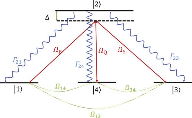
Figure 6. Scheme of the population transfer for the four-level system. The coupling scheme is realized by the pump pusle ΩP and the Stokes pulses ΩQ and ΩS (red solid lines) for the f-STA and the f-STIRAP. The auxiliary pulses Ω13, Ω14 and Ω34 depicted by the dotted green lines are designed only for the f-STA. Γ21, Γ23 and Γ24 represent the spontaneous emissions from the intermediate state ∣2⟩ to the initial state ∣1⟩ and the two final states ∣3⟩ and ∣4⟩ (blue wavy lines). |
The eigenvalues of the Hamiltonian (12 ) are ED1 = ED2 = 0, ${E}_{B1}={\hslash }[{\rm{\Delta }}(t)+\sqrt{{{\rm{\Delta }}}^{2}(t)+{{\rm{\Omega }}}^{2}(t)}]/2$ and ${E}_{B2}={\hslash }[{\rm{\Delta }}(t)\,-\sqrt{{{\rm{\Delta }}}^{2}(t)+{{\rm{\Omega }}}^{2}(t)}]/2$ with ${\rm{\Omega }}(t)=\sqrt{{{\rm{\Omega }}}_{{\rm{P}}}^{2}(t)+{{\rm{\Omega }}}_{{\rm{S}}}^{2}(t)+{{\rm{\Omega }}}_{{\rm{Q}}}^{2}(t)}$. Accordingly, there are four dressed eigenstates, with two being dark states and two being bright states:
$\begin{eqnarray}\begin{array}{rcl}| {E}_{D1}(t)\rangle & = & \left(\begin{array}{c}\cos \theta (t)\\ 0\\ -\sin \theta (t)\cos \eta (t)\\ -\sin \theta (t)\sin \eta (t)\end{array}\right),\\ | {E}_{D2}(t)\rangle & = & \left(\begin{array}{c}0\\ 0\\ \sin \eta (t)\\ -\cos \eta (t)\end{array}\right),\\ | {E}_{B1}(t)\rangle & = & \left(\begin{array}{c}\sin \phi (t)\sin \theta (t)\\ \cos \phi (t)\\ \sin \phi (t)\cos \theta (t)\cos \eta (t)\\ \sin \phi (t)\cos \theta (t)\sin \eta (t)\end{array}\right),\\ | {E}_{B2}(t)\rangle & = & \left(\begin{array}{c}\cos \phi (t)\sin \theta (t)\\ -\sin \phi (t)\\ \cos \phi (t)\cos \theta (t)\cos \eta (t)\\ \cos \phi (t)\cos \theta (t)\sin \eta (t)\end{array}\right).\end{array}\end{eqnarray}$
The mixing angles are determined by $\tan \eta (t)\,={{\rm{\Omega }}}_{{\rm{Q}}}(t)/{{\rm{\Omega }}}_{{\rm{S}}}(t)$, $\tan \theta (t)={{\rm{\Omega }}}_{{\rm{P}}}(t)/\sqrt{{{\rm{\Omega }}}_{{\rm{S}}}^{2}(t)+{{\rm{\Omega }}}_{{\rm{Q}}}^{2}(t)}$ and $\phi \,=\arctan (\sqrt{{{\rm{\Omega }}}_{{\rm{P}}}^{2}(t)+{{\rm{\Omega }}}_{{\rm{S}}}^{2}(t)+{{\rm{\Omega }}}_{{\rm{Q}}}^{2}(t)}/{\rm{\Delta }})/2$. When the system is in the dark state ∣ED1(t)⟩, the superposition of $\left|1\right\rangle $, $\left|3\right\rangle $, and $\left|4\right\rangle $ with arbitrary proportion can be determined by the mixing angles θ and η. The proportion will be ${\cos }^{2}\theta $ in the state $\left|1\right\rangle $, ${\sin }^{2}\theta {\cos }^{2}\eta $ in the state $\left|3\right\rangle $, and ${\sin }^{2}\theta {\sin }^{2}\eta $ in the state $\left|4\right\rangle $ for the whole process. The specific form of the driving pulses for the four-level system is chosen as $\begin{eqnarray}\begin{array}{rcl}{{\rm{\Omega }}}_{{\rm{P}}}(t) & = & {{\rm{\Omega }}}_{0}\sin \beta {{\rm{e}}}^{-{\left(t-\tau \right)}^{2}/{T}^{2}},\\ {{\rm{\Omega }}}_{{\rm{S}}}(t) & = & {{\rm{\Omega }}}_{0}[{{\rm{e}}}^{-{\left(t+\tau \right)}^{2}/{T}^{2}}+\cos \beta \cos \chi {{\rm{e}}}^{-{\left(t-\tau \right)}^{2}/{T}^{2}}],\\ {{\rm{\Omega }}}_{{\rm{Q}}}(t) & = & {{\rm{\Omega }}}_{0}[{{\rm{e}}}^{-{\left(t+\tau \right)}^{2}/{T}^{2}}+\cos \beta \sin \chi {{\rm{e}}}^{-{\left(t-\tau \right)}^{2}/{T}^{2}}].\end{array}\end{eqnarray}$
The final proportion of the superposition state is determined by the controllable parameters β and χ in the pulses. Associated with the definition of the mixing angles, we have θ(t → + ∞ ) = β and η(t → + ∞ ) = χ.Now, we will demonstrate the process for obtaining the auxiliary pulses for implementing the f-STA in the four-level system. Based on equation (13 ), the unitary transformation matrix of the four-level system is constructed as6 ) is
$\begin{eqnarray}\widehat{U}(t)=\left(\begin{array}{cccc}\cos \theta (t) & 0 & \sin \phi (t)\sin \theta (t) & \cos \phi (t)\sin \theta (t)\\ 0 & 0 & \cos \phi (t) & -\sin \phi (t)\\ -\sin \theta (t)\cos \eta (t) & \sin \eta (t) & \sin \phi (t)\cos \theta (t)\cos \eta (t) & \cos \phi (t)\cos \theta (t)\cos \eta (t)\\ -\sin \theta (t)\sin \eta (t) & -\cos \eta (t) & \sin \phi (t)\cos \theta (t)\sin \eta (t) & \cos \phi (t)\cos \theta (t)\sin \eta (t)\end{array}\right).\end{eqnarray}$
The auxiliary Hamiltonian according to equation ( $\begin{eqnarray}{\widehat{H}}_{a}={\rm{i}}\left(\begin{array}{cccc}0 & {{\rm{\Omega }}}_{12}(t) & {{\rm{\Omega }}}_{13}(t) & {{\rm{\Omega }}}_{14}(t)\\ -{{\rm{\Omega }}}_{12}(t) & 0 & {{\rm{\Omega }}}_{23}(t) & {{\rm{\Omega }}}_{24}(t)\\ -{{\rm{\Omega }}}_{13}(t) & -{{\rm{\Omega }}}_{23}(t) & 0 & {{\rm{\Omega }}}_{34}(t)\\ -{{\rm{\Omega }}}_{14}(t) & -{{\rm{\Omega }}}_{24}(t) & -{{\rm{\Omega }}}_{34}(t) & 0\end{array}\right),\end{eqnarray}$
and the specific forms of the auxiliary pulses are $\begin{eqnarray}\begin{array}{rcl}{{\rm{\Omega }}}_{12}(t) & = & \dot{\phi }(t)\sin \theta (t),{{\rm{\Omega }}}_{13}(t)=\dot{\theta }(t)\cos \eta (t),\\ {{\rm{\Omega }}}_{14}(t) & = & \dot{\theta }(t)\sin \eta (t),\\ {{\rm{\Omega }}}_{23}(t) & = & -\dot{\phi }(t)\cos \theta (t)\cos \eta (t),\\ {{\rm{\Omega }}}_{24}(t) & = & -\dot{\phi }(t)\cos \theta (t)\sin \eta (t),{{\rm{\Omega }}}_{34}(t)=-\dot{\eta }(t),\end{array}\end{eqnarray}$
with $\dot{\theta }=[{\dot{{\rm{\Omega }}}}_{{\rm{P}}}({{\rm{\Omega }}}_{{\rm{S}}}^{2}+{{\rm{\Omega }}}_{{\rm{Q}}}^{2})-{{\rm{\Omega }}}_{{\rm{p}}}({{\rm{\Omega }}}_{{\rm{S}}}{\dot{{\rm{\Omega }}}}_{{\rm{S}}}+{{\rm{\Omega }}}_{{\rm{Q}}}{\dot{{\rm{\Omega }}}}_{{\rm{Q}}})]/[({{\rm{\Omega }}}_{{\rm{S}}}^{2}+{{\rm{\Omega }}}_{{\rm{Q}}}^{2}+{{\rm{\Omega }}}_{{\rm{P}}}^{2})\sqrt{{{\rm{\Omega }}}_{{\rm{S}}}^{2}+{{\rm{\Omega }}}_{{\rm{Q}}}^{2}}]$, $\dot{\eta }=({\dot{{\rm{\Omega }}}}_{{\rm{Q}}}{{\rm{\Omega }}}_{{\rm{S}}}-{\dot{{\rm{\Omega }}}}_{{\rm{S}}}{{\rm{\Omega }}}_{{\rm{Q}}})/({{\rm{\Omega }}}_{{\rm{S}}}^{2}+{{\rm{\Omega }}}_{{\rm{Q}}}^{2})$, and $\dot{\phi }={\rm{\Delta }}({\dot{{\rm{\Omega }}}}_{{\rm{P}}}{{\rm{\Omega }}}_{{\rm{P}}}+{\dot{{\rm{\Omega }}}}_{{\rm{S}}}{{\rm{\Omega }}}_{{\rm{S}}}+{\dot{{\rm{\Omega }}}}_{{\rm{Q}}}{{\rm{\Omega }}}_{{\rm{Q}}})/[{\rm{\Omega }}({{\rm{\Delta }}}^{2}+4{{\rm{\Omega }}}^{2})]$. Because ∣ED1(t)⟩ and ∣ED2(t)⟩ are degenerate, the nonadiabatic coupling between them cannot be suppressed, even in the adiabatic limit. The nonadiabatic coupling between ∣ED1(t)⟩ and ∣ED2(t)⟩ causes a transition between them with probability ${\sin }^{2}[{\int }_{-\infty }^{+\infty }\dot{\eta }(t)\sin \theta (t){\rm{d}}t]$ [15]. When the mixing angle η(t) is chosen time-independent, there is no any transition between them. The population transfer of the system will only keep in the dark-state passage given by ∣ED1(t)⟩. The superposition of the states $\left|1\right\rangle $, $\left|3\right\rangle $ and $\left|4\right\rangle $ with arbitrary proportion can be realized by choosing suitable θ and η.3.2. Coherent production of the superposition state
We first demonstrate the case of the superposition of the states $\left|1\right\rangle $, $\left|3\right\rangle $ and $\left|4\right\rangle $ with equal proportion. The final state is $\left|\psi (+\infty )\right\rangle =(\left|1\right\rangle +\left|3\right\rangle +\left|4\right\rangle )/\sqrt{3}$ and the ratio of the populations on $\left|1\right\rangle $, $\left|3\right\rangle $ and $\left|4\right\rangle $ is $\tfrac{1}{3}:\tfrac{1}{3}:\tfrac{1}{3}$. The controllable parameters $\beta =\arccos (1/\sqrt{3})$ and χ = π/4 are selected for realizing the equal superposition of the three low-energy states. This superposition state is useful for building three-bit quantum gates for quantum computation [63, 64].
The evolution of the populations in the four-level system via the dark-state passage ∣ED1(t)⟩ is demonstrated in figures 7(a) and (b). Figure 7(a) illustrates the population transfer for the f-STA from the initial state ∣1⟩ to the two final ones ∣3⟩ and ∣4⟩. The population is on state ∣1⟩ at the initial time, and then 1/3 of it is transferred to state ∣3⟩ and 1/3 to ∣4⟩ at the final time. There is no population on ∣2⟩ during the whole process. The final populations on ∣3⟩ and ∣4⟩ do not reach 1/3 for the f-STIRAP in figure 7(b). The f-STA introduces a group of auxiliary pulses (17 ) to eliminate the nonadiabatic transitions, perfectly achieving a coherent superposition state of ∣1⟩, ∣3⟩ and ∣4⟩ with equal proportion.
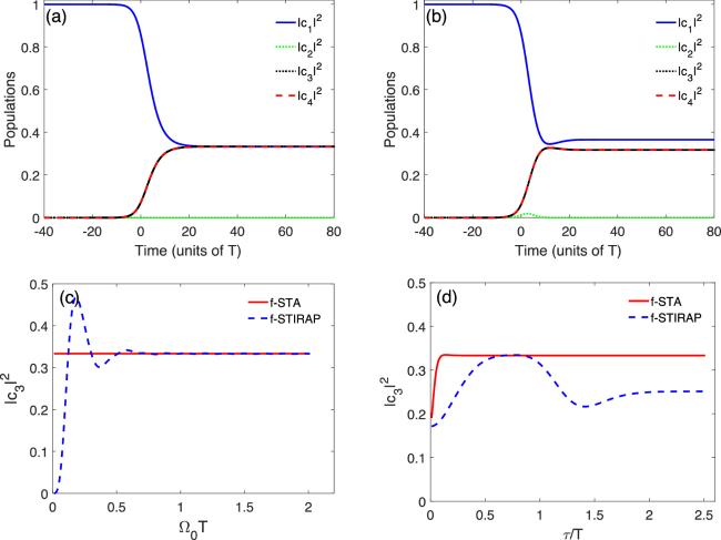
Figure 7. Population transfer in the four-level system by the dark-state passage for the f-STA in (a) and for the f-STIRAP in (b). The parameters are chosen as $\beta =\arccos (1/\sqrt{3})$, χ = π/4, Ω0T = 2.0, τ/T = 0.7 and Δ = 0.2π. The effects of the peak pulse intensity Ω0 in (c) at τ/T = 0.7 and the time delay τ in (d) at Ω0T = 2.0 on the population of the state ∣3⟩ for both of the f-STA (red solid line) and the f-STIRAP (blue dashed line). |
The effects of the peak pulse intensity and the time delay on the final populations are illustrated in figures 7(c) and (d). Figure 7(c) shows the change of the final population on $\left|3\right\rangle $ with the peak pulse intensity Ω0. The final population on $\left|3\right\rangle $ with Ω0 for the f-STIRAP exhibits oscillation around 1/3. The amplitude of such oscillation decreases with further increasing the pulse intensity. By comparison, due to bypassing the adiabatic requirement by the auxiliary pulses, the f-STA consistently achieves a transfer efficiency of 1/3 regardless of the magnitude of the pulse intensity. Figure 7(d) shows the change of the final population on $\left|3\right\rangle $ with the time delay τ. The final population on $\left|3\right\rangle $ is increased to 1/3 for the f-STA when the time delay is larger than a small critical value. For an even larger time delay, the population keeps at 1/3 and is independent of τ. The population transfer can be accomplished even if the driving pulses do not overlap due to the presence of the auxiliary pulses. The population on $\left|3\right\rangle $ for the f-STIRAP approaches about 1/3 when τ is at a small range near 0.7T. The population deviates largely from 1/3 for the other part of the time delay. The population on $\left|4\right\rangle $ changes synchronously with that on $\left|3\right\rangle $ for the chosen parameter χ = π/4, so the corresponding results have not been shown.
Unlike the three-level system, there are two controllable parameters β and χ in the driving pulses for the four-level system in order to produce the superposition states. The changes of the final populations on $\left|1\right\rangle $, $\left|3\right\rangle $ and $\left|4\right\rangle $ with β are demonstrated in figures 8(a), (b) and (c). For χ = π/4, the theoretical populations are ${\cos }^{2}\beta $ on $\left|1\right\rangle $ and ${\sin }^{2}\beta /2$ on $\left|3\right\rangle $ and $\left|4\right\rangle $ since θ(t → + ∞ ) = β is taken. It is found that the final populations for the f-STA and the f-STIRAP are consistent with the theoretical values when β is within the range of 0 to π/2. When β is in the range of π/2 to π, the results for both the f-STA and the f-STIRAP deviate from the theoretical values. The change of the final populations on $\left|1\right\rangle $, $\left|3\right\rangle $ and $\left|4\right\rangle $ with χ is demonstrated in figures 8(d), (e) and (f). For $\beta =\arccos (1/\sqrt{3})$, the theoretical populations are 1/3 on $\left|1\right\rangle $, $(2{\cos }^{2}\chi )/3$ on $\left|3\right\rangle $ and $(2{\sin }^{2}\chi )/3$ on $\left|4\right\rangle $. When the parameter χ is chosen at the range of 0 to π/2, the change of the populations with χ for the f-STA agrees with the theoretical value, while the population for the f-STIRAP does not align with the theoretical value. When the parameter χ is in the range of π/2 to π, the populations for the f-STA and the f-STIRAP no longer fully agree with the theoretical value. When the two parameters are selected in the range of 0 to π/2, the f-STA can achieve any proportional superposition of $\left|1\right\rangle $, $\left|3\right\rangle $ and $\left|4\right\rangle $, but the f-STIRAP cannot do that. As an example, the superposition state with the final population ratio of $\tfrac{1}{6}:\tfrac{1}{3}:\tfrac{1}{2}$ between the states ∣1⟩, ∣3⟩ and ∣4⟩ is shown in figure 9 by choosing the parameters $\beta =\arccos (1/\sqrt{6})$ and $\chi =\arccos (\sqrt{2/5})$. This fully demonstrates the stability and controllability of the f-STA in the realization of the superposition states with three components.

Figure 8. Change of the final populations on ∣1⟩, ∣3⟩ and ∣4⟩ with β in (a)–(c) and χ in (d)–(f) for the f-STA (red solid line) and the f-STIRAP (blue dashed line). The dotted–dashed lines give the corresponding theoretical results. The vertical dotted line corresponds to $\beta =\arccos (1/\sqrt{3})$ in (a-c) and χ = π/4 in (d)–(f), respectively. The other parameters are chosen as Ω0T = 2.0, τ/T = 0.7 and Δ = 0.2π. |
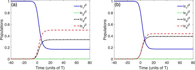
Figure 9. Population transfer in the four-level system by the dark-state passage for the f-STA in (a) and for the f-STIRAP in (b). The control parameters are chosen as $\beta =\arccos (1/\sqrt{6})$ and $\chi =\arccos (\sqrt{2/5})$. The other parameters are same with that in figures 7(a) and (b). |
3.3. Effect of the spontaneous emission
When the spontaneous emission is considered, the population transfer can be investigated by solving the quantum master equation (10 ) of the density operators. For the four-level system, the spontaneous emissions from the state $\left|2\right\rangle $ to the other states are denoted as γi (i = 1, 2, 3), where γ1 = iΓ21, γ2 = iΓ23 and γ3 = iΓ24. The jump operators are defined as ${\hat{L}}_{1}=\left|1\right\rangle \left\langle 2\right|$, ${\hat{L}}_{2}=\left|3\right\rangle \left\langle 2\right|$ and ${\hat{L}}_{3}=\left|4\right\rangle \left\langle 2\right|$. According to equation (10 ), the following Lindblad term can be expressed as:
$\begin{eqnarray}\widehat{D}[\hat{\rho }]=-\displaystyle \frac{{\rm{i}}{\hslash }}{2}\left(\begin{array}{cccc}-2{{\rm{\Gamma }}}_{21}{\rho }_{22} & \left({{\rm{\Gamma }}}_{21}+{{\rm{\Gamma }}}_{23}+{{\rm{\Gamma }}}_{24}\right){\rho }_{12} & 0 & 0\\ \left({{\rm{\Gamma }}}_{21}+{{\rm{\Gamma }}}_{23}+{{\rm{\Gamma }}}_{24}\right){\rho }_{21} & 2\left({{\rm{\Gamma }}}_{21}+{{\rm{\Gamma }}}_{23}+{{\rm{\Gamma }}}_{24}\right){\rho }_{22} & \left({{\rm{\Gamma }}}_{21}+{{\rm{\Gamma }}}_{23}+{{\rm{\Gamma }}}_{24}\right){\rho }_{23} & \left({{\rm{\Gamma }}}_{21}+{{\rm{\Gamma }}}_{23}+{{\rm{\Gamma }}}_{24}\right){\rho }_{24}\\ 0 & \left({{\rm{\Gamma }}}_{21}+{{\rm{\Gamma }}}_{23}+{{\rm{\Gamma }}}_{24}\right){\rho }_{32} & -2{{\rm{\Gamma }}}_{23}{\rho }_{22} & 0\\ 0 & \left({{\rm{\Gamma }}}_{21}+{{\rm{\Gamma }}}_{23}+{{\rm{\Gamma }}}_{24}\right){\rho }_{42} & 0 & -2{{\rm{\Gamma }}}_{24}{\rho }_{22}\end{array}\right).\end{eqnarray}$
It is supposed that Γ21 = Γ23 = Γ24 ≡ Γ is satisfied and γ = ΓT represents the dimensionless spontaneous emission rate.The effect of the spontaneous emission on the population transfer for the four-level system is shown in figure 10. Figure 10(a) illustrates the change of the populations with the spontaneous emission rate γ for the f-STA. The components of the density operator ρ11, ρ33 and ρ44 always keep at 1/3, which is independent of the spontaneous emission. There is no population on ρ22 during the whole transfer process. Figure 10(b) illustrates the change of the populations with γ for the f-STIRAP. When the spontaneous emission rate is sufficiently small, the population on the components ρ11, ρ33 and ρ44 almost is 1/3. The mechanism of the f-STIRAP plays a key role. For even larger γ (overdamping), the population is dominated by spontaneous emission. The transfer process is suppressed and the population mainly stays on the state $\left|1\right\rangle $. For the intermediate value of the spontaneous emission rate (γ ∼ 1), there exists some competition between the f-STIRAP and the spontaneous emission. The f-STA is more advantageous than the f-STIRAP for preparing coherent superposition with three states in the open systems.

Figure 10. Change of the final populations ρ11, ρ22, ρ33 and ρ44 with the spontaneous emission rate γ: (a) the case for the f-STA and (b) the case for the f-STIRAP. The other parameters are chosen as $\beta =\arccos (1/\sqrt{3})$, χ = π/4, Ω0T = 2.0, τ/T = 0.7 and Δ = 0.2π. |
4. Conclusions
The scheme for realizing the coherent superposition states in a three-level system and a four-level system by the f-STA is proposed. For the three-level system with the Λ-type linkage pattern, the superposition state can be implemented by an auxiliary Hamiltonian, which is determined by the two driving pulses with a specific value of the controllable parameter α. For the four-level system with a tripod structure, the superposition states can be realized by another auxiliary Hamiltonian, which can be derived by designing three suitable driving pulses with specific values of the two controllable parameters β and χ. The effects of the peak pulse intensity and the time delay of the driving pulses on the population transfer are studied by solving the time-dependent Schrödinger equations. Compared to the f-STIRAP, the transfer process for the f-STA is not limited by the requirement for the adiabaticity of the system. The effectiveness of utilizing the f-STA to prepare two- and three-state superpositions in the three- and four-level systems is investigated, taking into account the influence of the spontaneous emission from the intermediate state. The spontaneous emission has a suppressive effect on the preparation of the superposition states in the f-STIRAP, but it has little impact on the f-STA. The f-STA allows for the realization of arbitrary proportions of superposition states by controlling the parameters of the driving pulses. The fast and robust production of the superposition states by the f-STA is verified and the mechanism can be generalized to produce the superposition states with more than three components in the future.