Welcome to visit Communications in Theoretical Physics,
Mathematical Physics

Multi-component decompositions, linear superpositions, and new nonlinear integrable coupled KdV-type systems

  • Xiazhi Hao 1 ,
  • S Y Lou , 2, *
Expand
  • 1School of Mathematical Science, Zhejiang University of Technology, Hangzhou 310014, China
  • 2School of Physical Science and Technology, Ningbo University, Ningbo 315211, China

*Author to whom any correspondence should be addressed.

Received date: 2024-08-07

  Revised date: 2024-09-14

  Accepted date: 2024-10-09

  Online published: 2024-11-15

Copyright

© 2024 Institute of Theoretical Physics CAS, Chinese Physical Society and IOP Publishing. All rights, including for text and data mining, AI training, and similar technologies, are reserved.

Abstract

In the realm of nonlinear integrable systems, the presence of decompositions facilitates the establishment of linear superposition solutions and the derivation of novel coupled systems exhibiting nonlinear integrability. By focusing on single-component decompositions within the potential BKP hierarchy, it has been observed that specific linear superpositions of decomposition solutions remain consistent with the underlying equations. Moreover, through the implementation of multi-component decompositions within the potential BKP hierarchy, successful endeavors have been undertaken to formulate linear superposition solutions and novel coupled KdV-type systems that resist decoupling via alterations in dependent variables.

Cite this article

Xiazhi Hao , S Y Lou . Multi-component decompositions, linear superpositions, and new nonlinear integrable coupled KdV-type systems[J]. Communications in Theoretical Physics, 2025 , 77(2) : 025001 . DOI: 10.1088/1572-9494/ad84bd

1. Introduction

A prevalent approach for addressing high-dimensional nonlinear partial differential equations (PDEs) involves decomposing these equations into multiple low-dimensional counterparts, thereby facilitating their treatment using available computational tools [1, 2]. In our investigations, we focused on specific classes of PDEs, namely the potential B-type Kadomtsev–Petviashvili (pBKP) equations derived from the standard KP hierarchy through the imposition of an additional condition between the Lax operator and its adjoint, as well as the heavenly equations that find widespread applications in dispersionless integrable systems, general relativity, and differential geometry [3]. To tackle these equations, we employed a single-component decomposition technique based on the formal variable separation approach [4, 5], which effectively transformed them into equations amenable to our existing solution methodologies. This decomposition procedure represents an effective strategy for obtaining exact solutions to nonlinear PDEs, circumventing the need for customary restrictive assumptions. A salient feature distinguishing our methodology from traditional techniques lies in its ability to solve nonlinear PDEs directly, without resorting to linearization methods. Our novel approach offers a multitude of advantages over classical methodologies, primarily establishing connections between classical integrable systems, deriving new coupled systems with nonlinear integrability, and providing a straightforward framework for constructing Bäcklund transformations (although this aspect falls beyond the scope of our current investigation). Notably, certain decompositions exhibit a remarkable property whereby their appropriate linear superpositions yield novel solutions to the same equation. The principle of linear superposition implies that, during the course of nonlinear evolution, each individual solution propagates nearly independently of the others, even if their trajectories intersect in physical space for a finite duration. Consequently, the exact solution can be expressed as the sum of these particular individual solutions [612].
This manuscript represents a direct extension of our prior research on single-component decompositions and special linear superpositions [13], which has motivated us to explore multi-component decompositions of the pBKP hierarchy. In doing so, we have established a viable approach for constructing integrable couplings. Notably, the BKP equation is also known as the (2+1)-dimensional Sawada–Kotera (SK) equation [14, 15]:
$\begin{eqnarray}\begin{array}{rcl}{u}_{{xt}} & + & {\left({u}_{x4}+15{{uu}}_{x2}+15{u}^{3}-15{uv}-5{u}_{{xy}}\right)}_{{xx}}\\ & - & 5{u}_{{yy}}=0,{v}_{x}={u}_{y},\end{array}\end{eqnarray}$
where ${u}_{x}={\partial }_{x}u,{u}_{x2}={\partial }_{x}^{2}u,{u}_{x3}={\partial }_{x}^{3}u,\ldots ,$ was originally discovered by Konopelchenko and Dubrovsky [16]. By transforming the BKP equation (1) into a potential form, we have achieved a representation
$\begin{eqnarray}\begin{array}{rcl}{w}_{{xt}} & = & 5{w}_{{yy}}-\left({w}_{x5}+15{w}_{x}{w}_{x3}+15{w}_{x}^{3}\right.\\ & & {\left.-15{w}_{x}{w}_{y}-5{w}_{{xxy}}\right)}_{x}\equiv {K}_{x},\end{array}\end{eqnarray}$
which can be expressed as the compatibility condition in the Lax form
$\begin{eqnarray}{\psi }_{y}-{\psi }_{x3}-3{w}_{x}{\psi }_{x}=0,\end{eqnarray}$
$\begin{eqnarray}\begin{array}{rcl}{\psi }_{t} & - & 9{\psi }_{x5}-45{w}_{x}{\psi }_{x3}-45{w}_{{xx}}{\psi }_{{xx}}\\ & - & 15(2{w}_{x3}+3{w}_{x}^{2}+{w}_{y}){\psi }_{x}=0.\end{array}\end{eqnarray}$
This conversion is facilitated by setting u = wx, resulting in a simplified form that offers enhanced convenience for further analysis and manipulation.
In our previous work [13], the pBKP hierarchy, derived using the master-symmetry approach, encompasses a set of commuting flows. These flows can be represented as a specific class of interconnected equations [17, 18]
$\begin{eqnarray}{w}_{t}={K}_{2n-1}=\displaystyle \frac{1}{3\cdot {5}^{n}n!}{K}_{[,]}^{n}{y}^{n},\quad n=1,2,\ldots ,\infty ,\end{eqnarray}$
where the commutate operator K[,] is defined as
$\begin{eqnarray}{K}_{[,]}f\equiv K^{\prime} f-f^{\prime} K\equiv \mathop{\mathrm{lim}}\limits_{\epsilon \to 0}\displaystyle \frac{{\rm{d}}}{{\rm{d}}\epsilon }\left[K(w+\epsilon f)-f(w+\epsilon K)\right]\end{eqnarray}$
for arbitrary f. Here, we present the first five equations of this hierarchy
$\begin{eqnarray}{w}_{{t}_{1}}={K}_{1}=\displaystyle \frac{1}{15}{K}_{[,]}y={w}_{x},\end{eqnarray}$
$\begin{eqnarray}{w}_{{t}_{3}}={K}_{3}=\displaystyle \frac{1}{150}{K}_{[,]}^{2}{y}^{2}=3{w}_{y},\end{eqnarray}$
$\begin{eqnarray}\begin{array}{rcl}{w}_{{t}_{5}} & = & {K}_{5}=\displaystyle \frac{1}{2250}{K}_{[,]}^{3}{y}^{3}=5{\partial }_{x}^{-1}{w}_{y2}-{w}_{x5}-15{w}_{x}{w}_{x3}\\ & & -15{w}_{x}^{3}+5{w}_{{yx}2}+15{w}_{x}{w}_{y}=K,\end{array}\end{eqnarray}$
$\begin{eqnarray}\begin{array}{rcl}{w}_{{t}_{7}} & = & {K}_{7}=\displaystyle \frac{1}{45000}{K}_{[,]}^{4}{y}^{4}\\ & = & -{w}_{x7}-21{w}_{x3}^{2}-21{w}_{x2}{w}_{x4}-21{w}_{x}{w}_{x5}\\ & & +21{\partial }_{x}^{-1}({w}_{x}{w}_{{yy}})+7{\partial }_{x}^{-2}{w}_{y3}\\ & & +42{w}_{x2}{w}_{{xy}}-42{w}_{x3}{w}_{y}+42{\partial }_{x}^{-1}({w}_{x4}{w}_{y})\\ & & -63{\partial }_{x}^{-1}({w}_{x}^{2}{w}_{{xy}})-21{w}_{x}{w}_{{yx}2}\\ & & -63{w}_{x}{w}_{{xx}}^{2}-126{w}_{x}^{2}{w}_{x3}+21{w}_{{xy}2}\\ & & +21{w}_{x}{\partial }_{x}^{-1}{w}_{y2}-63{w}_{x}^{4}\,+\,63/2{w}_{y}^{2},\end{array}\end{eqnarray}$
$\begin{eqnarray}\begin{array}{rcl}{w}_{{t}_{9}} & = & {K}_{9}=\displaystyle \frac{1}{1125000}{K}_{[,]}^{5}{y}^{5}\\ & = & 9{\partial }_{x}^{-2}\{{\partial }_{x}^{-1}{w}_{y4}-{w}_{{yx}8}+6{w}_{x2y3}\\ & & -270{w}_{x}{w}_{x2}^{2}{w}_{y}+3{w}_{x5y2}+36{w}_{{yx}2}^{2}\\ & & +9{w}_{x}{w}_{x3y2}+9{w}_{x}{w}_{y3}+3(10{w}_{{xy}2}\\ & & -105{w}_{x2}{w}_{{xy}}-111{w}_{x}{w}_{{yx}2}-f){w}_{x3}\\ & & -9(39{w}_{x}{w}_{x2}+5{w}_{{xy}}){w}_{{yx}3}-18{w}_{x}{w}_{{yx}6}\\ & & +27{w}_{x}{w}_{{xy}}^{2}\,+\,15{w}_{{xy}2}{w}_{y}-3{w}_{x7}{w}_{y}\\ & & -9(21{w}_{x}{w}_{{xy}}+10{w}_{x2}{w}_{y}-{w}_{y2}+7{w}_{{yx}3}){w}_{x4}\\ & & +36{w}_{x2}{w}_{x2y2}-45{w}_{x2}{w}_{{yx}5}\\ & & +9{w}_{x2}{\partial }_{x}^{-1}{w}_{y3}-18{w}_{x6}{w}_{{xy}}+27{w}_{{xy}}{w}_{y2}\\ & & +9[2(5{w}_{y}-27{w}_{x}^{2}){w}_{{xy}}+3{w}_{x}{w}_{y2}]{w}_{x2}\\ & & +3(5{w}_{y}-27{w}_{x}^{2}-20{w}_{x3}){w}_{{yx}4}\\ & & -45({w}_{x}{w}_{y}+{w}_{{yx}2}){w}_{x5}-63{w}_{x3}^{2}{w}_{y}\\ & & +9{w}_{{yx}2}({\partial }_{x}^{-1}{w}_{y2}-12{{wx}}^{3}+5{w}_{x}{w}_{y}-27{w}_{x2}^{2})\},\\ {f}_{x} & = & 6(15{w}_{x}{w}_{x2}-2{w}_{{xy}}-{w}_{x4}){w}_{y}\\ & & +54{w}_{x}^{2}{w}_{{xy}}-{\partial }_{x}^{-1}{w}_{y3}-3{\left({w}_{x}{w}_{y}\right)}_{y}.\end{array}\end{eqnarray}$
These equations represent a fundamental subset of the pBKP hierarchy and serve as a starting point for further analysis and investigation.
In the subsequent section of this manuscript, we provide a concise overview of the single-component decompositions and linear superposition solutions of the pBKP equations (9)-(11). These findings were previously reported in [13]. Following that, in section 3, we aim to extend the single-component decomposition approach to multi-component scenarios. We introduce nonlinear integrable coupled systems of the Korteweg–de Vries (KdV) type, which exhibit higher-order symmetries. This generalization allows for the exploration of new integrable systems with enhanced complexity and interplay between multiple components. Finally, in section 4, we present our concluding remarks, summarizing the key findings and potential implications of our study.

2. Single-component decompositions and linear superposition solutions of the pBKP hierarchy

The motivation for exploring new multi-component decompositions stems from the single-component decomposition of the pBKP hierarchy. Prior to delving into the specific contents and details of our paper, we would like to provide a reminder of the single-component decompositions of the pBKP hierarchy.
It is conjectured that any (2+1)-dimensional nonlinear system
$\begin{eqnarray*}K(w,{w}_{t},{w}_{x},{w}_{y},\ldots ,{w}_{{xx}},...)=0\end{eqnarray*}$
can be expressed as a decomposed solution
$\begin{eqnarray}{w}_{y}=F(w,{w}_{x},{w}_{x2},\ldots ,{w}_{{xm}}),\end{eqnarray}$
$\begin{eqnarray}{w}_{t}=G(w,{w}_{x},{w}_{x2},\ldots ,{w}_{{xn}})\end{eqnarray}$
subject to a consistent condition
$\begin{eqnarray}{w}_{{yt}}-{w}_{{ty}}=[F,G]=0.\end{eqnarray}$
The exact form of the functions F and G does not need to be specified explicitly. It is sufficient to ensure that equations (12) and (13) satisfy the pBKP equation (9) and the consistent condition (14). By performing a direct calculation, we establish the following proposition regarding the decomposition.

2.1. Decompositions and linear superposition solutions of the fifth-order pBKP equation (9)

Consider the decomposed systems defined by the solutions ${w}_{1},{w}_{2},{w}_{3},{w}_{4},{w}_{5}$ and w6

$\begin{eqnarray}\left\{\begin{array}{l}{w}_{1y}=({{\rm{\Phi }}}_{1}+c){w}_{1x}+{c}_{1},\ {{\rm{\Phi }}}_{1}\equiv {\partial }_{x}^{2}+4{w}_{1x}-2{\partial }_{x}^{-1}{w}_{1x2},\\ {w}_{1t}=(9{{\rm{\Phi }}}_{1}^{2}+15c{{\rm{\Phi }}}_{1}+5({c}^{2}+3{c}_{1})){w}_{1x},\end{array}\right.\end{eqnarray}$
$\begin{eqnarray}\left\{\begin{array}{l}{w}_{2y}={{\rm{\Phi }}}_{2}{w}_{2x}+{c}_{1},{{\rm{\Phi }}}_{2}\equiv {\partial }_{x}^{2}+2{w}_{2x}-{\partial }_{x}^{-1}{w}_{2x2},\\ {w}_{2t}=(9{{\rm{\Phi }}}_{2}^{2}+15{c}_{1}){w}_{2x},\end{array}\right.\end{eqnarray}$
$\begin{eqnarray}\left\{\begin{array}{l}{w}_{3y}=-\displaystyle \frac{1}{2}({{\rm{\Phi }}}_{3}-2c){w}_{3x}+{c}_{1},\ {{\rm{\Phi }}}_{3}\equiv {\partial }_{x}^{2}+4{w}_{3x}-2{\partial }_{x}^{-1}{w}_{3x2},\\ {w}_{3t}=\left(5{c}^{2}+15{c}_{1}-\displaystyle \frac{9}{4}{{\rm{\Phi }}}_{3}^{2}\right){w}_{3x},\end{array}\right.\end{eqnarray}$
$\begin{eqnarray}\left\{\begin{array}{l}{w}_{4y}={w}_{4x3}-\displaystyle \frac{3}{4}\displaystyle \frac{{w}_{4x2}^{2}}{{W}^{2}}+\displaystyle \frac{3}{2}{W}^{4}-{c}_{1}={{\rm{\Phi }}}_{4}{w}_{4x}+{c}_{1},{W}^{2}\equiv {w}_{4x}+c,\\ {w}_{4t}=9{{\rm{\Phi }}}_{4}^{2}{w}_{4x}+15{c}_{1}{w}_{4x},{{\rm{\Phi }}}_{4}\equiv {\partial }_{x}^{-1}W{\partial }_{x}^{2}{W}^{-1}{\partial }_{x}+{W}^{2}+{\partial }_{x}^{-1}{W}^{2}{\partial }_{x},\end{array}\right.\end{eqnarray}$
$\begin{eqnarray}\left\{\begin{array}{l}{w}_{5y}=\displaystyle \frac{1}{4}(4{{\rm{\Phi }}}_{5}^{2}+6c{{\rm{\Phi }}}_{5}+3{c}^{2}){w}_{5x},{{\rm{\Phi }}}_{5}\equiv {\partial }_{x}+\displaystyle \frac{1}{2}{w}_{5}+\displaystyle \frac{1}{2}{w}_{5x}{\partial }_{x}^{-1},\\ {w}_{5t}=\displaystyle \frac{9}{16}(16{{\rm{\Phi }}}_{5}^{4}+40c{{\rm{\Phi }}}_{5}^{3}+40{c}^{2}{{\rm{\Phi }}}_{5}^{2}+20{c}^{3}{{\rm{\Phi }}}_{5}+5{c}^{4}){w}_{5x},\end{array}\right.\end{eqnarray}$
$\begin{eqnarray}\left\{\begin{array}{l}{w}_{6y}={{cw}}_{6x}+{c}_{1},\\ {w}_{6t}=-{w}_{6x5}+5(c-3{w}_{6x}){w}_{6x3}+15{{cw}}_{6x}^{2}-15{w}_{6x}^{3}+5({c}^{2}+3{c}_{1}){w}_{6x},\end{array}\right.\end{eqnarray}$
it can be established that all of these solutions satisfy the pBKP equation (9).

The pBKP equation (9) can be expressed as the compatibility condition between coupled classical KdV flows (15)-(17), coupled Svinolupov–Sokolov equations (18), coupled Sharma–Tasso–Olver equations (19), and coupled SK equations (20). By utilizing these connections, solutions of the pBKP equation can be derived from solutions of these coupled systems. Furthermore, the decompositions (15)-(16) provide a means to establish linear superposition solutions of the pBKP equation (9). A straightforward calculation confirms the following proposition.

If we consider the linear combinations of ${w}_{1},{w}_{2},{w}_{3},{w}_{4},{w}_{5}$ and w6 as solutions of the pBKP equation (9)

$\begin{eqnarray}\begin{array}{rcl}{w}_{1y} & = & ({{\rm{\Phi }}}_{1}+c){w}_{1x},{w}_{1t}=(9{{\rm{\Phi }}}_{1}^{2}+15c{{\rm{\Phi }}}_{1}+5{c}^{2}){w}_{1x},\\ {{\rm{\Phi }}}_{1} & \equiv & {\partial }_{x}^{2}+4{w}_{1x}-2{\partial }_{x}^{-1}{w}_{1x2},\\ {w}_{2y} & = & ({{\rm{\Phi }}}_{2}-c){w}_{2x},{w}_{2t}=(9{{\rm{\Phi }}}_{2}^{2}-15c{{\rm{\Phi }}}_{2}+5{c}^{2}){w}_{2x},\\ {{\rm{\Phi }}}_{2} & \equiv & {\partial }_{x}^{2}+4{w}_{2x}-2{\partial }_{x}^{-1}{w}_{2x2},\\ {w}_{3y} & = & {{\rm{\Phi }}}_{3}{w}_{3x},{w}_{3t}=9{{\rm{\Phi }}}_{3}^{2}{w}_{3x},\\ {{\rm{\Phi }}}_{3} & \equiv & {\partial }_{x}^{2}+4{w}_{3x}-2{\partial }_{x}^{-1}{w}_{3x2},\\ {w}_{4y} & = & {{\rm{\Phi }}}_{4}{w}_{4x},{w}_{4t}=9{{\rm{\Phi }}}_{4}^{2}{w}_{4x},\\ {{\rm{\Phi }}}_{4} & \equiv & {\partial }_{x}^{2}+2{w}_{4x}-{\partial }_{x}^{-1}{w}_{4x2},\\ {w}_{5y} & = & {{\rm{\Phi }}}_{5}{w}_{5x}-\displaystyle \frac{{c}^{2}}{6},{w}_{5t}=\left(9{{\rm{\Phi }}}_{5}^{2}-\displaystyle \frac{5{c}^{2}}{2}\right){w}_{5x},\\ {{\rm{\Phi }}}_{5} & \equiv & {\partial }_{x}^{2}+2{w}_{5x}-{\partial }_{x}^{-1}{w}_{5x2},\\ {w}_{6y} & = & {{\rm{\Phi }}}_{6}{w}_{6x}-\displaystyle \frac{{c}^{2}}{6},{w}_{6t}=\left(9{{\rm{\Phi }}}_{6}^{2}-\displaystyle \frac{5{c}^{2}}{2}\right){w}_{6x},\\ {{\rm{\Phi }}}_{6} & \equiv & {\partial }_{x}^{2}+2{w}_{6x}-{\partial }_{x}^{-1}{w}_{6x2},\end{array}\end{eqnarray}$
it can be demonstrated that these superpositions
$\begin{eqnarray}{w}_{7}={w}_{1}+{w}_{2},{w}_{8}={w}_{3}+\displaystyle \frac{1}{2}{w}_{4},{w}_{9}=\displaystyle \frac{1}{2}({w}_{5}+{w}_{6})\end{eqnarray}$
fulfill the governing equation (9) as well.

2.2. Decompositions and linear superposition solutions of the seventh-order pBKP equation (10)

For the seventh-order pBKP equation (10), analogous decompositions can be obtained using a similar approach. The result is summarized in the following proposition.

The functions ${w}_{i},i=1,2,\ldots ,6$ satisfying the following decomposition systems

$\begin{eqnarray}\left\{\begin{array}{l}{w}_{1y}=({{\rm{\Phi }}}_{1}+c){w}_{1x}+{c}_{1},\\ {w}_{1t}=[27{{\rm{\Phi }}}_{1}^{3}+63c{{\rm{\Phi }}}_{1}^{2}+(42{c}^{2}+63{c}_{1}){{\rm{\Phi }}}_{1}+7c({c}^{2}+9{c}_{1})]{w}_{1x},\end{array}\right.\end{eqnarray}$
$\begin{eqnarray}\left\{\begin{array}{l}{w}_{2y}={{\rm{\Phi }}}_{2}{w}_{2x}+{c}_{1},\\ {w}_{2t}=(27{{\rm{\Phi }}}_{2}^{3}+63{c}_{1}{{\rm{\Phi }}}_{2}){w}_{2x},\end{array}\right.\end{eqnarray}$
$\begin{eqnarray}\left\{\begin{array}{l}{w}_{3y}=-\displaystyle \frac{1}{2}({{\rm{\Phi }}}_{3}-2c){w}_{3x}+{c}_{1},\\ {w}_{3t}=\left[\displaystyle \frac{27}{8}{{\rm{\Phi }}}_{3}^{3}-\displaystyle \frac{63}{4}c{{\rm{\Phi }}}_{3}^{2}+\displaystyle \frac{7}{2}(3{c}^{2}-9{c}_{1}){{\rm{\Phi }}}_{3}+7c({c}^{2}+9{c}_{1})\right]{w}_{3x},\end{array}\right.\end{eqnarray}$
$\begin{eqnarray}\left\{\begin{array}{l}{w}_{4y}={{\rm{\Phi }}}_{4}{w}_{4x}+{c}_{1},\\ {w}_{4t}=27{{\rm{\Phi }}}_{4}^{3}{w}_{4x}+63{c}_{1}{{\rm{\Phi }}}_{4}{w}_{4x},\end{array}\right.\end{eqnarray}$
$\begin{eqnarray}\left\{\begin{array}{l}{w}_{5y}=\displaystyle \frac{1}{4}(4{{\rm{\Phi }}}_{5}^{2}+6c{{\rm{\Phi }}}_{5}+3{c}^{2}){w}_{5x},\\ {w}_{5t}=\displaystyle \frac{27}{64}(64{{\rm{\Phi }}}_{5}^{6}+224c{{\rm{\Phi }}}_{5}^{5}+336{c}^{2}{{\rm{\Phi }}}_{5}^{4}+280{c}^{3}{{\rm{\Phi }}}_{5}^{3}+140{c}^{4}{{\rm{\Phi }}}_{5}^{2}+42{c}^{5}{{\rm{\Phi }}}_{5}+7{c}^{6}){w}_{5x},\end{array}\right.\end{eqnarray}$
$\begin{eqnarray}\left\{\begin{array}{l}{w}_{6y}={{cw}}_{6x}+{c}_{1},\\ {w}_{6t}=84{c}_{1}{{cw}}_{6x}+7{c}^{3}{w}_{6x}+21(3{w}_{6x}^{2}+{w}_{6x3}){c}^{2}-21({w}_{6x}^{3}+{w}_{6x}{w}_{6x3}-{w}_{6x2}^{2})c\\ \qquad -63{w}_{6x}({w}_{6x}^{3}+2{w}_{6x}{w}_{6x3}+{w}_{6x2}^{2})-21({w}_{6x}{w}_{6x5}+{w}_{6x2}{w}_{6x4}+{w}_{6x3}^{2})-{w}_{6x7}\end{array}\right.\end{eqnarray}$
are all solutions of the seventh-order pBKP equation (10) with ${t}_{7}=t$.

This proposition highlights the existence of decompositions for the seventh-order pBKP equation, which enable the construction of linear superposition solutions.

The seventh-order pBKP equation (10) admits decompositions ${w}_{1},{w}_{2},{w}_{3},{w}_{4},{w}_{5}$ and w6

$\begin{eqnarray}\begin{array}{l}{w}_{1y}=({{\rm{\Phi }}}_{1}+c){w}_{1x},\\ {w}_{1t}\,=\,(27{{\rm{\Phi }}}_{1}^{3}+63c{{\rm{\Phi }}}_{1}^{2}+42{c}^{2}{{\rm{\Phi }}}_{1}+7{c}^{3}){w}_{1x}-c,\\ {w}_{2y}=({{\rm{\Phi }}}_{2}-c){w}_{2x},\\ {w}_{2t}\,=\,(27{{\rm{\Phi }}}_{2}^{3}-63c{{\rm{\Phi }}}_{2}^{2}+42{c}^{2}{{\rm{\Phi }}}_{2}-7{c}^{3}){w}_{2x}-{c}_{1},\\ {w}_{3y}={{\rm{\Phi }}}_{3}{w}_{3x},{w}_{3t}=27{{\rm{\Phi }}}_{3}^{3}{w}_{3x}-c,\\ {w}_{4y}={{\rm{\Phi }}}_{4}{w}_{4x},{w}_{4t}=27{{\rm{\Phi }}}_{4}^{3}{w}_{4x}-{c}_{1},\\ {w}_{5y}={{\rm{\Phi }}}_{5}{w}_{5x}+{c}_{1},{w}_{5t}=9(3{{\rm{\Phi }}}_{5}^{3}+7{c}_{1}{{\rm{\Phi }}}_{5}){w}_{5x}-c,\\ {w}_{6y}={{\rm{\Phi }}}_{6}{w}_{6x}+{c}_{1},{w}_{6t}=9(3{{\rm{\Phi }}}_{6}^{3}+7{c}_{1}{{\rm{\Phi }}}_{6}){w}_{6x}-{c}_{1},\end{array}\end{eqnarray}$
that allow for the establishment of linear superposition solutions
$\begin{eqnarray}{w}_{7}={w}_{1}+{w}_{2},{w}_{8}={w}_{3}+\displaystyle \frac{1}{2}{w}_{4},{w}_{9}=\displaystyle \frac{1}{2}({w}_{5}+{w}_{6}).\end{eqnarray}$

By combining multiple solutions, the resulting linear superpositions satisfy the same governing equation (10). These solutions provide additional solutions to the pBKP equation (10) and demonstrate the interplay between different solutions in the context of this higher-order nonlinear PDE.

2.3. Decompositions and linear superposition solutions of the ninth-order pBKP equation (11)

Similarly, without delving into detailed verifications, we present the decomposition proposition for the ninth-order pBKP equation (11) as follows.

The functions ${w}_{i},i=1,\ldots ,6$ provide solutions of the ninth-order pBKP equation (11) with ${t}_{9}=t$ if they satisfy

$\begin{eqnarray}\left\{\begin{array}{l}{w}_{1y}=({{\rm{\Phi }}}_{1}+c){w}_{1x}+{c}_{1},\quad \mu \equiv \displaystyle \frac{9}{2}(2{c}^{4}+54{c}_{1}{c}^{2}+45{c}_{1}^{2}),\\ {w}_{1t}=[81{{\rm{\Phi }}}_{1}^{4}+243c{{\rm{\Phi }}}_{1}^{3}+243({c}^{2}+{c}_{1}){{\rm{\Phi }}}_{1}^{2}+18c(5{c}^{2}+27{c}_{1}){{\rm{\Phi }}}_{1}+\mu ]{w}_{1x},\end{array}\right.\end{eqnarray}$
$\begin{eqnarray}\left\{\begin{array}{l}{w}_{2y}={{\rm{\Phi }}}_{2}{w}_{2x}+{c}_{1},\\ {w}_{2t}=\left(81{{\rm{\Phi }}}_{2}^{4}+243{c}_{1}{{\rm{\Phi }}}_{2}^{2}+\displaystyle \frac{405}{2}{c}_{1}^{2}\right){w}_{2x}-c,\end{array}\right.\end{eqnarray}$
$\begin{eqnarray}\left\{\begin{array}{l}{w}_{3y}=-\displaystyle \frac{1}{2}({{\rm{\Phi }}}_{3}-2c){w}_{3x}+{c}_{1},\\ {w}_{3t}=\left[\displaystyle \frac{81}{16}{{\rm{\Phi }}}_{3}^{4}-\displaystyle \frac{81(2{c}^{2}+3{c}_{1})}{4}{{\rm{\Phi }}}_{3}^{2}+\displaystyle \frac{9c(8{c}^{2}-9{c}_{1})}{2}{{\rm{\Phi }}}_{3}+\mu \right]{w}_{3x},\end{array}\right.\end{eqnarray}$
$\begin{eqnarray}\left\{\begin{array}{l}{w}_{4y}={{\rm{\Phi }}}_{4}{w}_{4x}+{c}_{1},\\ {w}_{4t}=81{{\rm{\Phi }}}_{4}^{4}{w}_{4x}+243{c}_{1}{{\rm{\Phi }}}_{4}^{2}{w}_{4x}+\displaystyle \frac{405{c}_{1}^{2}}{2}{w}_{4x},\end{array}\right.\end{eqnarray}$
$\begin{eqnarray}\left\{\begin{array}{l}{w}_{5y}=\displaystyle \frac{1}{4}(4{{\rm{\Phi }}}_{5}^{2}+6c{{\rm{\Phi }}}_{5}+3{c}^{2}){w}_{5x},\\ {w}_{5t}=\displaystyle \frac{81}{256}(256{{\rm{\Phi }}}_{6}^{8}+1152c{{\rm{\Phi }}}_{5}^{7}+2304{c}^{2}{{\rm{\Phi }}}_{5}^{6}+2688{c}^{3}{{\rm{\Phi }}}_{5}^{5}+2016{c}^{4}{{\rm{\Phi }}}_{5}^{4}\\ \qquad +1008{c}^{5}{{\rm{\Phi }}}_{5}^{3}+336{c}^{6}{{\rm{\Phi }}}_{5}^{2}+72{c}^{7}{{\rm{\Phi }}}_{5}+9{c}^{8}){w}_{5x},\end{array}\right.\end{eqnarray}$
$\begin{eqnarray}\left\{\begin{array}{l}{w}_{6y}={{cw}}_{6x}+{c}_{1},\\ {w}_{6t}=-9(63{w}_{6x}^{4}+126{w}_{6x}^{2}{w}_{6x3}+63{w}_{6x}{w}_{6x2}^{2}+21{w}_{6x}{w}_{6x5}+21{w}_{6x2}{w}_{6x4}\\ \qquad +21{w}_{6x3}^{2}+{w}_{6x7})c+54(3{w}_{6x}^{2}+{w}_{6x3}){c}^{3}+27(8{w}_{6x}^{3}+8{w}_{6x}{w}_{6x3}\\ \qquad +8{c}_{1}{w}_{6x}+7{w}_{6x2}^{2}+{w}_{6x5}){c}^{2}+135(3{w}_{6x}^{2}+{w}_{6x3}){c}_{1}c+\displaystyle \frac{9}{2}{w}_{6x}(2{c}^{4}\\ \qquad +45{c}_{1}^{2})-27(15{w}_{6x}^{3}+15{w}_{6x}{w}_{6x3}+{w}_{6x5}){c}_{1}.\end{array}\right.\end{eqnarray}$

This proposition underscores the existence of decompositions for the ninth-order pBKP equation, enabling the generation of linear superposition solutions.

Let ${w}_{1},{w}_{2},{w}_{3},{w}_{4},{w}_{5}$ and w6 be solutions of the ninth-order pBKP equation (11) with the decompositions

$\begin{eqnarray}\begin{array}{rcl}{w}_{1y} & = & ({{\rm{\Phi }}}_{1}+c){w}_{1x},{w}_{1t}=(81{{\rm{\Phi }}}_{1}^{4}+243c{{\rm{\Phi }}}_{1}^{3}+243{c}^{2}{{\rm{\Phi }}}_{1}^{2}\\ & & +90{c}^{3}{{\rm{\Phi }}}_{1}+9{c}^{4}){w}_{1x}-c,\\ {w}_{2y} & = & ({{\rm{\Phi }}}_{2}-c){w}_{2x},{w}_{2t}=(81{{\rm{\Phi }}}_{2}^{4}-243c{{\rm{\Phi }}}_{2}^{3}+243{c}^{2}{{\rm{\Phi }}}_{2}^{2}\\ & & -90{c}^{3}{{\rm{\Phi }}}_{2}+9{c}^{4}){w}_{2x}-{c}_{1},\\ {w}_{3y} & = & {{\rm{\Phi }}}_{3}{w}_{3x},{w}_{3t}=81{{\rm{\Phi }}}_{3}^{4}{w}_{3x}-c,\\ {w}_{4y} & = & {{\rm{\Phi }}}_{4}{w}_{4x},{w}_{4t}=81{{\rm{\Phi }}}_{4}^{4}{w}_{4x}-{c}_{1},\\ {w}_{5y} & = & {{\rm{\Phi }}}_{5}{w}_{5x}+{c}_{1},{w}_{5t}\\ & = & \left(81{{\rm{\Phi }}}_{5}^{4}+243{c}_{1}{{\rm{\Phi }}}_{5}^{2}+\displaystyle \frac{405}{2}{c}_{1}^{2}\right){w}_{5x}-c,\\ {w}_{6y} & = & {{\rm{\Phi }}}_{6}{w}_{6x}+{c}_{1},{w}_{6t}\\ & = & \left(81{{\rm{\Phi }}}_{6}^{4}+243{c}_{1}{{\rm{\Phi }}}_{6}^{2}+\displaystyle \frac{405}{2}{c}_{1}^{2}\right){w}_{6x}-{c}_{1},\end{array}\end{eqnarray}$
then ${w}_{7}={w}_{1}+{w}_{2},{w}_{8}={w}_{3}+\tfrac{1}{2}{w}_{4}$ and ${w}_{9}=\tfrac{1}{2}({w}_{5}+{w}_{6})$ are still solutions of the ninth-order pBKP equation (11).

Summarizing the results thus far, we have a situation that is non-trivial for every equation in the pBKP hierarchy, where three possible special types of linear superposition solutions exist and though the solutions wi, i = 1,…,6 shown in the Propositions 1, 3 and 5 are the decomposition solutions, whereby their special linear superposition solutions w7, w8 and w9 are not the decomposition solutions. Propositions 2, 4 and 6 establish a remarkable property of the linear superposition solutions in nonlinear pBKP hierarchy. More details can be found in [13].
The exact solutions depending on classical integrable systems to the (2+1)-dimensional nonlinear pBKP hierarchy have emerged through the variable separation process, and their superposition interaction behavior has been revealed. All these prompt us to extend our results in [13] to be more general.

3. Multi-component decompositions of the pBKP hierarchy

The multi-component decomposition of the pBKP hierarchy represents a seamless extension of our prior research efforts. By employing advanced methodologies such as the constrained flow technique and the nonlinearization of the Lax pair through the separation of spatial and temporal variables, we can effectively break down complex high-dimensional equations into compatible low-dimensional systems. This transformative approach has yielded numerous integrable systems, thereby enriching our understanding of nonlinear dynamics and opening up new avenues for exploration in the field. Noteworthy contributions in this area can be found in esteemed publications such as [17, 1924].

3.1. Multi-component decompositions of the fifth-order pBKP equation (9)

The equivalence between the pBKP equation (9) and the compatibility condition of the Lax pair (3)-(4) has been established. By imposing the symmetry constraint condition wx = aψx on the Lax pair (3)-(4), we can derive the nonlinear KdV equation and higher-order KdV equations
$\begin{eqnarray}\begin{array}{rcl}{v}_{y} & = & {v}_{x3}+{{av}}_{x}^{2}+b,\\ {v}_{t} & = & 9{v}_{x5}+30{{av}}_{x}{v}_{x3}+15{{av}}_{{xx}}^{2}+10{a}^{2}{v}_{x}^{3}+15{{cv}}_{x}+d\end{array}\end{eqnarray}$
with ψ replaced by v [25]. The commuting property of the flows governed by (38) establishes their compatibility, which has significant implications. It implies that a submanifold of solutions to the pBKP equation (9) can be obtained by solving two lower dimensional equations, specifically the first two non-trivial members of the KdV hierarchy. Further, it is worth noting that the pBKP equation (9) allows for an alternative type of decomposition with constraints that establish a relationship between the potential function w and the eigenfunction v
$\begin{eqnarray}{w}_{y}=F(w,{w}_{x},{w}_{{xx}},\ldots ,{w}_{{xm}},v,{v}_{x},{v}_{{xx}},\ldots ,{v}_{{xn}}),\end{eqnarray}$
$\begin{eqnarray}{w}_{t}=G(w,{w}_{x},{w}_{{xx}},\ldots ,{w}_{{xr}},v,{v}_{x},{v}_{{xx}},\ldots ,{v}_{{xs}}),\end{eqnarray}$
where v is determined by (38) and the compatibility condition wyt = wty also leads to the pBKP equation (9). This additional decomposition scheme provides further insights into the structure and behavior of solutions to the pBKP equation. In the aforementioned ansatz, our objective is to maintain the functions F and G to be as arbitrary as possible. By substituting this ansatz into the pBKP equation (9) and the compatibility condition, we observe the appearance of derivatives of the functions F, G and w. We carefully gather the appropriate terms involving the derivatives of w and impose the condition that all these terms must vanish. This process leads to a system of determining equations, the solutions of which establish the relationships between F, G and w. Consequently, these solutions form a class of solutions for the pBKP equation (9), along with equations (39)-(40).
By employing the constraint (38), a straightforward calculation reveals that the functions F and G fulfill
$\begin{eqnarray}\begin{array}{rcl}{w}_{y} & = & {w}_{x3}+\displaystyle \frac{2{a}^{2}}{3}{v}_{x}^{2}-2{{aw}}_{x}{v}_{x}+3{w}_{x}^{2}+c,\\ {w}_{t} & = & 9{w}_{x5}+10{a}^{2}({v}_{{xx}}^{2}+2{v}_{x}{v}_{x3}+3{v}_{x}^{2}{w}_{x})\\ & & -30a({v}_{x3}{w}_{x}+{v}_{{xx}}{w}_{{xx}}+{v}_{x}{w}_{x3}\\ & & +3{v}_{x}{w}_{x}^{2})+45({w}_{{xx}}^{2}+2{w}_{x}^{3}+2{w}_{x}{w}_{x3})+15{{cw}}_{x}+e.\end{array}\end{eqnarray}$
The following statement summarizes a multi-composition decomposition of the fifth-order pBKP equation (9).
Proposition A. let v and w be compatible solutions of the nonlinear integrable couplings
$\begin{eqnarray}\begin{array}{rcl}{v}_{y} & = & {{\rm{\Phi }}}_{1}{v}_{x}+b,\\ {w}_{y} & = & {{\rm{\Phi }}}_{2}{w}_{x}+2{{av}}_{x}(\displaystyle \frac{a}{3}{v}_{x}-{w}_{x})+c,\end{array}\end{eqnarray}$
and
$\begin{eqnarray}\begin{array}{rcl}{v}_{t} & = & 9{{\rm{\Phi }}}_{1}^{2}{v}_{x}+15{{cv}}_{x}+d,\\ {w}_{t} & = & 9{{\rm{\Phi }}}_{2}^{2}{w}_{x}+10{a}^{2}(3{v}_{x}^{2}{w}_{x}+2{v}_{x3}{v}_{x}+{v}_{{xx}}^{2})\\ & & -30a(3{v}_{x}{w}_{x}^{2}+{v}_{x3}{w}_{x}+{v}_{{xx}}{w}_{{xx}}\\ & & ++{v}_{x}{w}_{x3})+15{{cw}}_{x}+e,\end{array}\end{eqnarray}$
with a, b, c, d and e are arbitrary constants, here and further on, ${{\rm{\Phi }}}_{1}={\partial }_{x}^{2}+\tfrac{4}{3}{{av}}_{x}-\tfrac{2}{3}a{\partial }_{x}^{-1}{v}_{{xx}},$ ${{\rm{\Phi }}}_{2}={\partial }_{x}^{2}+4{w}_{x}-2{\partial }_{x}^{-1}{w}_{{xx}},$ then, the w also solves pBKP equation (9).
The compatibility of the systems defined by equations (42) and (43) can be readily verified through a straightforward examination. In certain scenarios, it may be necessary to consider additional constraints to ensure that the linear superposition of the given decomposition solutions remains a solution to the original equation. Nevertheless, in this specific situation under consideration, the assumption of linear superposition seems to be invalid.
By introducing a set of novel variables vx = q, wx = p, qy = qt, py = pt and applying to the system elucidated in Proposition A, we successfully derive a system of nonlinear integrable coupled KdV equations
$\begin{eqnarray}\begin{array}{rcl}{q}_{t} & = & {\left({q}_{{xx}}+{{aq}}^{2}\right)}_{x},\\ {p}_{t} & = & {\left({p}_{{xx}}+3{p}^{2}+\displaystyle \frac{2{a}^{2}}{3}{q}^{2}-2{apq}\right)}_{x}.\end{array}\end{eqnarray}$
In our investigation of the (n+1)-component decomposition
$\begin{eqnarray}\begin{array}{r}\left[\begin{array}{c}{v}_{y}\\ {w}_{y}\end{array}\right]=\left[\begin{array}{c}F({v}^{{\rm{T}}},{v}_{x}^{T},\ldots ,w,{w}_{x},\ldots )\\ {F}_{n+1}({v}^{{\rm{T}}},{v}_{x}^{{\rm{T}}},\ldots ,w,{w}_{x},\ldots )\end{array}\right],\,\,\\ \left[\begin{array}{c}{v}_{t}\\ {w}_{t}\end{array}\right]=\left[\begin{array}{c}G({v}^{{\rm{T}}},{v}_{x}^{{\rm{T}}},\ldots ,w,{w}_{x},\ldots )\\ {G}_{n+1}({v}^{{\rm{T}}},{v}_{x}^{{\rm{T}}},\ldots ,w,{w}_{x},\ldots )\end{array}\right],\end{array}\end{eqnarray}$
where functions $v={({v}_{1},{v}_{2},\ldots ,{v}_{n})}^{{\rm{T}}},F={({F}_{1},{F}_{2},\ldots ,{F}_{n})}^{{\rm{T}}},G\,={({G}_{1},{G}_{2},\ldots ,{G}_{n})}^{{\rm{T}}}$, of the pBKP equation (9), we direct our attention towards constraints that arise from the compatibility conditions. Specifically, we impose commutation requirements Fit = Giy, i = 1,…,n + 1 on the functions Fi and Gi. This constraint ensures the consistency and compatibility of the (n+1)-component case.
Proposition B. If w conforms to the dynamics governed by the nonlinear integrable (n+1)-component KdV-type system
$\begin{eqnarray}\begin{array}{rcl}{v}_{{iy}} & = & {v}_{{ix}3}+3{w}_{x}{v}_{{ix}}+{b}_{i},\,i=1,\ldots ,n,\\ \Space{0ex}{0.14em}{0ex}{w}_{y} & = & {{\rm{\Phi }}}_{3}{w}_{x}+\displaystyle \sum _{i=1}^{n}{a}_{i}{v}_{{ix}}^{2}+a,\\ \Space{0ex}{0.14em}{0ex}{v}_{{it}} & = & 9{v}_{{ix}5}+45{\left({w}_{x}{v}_{{ixx}}\right)}_{x}\\ \Space{0ex}{0.14em}{0ex} & & +15{v}_{{ix}}(3{w}_{x3}+\displaystyle \frac{9}{2}{w}_{x}^{2}+\displaystyle \sum _{i=1}^{n}{a}_{i}{v}_{{ix}}^{2}+a)+{c}_{i},\\ \Space{0ex}{0.24em}{0ex}{w}_{t} & = & 9{{\rm{\Phi }}}_{3}^{2}{w}_{x}+15{{aw}}_{x}+d\\ \Space{0ex}{0.24em}{0ex} & & +15\displaystyle \sum _{i=1}^{n}{a}_{i}({v}_{{ixx}}^{2}+2{v}_{{ix}}{v}_{{ix}3}+3{w}_{x}{v}_{{ix}}^{2}),\end{array}\end{eqnarray}$
where ${{\rm{\Phi }}}_{3}={\partial }_{x}^{2}+2{w}_{x}-{\partial }_{x}^{-1}{w}_{{xx}}$, then, it follows that w also satisfies the pBKP equation (9).
Rewriting vix = qi, wx = p, qiy = qit, py = pt, a new (n + 1)-component nonlinear integrable coupled KdV system with n sources arises
$\begin{eqnarray}\begin{array}{rcl}{q}_{{it}} & = & {\left({q}_{{ixx}}+3{{pq}}_{i}\right)}_{x},i=1,2,\ldots ,n,\\ {p}_{t} & = & {\left({p}_{{xx}}+\displaystyle \frac{3}{2}{p}^{2}+\displaystyle \sum _{i=1}^{n}{a}_{i}{q}_{i}^{2}\right)}_{x},\end{array}\end{eqnarray}$
where ai are arbitrary constants. Multi-component coupled systems are pervasive in various branches of physics, encompassing a broad spectrum of phenomena ranging from cold atomic systems to nonlinear optics. These systems exhibit inherent nonlinearity, characterized by significant interactions, and often display intricate dynamics resulting from the interplay between the different constituents [2629].
System I. The specific case of n = 1
$\begin{eqnarray}\begin{array}{rcl}{q}_{1t} & = & {\left({q}_{1{xx}}+3{{pq}}_{1}\right)}_{x},\\ {p}_{t} & = & {\left({p}_{{xx}}+\displaystyle \frac{3}{2}{p}^{2}+{a}_{1}{q}_{1}^{2}\right)}_{x}\end{array}\end{eqnarray}$
serves as a representative example within the broader context of multi-component coupled systems. This particular case holds particular relevance to the study of long waves, internal acoustic waves, and planetary waves that emerge in the field of geophysical fluid mechanics. It also demonstrates a remarkable property wherein it can be decomposed into two distinct and independent KdV equations
$\begin{eqnarray}\begin{array}{rcl}{w}_{1t} & = & {\left({w}_{1{xx}}+3{{Aw}}_{1}^{2}\right)}_{x},\\ {w}_{2t} & = & {\left({w}_{2{xx}}+3{{Bw}}_{2}^{2}\right)}_{x}\end{array}\end{eqnarray}$
through a linear transformation. This decomposition leads to a decoupled system, where the variables associated with each equation do not interact with one another, allowing for independent solutions for each variable.
It is worth noting that the two-component version, denoted as System I (equation (48)), has received significant attention and extensive investigation in the existing literature, as evidenced by notable works such as [3033]. Moreover, an alternative approach to deriving System I from a two-layer fluid system was pursued by one of the authors, Lou, as documented in [34]. This system highlights the decoupled nature, where the variables in the equations do not exhibit mutual influence, rendering them less intriguing for practical applications. In light of this observation, we present a collection of genuinely non-decoupled systems that possess an inherent property of being impervious to any change of variables that would allow for their decoupling. These systems, unlike the previously mentioned System I, exhibit intricate interdependencies between the variables and cannot be separated into independent equations through variable transformations.
System II. For the case of n = 2, we encounter a three-component KdV system featuring two distinct sources
$\begin{eqnarray}\begin{array}{rcl}{q}_{1t} & = & {\left({q}_{1{xx}}+3{{pq}}_{1}\right)}_{x},\\ {q}_{2t} & = & {\left({q}_{2{xx}}+3{{pq}}_{2}\right)}_{x},\\ {p}_{t} & = & {\left({p}_{{xx}}+\displaystyle \frac{3}{2}{p}^{2}+{a}_{1}{q}_{1}^{2}+{a}_{2}{q}_{2}^{2}\right)}_{x}.\end{array}\end{eqnarray}$
This system captures the dynamics of multiple wave components in a nonlinear fashion, accounting for the interplay between these components and the influence of the two sources.
System III. Expanding upon this, when considering the scenario of n = 3, we derive a relevant four-component KdV system that incorporates three distinct sources
$\begin{eqnarray}\begin{array}{rcl}{q}_{1t} & = & {\left({q}_{1{xx}}+3{{pq}}_{1}\right)}_{x},\\ {q}_{2t} & = & {\left({q}_{2{xx}}+3{{pq}}_{2}\right)}_{x},\\ {q}_{3t} & = & {\left({q}_{3{xx}}+3{{pq}}_{3}\right)}_{x},\\ {p}_{t} & = & {\left({p}_{{xx}}+\displaystyle \frac{3}{2}{p}^{2}+{a}_{1}{q}_{1}^{2}+{a}_{2}{q}_{2}^{2}+{a}_{3}{q}_{3}^{2}\right)}_{x}.\end{array}\end{eqnarray}$
This system extends the complexity of the dynamics of wave propagation by encompassing an additional component and an extra source, thereby capturing a more comprehensive representation of the underlying physical phenomena.
The system denoted as (48) can indeed be decoupled, allowing for the separation of its constituent equations. In contrast, the remaining systems mentioned exhibit a non-decoupled nature, presenting a novel and previously unexplored class of systems. These systems are characterized as integrable due to their possession of an infinite number of higher-order symmetries [3538].
In conjunction with the generation of integrable coupled systems and their multi-component generalizations, the utilization of integrable couplings presents a valuable approach for deriving novel solutions for the pBKP equation (9). Within this framework, we extend a specific example denoted as (49) to a more comprehensive and non-trivial form.
Proposition C. Suppose two independent coupled KdV systems, with solutions denoted as w1 and w2, respectively
$\begin{eqnarray}\begin{array}{rcl}{w}_{1y} & = & {{\rm{\Phi }}}_{4}{w}_{1x}-{\beta }_{1}{w}_{1x}+\mu ,\\ {w}_{2y} & = & {{\rm{\Phi }}}_{5}{w}_{2x}+{\beta }_{1}{w}_{2x}+{\mu }_{1},\\ {w}_{1t} & = & 9{{\rm{\Phi }}}_{4}^{2}{w}_{1x}-15{\beta }_{1}{{\rm{\Phi }}}_{4}{w}_{1x}\\ & & +5({\beta }_{1}^{2}+3{c}_{1}\mu +3{c}_{2}{\mu }_{1}){w}_{1x}+\delta ,\\ {w}_{2t} & = & 9{{\rm{\Phi }}}_{5}^{2}{w}_{2x}+15{\beta }_{1}{{\rm{\Phi }}}_{5}{w}_{2x}\\ & & +5({\beta }_{1}^{2}+3{c}_{1}\mu +3{c}_{2}{\mu }_{1}){w}_{2x}+{\delta }_{1},\end{array}\end{eqnarray}$
with ${{\rm{\Phi }}}_{4}={\partial }_{x}^{2}+4{c}_{1}{w}_{1x}-2{c}_{1}{\partial }_{x}^{-1}{w}_{1{xx}}$, ${{\rm{\Phi }}}_{5}={\partial }_{x}^{2}+4{c}_{2}{w}_{2x}-2{c}_{2}{\partial }_{x}^{-1}{w}_{2{xx}}$, then, a linear combination of these solutions given by w = c1w1 + c2w2, where c1 and c2 are arbitrary constants, satisfies the pBKP equation (9).
This intriguing result demonstrates the compatibility and interplay between the solutions of the coupled KdV systems and the pBKP equation. By forming a linear combination of the individual solutions, we obtain a composite solution that satisfies the pBKP equation.
It can be readily verified that the pBKP equation (9) is satisfied when the solutions w1 and w2 correspond to solutions of the equation (52). It is worth emphasizing that the KdV equation is a known solution to the pBKP equation, as established in reference [39]. In this paper, we provide proof that the coupled KdV system also serves as a solution to the pBKP equation. The significance of Proposition C lies in its ability to facilitate the construction of diverse types of linear combination solutions. Specifically, we consider a combination of n solitons and m solitons, where the solitons are characterized by specific mathematical properties and dynamics [4043]
$\begin{eqnarray*}{w}_{1}=\displaystyle \frac{2}{{c}_{1}}\mathrm{ln}{\left({f}_{n}\right)}_{x},\,\,{w}_{2}=\displaystyle \frac{2}{{c}_{2}}\mathrm{ln}{\left({g}_{m}\right)}_{x},\end{eqnarray*}$
with
$\begin{eqnarray*}\begin{array}{rcl}{f}_{n} & = & \displaystyle \sum _{\alpha =0,1}\exp \left(\displaystyle \sum _{i=1}^{n}{\alpha }_{i}{\xi }_{i}+\displaystyle \sum _{1\leqslant i\lt j\leqslant n}{\alpha }_{i}{\alpha }_{j}{\theta }_{{ij}}\right),\\ {g}_{m} & = & \displaystyle \sum _{\alpha =0,1}\exp \left(\displaystyle \sum _{i=1}^{m}{\alpha }_{i}{\eta }_{i}+\displaystyle \sum _{1\leqslant i\lt j\leqslant m}{\alpha }_{i}{\alpha }_{j}{\tau }_{{ij}}\right),\\ {\xi }_{i} & = & {k}_{i}x+({k}_{i}^{3}-{\beta }_{1}{k}_{i})y+(9{k}_{i}^{5}-15{k}_{i}^{3}{\beta }_{1}+5{k}_{i}{\beta }_{1}^{2})t\\ & & +{\xi }_{i0},\exp ({\theta }_{{ij}})=\displaystyle \frac{{\left({k}_{i}-{k}_{j}\right)}^{2}}{{\left({k}_{i}+{k}_{j}\right)}^{2}},\\ {\eta }_{i} & = & {m}_{i}x+({m}_{i}^{3}+{\beta }_{1}{m}_{i})y\\ & & +(9{m}_{i}^{5}+15{m}_{i}^{3}{\beta }_{1}+5{m}_{i}{\beta }_{1}^{2})t+{\eta }_{i0},\\ \exp ({\tau }_{{ij}}) & = & \displaystyle \frac{{\left({m}_{i}-{m}_{j}\right)}^{2}}{{\left({m}_{i}+{m}_{j}\right)}^{2}},\mu =0,{\mu }_{1}=0,\delta =0,{\delta }_{1}=0.\end{array}\end{eqnarray*}$
By leveraging the proposition, we can systematically derive these linear combination solutions, which exhibit intricate structures arising from the interplay between the individual solitons. This approach enables us to explore the rich variety of solution profiles and dynamics that can emerge from the coupling of solitons in the pBKP equation.
The summation over α should encompass all permutations of αi = 0 for i = 1, 2, …. The parameters ci, c2, β1, ki, mi, ξi0, and ηi0 are considered arbitrary constants. The following figures serve to illustrate the behavior of two-soliton and three-soliton solutions, as well as their linear combinations. The parameters are fixed arbitrarily as {c1 = 2, c2 = 2, ${\beta }_{1}=\displaystyle \frac{3}{10},{k}_{1}=\displaystyle \frac{1}{2}$, ${k}_{2}=\tfrac{1}{3},{m}_{1}=\tfrac{3}{5}$, ${m}_{2}=\tfrac{1}{2},{m}_{3}=\tfrac{2}{5},{\xi }_{10}=0$, ξ20 = − 20, η10 = 10, η20 = − 10, η30 = 0}. Notably, neither the two-soliton nor the three-soliton solution depicted in figure 1 satisfy the BKP equation (1). However, their linear combination, the five-soliton solution, does satisfy the BKP equation. It is interesting to observe that the two-soliton and three-soliton solutions can pass through each other without altering their individual properties. Their physical characteristics remain unchanged during the interaction. The linear combination of solitons provides an alternative approach to obtaining multi-soliton solutions, distinct from those derived using the Hirota bilinear method. This method allows for the construction of solutions that differ from those obtained through traditional techniques, expanding the range of solutions that can be explored in the context of the BKP equation.
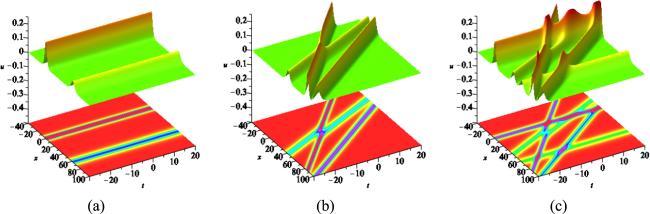
Figure 1. (a) Two-soliton, (b) three-soliton, and (c) their linear combination at y = 0, respectively.
We conclude this subsection with the following remarks:

1. The (n + 1)-component nonlinear integrable coupled KdV systems (47), featuring n sources, are non-decouplable. Decoupled systems only arise in the case of n = 1. It is important to emphasize that a significant consequence of the decoupled System I is that no individual KdV equation can serve as a solution to the pBKP equation (9). However, the sum of two arbitrary KdV equations does satisfy the pBKP equation. Specifically, neither w = c1w1 nor w = c2w2 in Proposition C is a solution to the pBKP equation (9) for any values of c1 and c2. However, the linear combination w = c1w1 + c2w2 does satisfy the pBKP equation. Therefore, the establishment of potential connections between integrable systems is achieved through the utilization of linear combinations. The non-decouplability of the (n + 1)-component coupled KdV systems highlights the importance of considering the collective behavior of multiple soliton solutions. The linear combination approach provides a powerful tool for constructing solutions that exhibit novel properties and can satisfy nonlinear integrable equations such as the pBKP equation. This approach expands our understanding of the interplay between different integrable systems and opens up new avenues for investigating their connections and dynamics.

2. Additional conditions need to be fulfilled by the parameters involved in Proposition C to ensure the validity of the desired linear superposition solutions of the pBKP equation (9). It is evident that both the first two decompositions presented in Proposition 1 and the known linear superpositions described in Proposition 2 are encompassed within Proposition C by choosing specific values for c1 and c2. The inclusion of these specific linear superpositions within Proposition C implies that the parameters c1 and c2 must satisfy certain conditions to ensure that the resulting solution is a valid solution of the pBKP equation. By carefully selecting appropriate values for these parameters, the linear combination of the individual solutions can yield a solution that satisfies the nonlinear integrable pBKP equation. Thus, Proposition C provides a more general framework that encompasses both the decompositions discussed in Proposition 1 and the known linear superpositions mentioned in Proposition 2. It highlights the importance of considering the specific values of c1 and c2 to ensure the desired linear superposition solutions are valid solutions of the pBKP equation.

3. By harnessing the power of integrable couplings, we can explore the intricate interplay and interdependence among different integrable systems. This methodology allows us to leverage the existing knowledge of solutions and properties from one system to obtain previously undiscovered solutions for other interconnected systems. In the context of the pBKP equation, the application of integrable couplings facilitates the derivation of hitherto unknown solutions, thereby expanding the repertoire of available solutions and enriching our comprehension of the equation's dynamical behavior.

3.2. Multi-component decompositions of the seventh-order pBKP equation (10)

The same principles and techniques employed in the analysis of the fifth-order pBKP equation can be applied to the seventh-order case. In a manner analogous to the computation of the multi-component decompositions of the seventh-order pBKP equation (10), similar assertions can be made.
Proposition D. Suppose w satisfies the nonlinear integrable couplings
$\begin{eqnarray}\begin{array}{rcl}{v}_{y} & = & {{\rm{\Phi }}}_{1}{v}_{x}+b,\\ \Space{0ex}{0.24em}{0ex}{w}_{y} & = & {{\rm{\Phi }}}_{2}{w}_{x}+2{{av}}_{x}(\displaystyle \frac{a}{3}{v}_{x}-{w}_{x})+c,\end{array}\end{eqnarray}$
and
$\begin{eqnarray}\begin{array}{rcl}{v}_{t} & = & 27{{\rm{\Phi }}}_{1}^{3}{v}_{x}+63c{{\rm{\Phi }}}_{1}{v}_{x}+{{dv}}_{x}+f,\\ {w}_{t} & = & 27{{\rm{\Phi }}}_{2}^{3}{w}_{x}-126a{{\rm{\Phi }}}_{2}^{2}{w}_{x}+63c{{\rm{\Phi }}}_{2}{w}_{x}+\displaystyle \frac{70}{3}{a}^{4}{v}_{x}^{4}\\ & & -140{a}^{3}{v}_{x}^{3}{w}_{x}+42{a}^{2}(15{v}_{x}^{2}{w}_{x}^{2}\\ & & +10{w}_{{xx}}{v}_{{xx}}{v}_{x}+5{w}_{x3}{v}_{x}^{2}+5{w}_{x}{v}_{{xx}}^{2}+10{v}_{x3}{w}_{x}{v}_{x}\\ & & +{{cv}}_{x}^{2}+4{v}_{{xx}}{v}_{x4}+2{v}_{x}{v}_{x5}\\ & & +3{v}_{x3}^{2})-126a(10{v}_{{xx}}{w}_{x}{w}_{{xx}}+5{v}_{x3}{w}_{x}^{2}+{{cv}}_{x}{w}_{x}\\ & & +2{w}_{{xx}}{v}_{x4}+3{w}_{x3}{v}_{x3}+{w}_{x}{v}_{x5}\\ & & +2{w}_{x4}{v}_{{xx}})+{{dw}}_{x}+e,\end{array}\end{eqnarray}$
then, w also satisfies the seventh-order pBKP equation (10).
Proposition E. If w is a solution of the nonlinear integrable (n + 1)-component KdV system
$\begin{eqnarray}\begin{array}{rcl}{v}_{{iy}} & = & {v}_{{ix}3}+3{w}_{x}{v}_{{ix}}+{b}_{i},\\ {w}_{y} & = & {{\rm{\Phi }}}_{3}{w}_{x}+\displaystyle \sum _{i=1}^{n}{a}_{i}{v}_{{ix}}^{2}+a,\\ {v}_{{it}} & = & 27{v}_{{ix}7}+189({v}_{{ix}5}{w}_{x}+{v}_{{ix}}{w}_{x5})\\ & & +378({v}_{{ix}4}{w}_{{xx}}+{v}_{{ixx}}{w}_{x4})+945({v}_{{ix}}{w}_{x}{w}_{x3}\\ & & +{v}_{{ixx}}{w}_{x}{w}_{{xx}})+\displaystyle \frac{945}{2}({w}_{x}^{2}{v}_{{ix}3}+{v}_{{ix}}{w}_{{xx}}^{2}\\ & & +{w}_{x}^{3}{v}_{{ix}})+567{v}_{{ix}3}{w}_{x3}+63{{av}}_{{ix}3}\\ & & +189{{av}}_{{ix}}{w}_{x}+{{bv}}_{{ix}}+{c}_{i}+315{a}_{i}{v}_{{ix}}({v}_{{ix}}{v}_{{ix}3}\\ & & +{v}_{{ixx}}^{2}+{v}_{{ix}}^{2}{w}_{x})\\ & & +63\displaystyle \sum _{j\ne i}^{n}{a}_{j}({v}_{{ix}3}{v}_{{jx}}^{2}+2{v}_{{ixx}}{v}_{{jx}}{v}_{{jxx}}+3{v}_{{ix}}{v}_{{jxx}}^{2}\\ & & +4{v}_{{ix}}{v}_{{jx}}{v}_{{jx}3}+5{v}_{{ix}}{v}_{{jx}}^{2}{w}_{x}),\\ {w}_{t} & = & 27{{\rm{\Phi }}}_{3}^{3}{w}_{x}+63a{{\rm{\Phi }}}_{3}{w}_{x}+{{bw}}_{x}+d+\displaystyle \frac{105}{2}\displaystyle \sum _{i=1}^{n}{a}_{i}^{2}{v}_{{ix}}^{4}\\ & & +63\displaystyle \sum _{i=1}^{n}(2{v}_{{ix}}{v}_{{ix}5}+4{v}_{{ixx}}{v}_{{ix}4}+3{v}_{{ix}3}^{2}\\ & & +{{av}}_{{ix}}^{2}+5{v}_{{ix}}^{2}{w}_{x3}+10{v}_{{ix}}{v}_{{ixx}}{w}_{{xx}}\\ & & +5(2{v}_{{ix}}{v}_{{ix}3}+{v}_{{ixx}}^{2}){w}_{x}+\displaystyle \frac{15}{2}{v}_{{ix}}^{2}{w}_{x}^{2})\\ & & +105\displaystyle \sum _{i\lt j}^{n}{a}_{i}{a}_{j}{v}_{{ix}}^{2}{v}_{{jx}}^{2},\end{array}\end{eqnarray}$
then, w is also a solution of the seventh-order pBKP equation (10).
Proposition F. Assuming that w1 and w2 represent compatible solutions of two independent KdV systems
$\begin{eqnarray}\begin{array}{rcl}{w}_{1y} & = & {{\rm{\Phi }}}_{4}{w}_{1x}-{\beta }_{1}{w}_{1x}+\mu ,\\ {w}_{2y} & = & {{\rm{\Phi }}}_{5}{w}_{2x}+{\beta }_{1}{w}_{2x}+{\mu }_{1},\\ {w}_{1t} & = & 27{{\rm{\Phi }}}_{4}^{3}{w}_{1x}-63{\beta }_{1}{{\rm{\Phi }}}_{4}^{2}{w}_{1x}\\ & & +(42{\beta }_{1}^{2}+63{c}_{1}\mu +63{c}_{2}{\mu }_{1}){{\rm{\Phi }}}_{4}{w}_{1x}-(7{\beta }_{1}^{3}\\ & & +126{c}_{1}\mu {\beta }_{1}){w}_{1x}+\delta ,\\ {w}_{2t} & = & 27{{\rm{\Phi }}}_{5}^{3}{w}_{2x}+63{\beta }_{1}{{\rm{\Phi }}}_{5}^{2}{w}_{2x}\\ & & +(42{\beta }_{1}^{2}+63{c}_{1}\mu +63{c}_{2}{\mu }_{1}){{\rm{\Phi }}}_{5}{w}_{2x}+(7{\beta }_{1}^{3}\\ & & +126{c}_{2}{\mu }_{1}{\beta }_{1}){w}_{2x}+{\delta }_{1},\end{array}\end{eqnarray}$
it can be established that the linear combination w = c1w1 + c2w2 serves as an exact solution to the seventh-order pBKP equation (10).
This intriguing result highlights the remarkable nature of the relationship between the solutions of the independent KdV systems and the seventh-order pBKP equation. It is worth noting that the first two decompositions presented in Proposition 3 and the known linear superpositions discussed in Proposition 4 can be viewed as specific instances of Proposition F by choosing particular values for c1 and c2. By considering appropriate values for the coefficients c1 and c2, this proposition allows for the derivation of a wide range of solutions that satisfy the seventh-order pBKP equation. This framework facilitates a deeper understanding of the interplay between different solutions and their relationship to the underlying dynamics of the system.

3.3. Multi-component decompositions of the ninth-order pBKP equation (11)

The findings in this subsection bear resemblance to the earlier results in terms of their properties and implications. The methodologies employed and the conclusions drawn share commonalities with those of the previous investigations.
Proposition G. If w represents a solution to the nonlinear integrable couplings
$\begin{eqnarray}\begin{array}{rcl}{v}_{y} & = & {{\rm{\Phi }}}_{1}{v}_{x}+b,\\ {w}_{y} & = & {{\rm{\Phi }}}_{2}{w}_{x}+2{{av}}_{x}(\displaystyle \frac{a}{3}{v}_{x}-{w}_{x})+c,\end{array}\end{eqnarray}$
and
$\begin{eqnarray*}\begin{array}{rcl}{v}_{t} & = & 81{{\rm{\Phi }}}_{1}^{4}{v}_{x}+243c{{\rm{\Phi }}}_{1}^{2}{v}_{x}+3{{\rm{\Phi }}}_{1}{v}_{x}+{{dv}}_{x}+e,\\ {w}_{t} & = & 81{{\rm{\Phi }}}_{2}^{4}{w}_{x}-486{{av}}_{x}{{\rm{\Phi }}}_{2}^{3}{w}_{x}+81(3c\\ & & +14{a}^{2}{v}_{x}^{2}){{\rm{\Phi }}}_{2}^{2}{w}_{x}-3(420{a}^{3}{v}_{x}^{3}+270{{acv}}_{x}\\ & & -1){{\rm{\Phi }}}_{2}{w}_{x}-486{{aw}}_{x}{{\rm{\Phi }}}_{1}^{3}{v}_{x}+420{a}^{4}(3{v}_{x}^{4}{w}_{x}\\ & & +2{v}_{x}^{3}{v}_{x3}+3{v}_{x}^{2}{v}_{{xx}}^{2}){a}^{4}-3780{a}^{3}{w}_{{xx}}{v}_{x}^{2}{v}_{{xx}}\end{array}\end{eqnarray*}$$\begin{eqnarray}\begin{array}{rcl} & & +2{a}^{2}(162{v}_{x}{v}_{x7}+486{v}_{{xx}}{v}_{x6}\\ & & +54(42{v}_{x}{w}_{x}+19{v}_{x3}){v}_{x5}\\ & & +621{v}_{x4}^{2}+2268({v}_{x}{w}_{{xx}}\\ & & +2{w}_{x}{v}_{{xx}}){v}_{x4}+2268{v}_{x}{v}_{{xx}}{w}_{x4}+3402{w}_{x}{v}_{x3}^{2}\\ & & +54(63{v}_{x}{w}_{x3}+77{w}_{{xx}}{v}_{{xx}}+(105{w}_{x}^{2}\\ & & +5c){v}_{x}){v}_{x3}+2079{v}_{{xx}}^{2}{w}_{x3}+135(21{w}_{x}^{2}+c){v}_{{xx}}^{2}\\ & & +11340{v}_{x}{w}_{x}{v}_{{xx}}{w}_{{xx}}+405{{cw}}_{x}{v}_{x}^{2}\\ & & +{v}_{x}^{2})-6a(243{w}_{{xx}}{v}_{x6}+243{v}_{{xx}}{w}_{x6}+27(21{w}_{x}^{2}\\ & & +19{w}_{x3}){v}_{x5}+513{v}_{x3}{w}_{x5}\\ & & +27(84{w}_{x}{w}_{{xx}}+23{w}_{x4}){v}_{4x}+2268{v}_{{xx}}{w}_{x}{w}_{x4}\\ & & +27(70{w}_{x}^{3}+126{w}_{x}{w}_{x3}+5{{cw}}_{x}\\ & & +77{w}_{{xx}}^{2}){v}_{x3}+4158{v}_{{xx}}{w}_{{xx}}{w}_{x3}+135(42{w}_{x}^{2}+c){w}_{{xx}}{v}_{{xx}}\\ & & +{v}_{x}{w}_{x})+{{dw}}_{x}+f,\end{array}\end{eqnarray}$
it can be inferred that w also serves as a solution to the ninth-order pBKP equation (11).
Proposition H. Let v and w be compatible solutions of the nonlinear coupled KdV system
$\begin{eqnarray}\begin{array}{rcl}{v}_{y} & = & {v}_{x3}+3{w}_{x}{v}_{x}+{b}_{1},\\ {w}_{y} & = & {{\rm{\Phi }}}_{3}{w}_{x}+{a}_{1}{v}_{x}^{2}+a,\\ {v}_{t} & = & 81{v}_{x9}+243(3{v}_{x7}{w}_{x}+3{v}_{x}{w}_{x7}+9{v}_{x6}{w}_{{xx}}\\ & & +9{v}_{{xx}}{w}_{x6}+19{v}_{x5}{w}_{x3}+19{v}_{x3}{w}_{x5}\\ & & +23{v}_{x4}{w}_{x4})+1701(3{v}_{x}{w}_{x}{w}_{x5}+6{v}_{x}{w}_{{xx}}{w}_{x4}\\ & & +6{w}_{x}{v}_{{xx}}{v}_{x4}+6{w}_{x}{v}_{x4}{w}_{{xx}}\\ & & +9{w}_{x}{v}_{x3}{w}_{x3}+11{v}_{{xx}}{w}_{{xx}}{w}_{x3})\\ & & +\displaystyle \frac{1701}{2}(3{w}_{x}^{2}{v}_{x5}+5{v}_{x3}{w}_{x}^{3}+9{v}_{x}{w}_{x3}^{2}+11{w}_{{xx}}^{2}{v}_{x3}\\ & & +\displaystyle \frac{15}{4}{v}_{x}{w}_{x}^{4})+e({v}_{x3}+3{v}_{x}{w}_{x})\\ & & +\displaystyle \frac{25515}{2}({v}_{{xx}}{w}_{x}^{2}{w}_{{xx}}+{v}_{x}{w}_{x}{w}_{{xx}}^{2}\\ & & +{v}_{x}{w}_{x}^{2}{w}_{x3})+{{bv}}_{x}\\ & & +\displaystyle \frac{567}{2}{a}_{1}^{2}{v}_{x}^{5}+567{a}_{1}(3{v}_{x}^{2}{v}_{x5}\\ & & +5{v}_{x}^{3}{w}_{x3}+9{v}_{x}{v}_{x3}^{2}+11{v}_{x3}{v}_{{xx}}^{2}+12{v}_{x}{v}_{{xx}}{v}_{x4}\\ & & +15{v}_{x}^{2}{v}_{x3}{w}_{x}+15{v}_{x}^{2}{v}_{{xx}}{w}_{{xx}}+15{v}_{x}{v}_{{xx}}^{2}{w}_{x}\\ & & +\displaystyle \frac{15}{2}{v}_{x}^{3}{w}_{x}^{2})+81a(3{v}_{x5}+5{a}_{1}{v}_{x}^{3}\\ & & +15{v}_{x3}{w}_{x}+15{v}_{{xx}}{w}_{{xx}}+15{v}_{x}{w}_{x3}+\displaystyle \frac{45}{2}{v}_{x}{w}_{x}^{2}),\\ {w}_{t} & = & 81{{\rm{\Phi }}}_{3}^{4}{w}_{x}+243a{{\rm{\Phi }}}_{3}^{2}{w}_{x}+e{{\rm{\Phi }}}_{3}{w}_{x}\\ & & +{{bw}}_{x}+d+\displaystyle \frac{945}{2}{a}_{1}^{2}{v}_{x}^{2}(3{v}_{x}^{2}{w}_{x}+4{v}_{x}{v}_{x3}\\ & & +6{v}_{{xx}}^{2})\\ & & +{a}_{1}[81(6{v}_{x}{v}_{x7}+18{v}_{{xx}}{v}_{x6}+38{v}_{x3}{v}_{x5}\\ & & +23{v}_{x4}^{2})+\displaystyle \frac{8505}{2}({v}_{x}^{2}{w}_{x}^{3}+{v}_{x}^{2}{w}_{{xx}}^{2}\\ & & +{v}_{{xx}}^{2}{w}_{x}^{2})\\ & & +8505({v}_{x}^{2}{w}_{x}{w}_{x3}+{v}_{x}{v}_{x3}{w}_{x}^{2})+567(3{v}_{x}^{2}{w}_{x5}\\ & & +9{v}_{x3}^{2}{w}_{x}+11{v}_{{xx}}^{2}{w}_{x3})\\ & & +1134(3{v}_{x}{v}_{x5}{w}_{x}+6{v}_{x}{v}_{{xx}}{w}_{x4}+6{v}_{x}{v}_{x4}{w}_{{xx}}\\ & & +6{v}_{{xx}}{v}_{x4}{w}_{x}+9{v}_{x}{v}_{x3}{w}_{x3}\\ & & +11{v}_{{xx}}{v}_{x3}{w}_{{xx}})+17010{v}_{x}{v}_{{xx}}{w}_{x}{w}_{{xx}}+405a({v}_{{xx}}^{2}\\ & & +2{v}_{x}{v}_{x3}+3{v}_{x}^{2}{w}_{x})+{{ev}}_{x}^{2}],\end{array}\end{eqnarray}$
then, w solves the ninth-order pBKP equation (11) as well.
Proposition I. Assuming that w1 and w2 are solutions of two independent KdV equations
$\begin{eqnarray}\begin{array}{rcl}{w}_{1y} & = & {{\rm{\Phi }}}_{4}{w}_{1x}-{\beta }_{1}{w}_{1x}+\mu ,\\ {w}_{2y} & = & {{\rm{\Phi }}}_{5}{w}_{2x}+{\beta }_{1}{w}_{2x}+{\mu }_{1},\\ {w}_{1t} & = & 81{{\rm{\Phi }}}_{4}^{4}{w}_{1x}-243{\beta }_{1}{{\rm{\Phi }}}_{4}^{3}{w}_{1x}+243({c}_{1}\mu \\ & & +{c}_{2}{\mu }_{1}+{\beta }_{1}^{2}){{\rm{\Phi }}}_{4}^{2}{w}_{1x}-90{\beta }_{1}({\beta }_{1}^{2}\\ & & +9{c}_{1}\mu ){{\rm{\Phi }}}_{4}{w}_{1x}-810{c}_{2}{\mu }_{1}{\beta }_{1}^{2}{w}_{1x}+\delta ,\\ {w}_{2t} & = & 81{{\rm{\Phi }}}_{5}^{4}{w}_{2x}+243{\beta }_{1}{{\rm{\Phi }}}_{5}^{3}{w}_{2x}+243({c}_{1}\mu \\ & & +{c}_{2}{\mu }_{1}+{\beta }_{1}^{2}){{\rm{\Phi }}}_{5}^{2}{w}_{2x}+90{\beta }_{1}({\beta }_{1}^{2}\\ & & +9{c}_{2}{\mu }_{1}){{\rm{\Phi }}}_{5}{w}_{2x}-810{c}_{1}\mu {\beta }_{1}^{2}{w}_{2x}+{\delta }_{1},\end{array}\end{eqnarray}$
it can be concluded that w = c1w1 + c2w2 satisfies the ninth-order pBKP equation (11).
It should be noted that the first two decompositions presented in Proposition 5 and the known linear superpositions discussed in Proposition 6 can be regarded as specific instances of Proposition I by selecting particular values for c1 and c2. Furthermore, all propositions presented in this paper have been rigorously verified through direct calculation. The validity and accuracy of the results have been established by performing detailed computations and verifying the consistency of the derived equations. Considering the success of the decompositions utilized in this paper, it is natural to consider extending these decomposition techniques to encompass the entire pBKP hierarchy. By generalizing the argument, we propose that for each equation within the pBKP hierarchy, multi-component decompositions exist that enable the representation of solutions in terms of multiple components. Additionally, we conjecture the existence of a special general linear superposition that allows for the combination of these decomposed solutions.

4. Conclusions and discussions

This research paper serves as a catalyst for investigating the multi-component decompositions and linear superpositions within the context of the nonlinear pBKP hierarchy. The primary focus of this study centers around the development of innovative multi-component decompositions for three specific pBKP equations, achieved through the enlargement of the spectral problem. These decompositions enable the derivation of novel nonlinear integrable coupled KdV-type systems with n sources, exhibiting an abundance of higher-order symmetries. Additionally, a general linear combination solution is constructed, establishing a connection to two arbitrary KdV couplings. The propositions presented in this paper, labeled as Propositions A-I, offer distinct decompositions of the pBKP equations. These decompositions play a pivotal role in constructing extensive classes of solutions for the pBKP equations, utilizing the solutions derived from these decompositions. Notably, the linear superpositions outlined in Proposition 2, 4 and 6 can be viewed as specific instances of Proposition C, F and I with particular parameter choices. It is important to recognize the significance of these findings, as they contribute to the understanding and exploration of the pBKP hierarchy. By employing multi-component decompositions and exploiting the relationships between different solutions, a rich variety of solutions for the pBKP equations can be obtained. Furthermore, the identification of special cases within the linear superpositions highlights the versatility and applicability of the proposed decomposition techniques. The results presented in this paper lay the foundation for further investigations in this field. Future research endeavors can focus on extending these decompositions and superposition techniques to other equations, as well as exploring their connections to other integrable systems.
Within the framework established in this paper, it is anticipated that a plethora of integrable multi-component decompositions for high-dimensional nonlinear systems can be unveiled. Furthermore, while various methods exist for solving nonlinear PDEs, it can be argued that the novel decomposition method employed in this study offers a relatively straightforward approach for obtaining exact solutions for a broad range of nonlinear PDEs without the need for linearization or restrictive assumptions. In comparison to other exact methods, this approach often provides a more accessible means of finding exact solutions. In certain cases, this decomposition method enables the identification of classes of solutions for a given nonlinear PDE through the direct application of the method to the equation. This includes the possibility of discovering linear combination solutions that encompass linear superposition solutions. Currently, the expressions and techniques associated with linear superposition in nonlinear theory are in a nascent stage, lacking a comprehensive theoretical framework. Thus, there is a need for further exploration and analysis to uncover additional examples of nonlinear equations for which the solutions adhere to the principle of linear superposition. Ultimately, the aim is to develop a systematic theory that encompasses the principles and methods of linear superposition in the context of nonlinear equations. In light of recent experimental observations of soliton interactions, as reported in [44, 45], our theoretical findings may offer valuable insights for future experimental designs and interpretations. These studies highlight the practical relevance of our theoretical models and suggest that our decomposition techniques could be instrumental in the experimental investigation of soliton dynamics.
By advancing our understanding of multi-component decompositions and linear superposition in nonlinear systems, this research opens up new avenues for tackling complex high-dimensional nonlinear problems. The insights gained from this study can contribute to the development of more efficient and effective solution techniques, ultimately deepening our comprehension of the underlying mathematical structures and paving the way for future advancements in the field of nonlinear PDEs.

The work was sponsored by the National Natural Science Foundations of China under Grant Nos. 12301315, 12235007, 11975131, and the Zhejiang Provincial Natural Science Foundation of China under Grant No. LQ20A010009.

1
Fan E G 2002 Solving Kadomtsev–Petviashvili equation via a new decomposition and Darboux transformation Commun. Theor. Phys. 37 145 148

DOI

2
Lou S Y, Hu X B 1998 Broer-Kaup Systems from Darboux Transformation Related Symmetry Constraints of Kadomtsev-Petviashvili Equation Commun. Theor. Phys. 29 145 148

DOI

3
Konopelchenko B G, Schief W K, Szereszewski A 2021 Self-dual Einstein spaces and the general heavenly equation. Eigenfunctions as coordinates Class. Quantum Grav. 38 045007

DOI

4
Lou S Y, Chen L L 1999 Formal variable separation approach for nonintegrable models J. Math. Phys. 40 6491 6500

DOI

5
Lou S Y, Tang X Y, Lin J 2001 Exact solutions of the coupled KdV system via a formally variable separation approach Commun. Theor. Phys. 36 145 148

DOI

6
Chen Y, X 2023 Wronskian solutions and linear superposition of rational solutions to B-type Kadomtsev–Petviashvili equation Phys. Fluids 35 106613

DOI

7
Hu H C, Li X D 2022 Nonlocal symmetry and interaction solutions for the (3.1)-dimensional interable Boussinesq equation Math. Model. Nat. Phenom. 17 1 10

DOI

8
Lou S Y, Hao X Z 2022 Linear superposition in the general heavenly equation Phys. Lett. A 443 128203

DOI

9
Ma W X 2021 A polynomial conjecture connected with rogue waves in the KdV equation Part. Differ. Eq. in Appl. Math 3 100023

DOI

10
Mahajan S, Miura H 2009 Linear superposition of nonlinear waves J. Plasma Phys. 75 145 152

DOI

11
Ponomarenko S A 2002 Linear superposition principle for partially coherent solitons Phys. Rev. E 65 055601

DOI

12
Zhang Z A, Lou S Y 2023 Linear superposition for a sine-gordon equation with some types of novel nonlocalities Phys. Scr. 98 035211

DOI

13
Hao X Z, Lou S Y 2022 Decompositions and linear superpositions of B-type Kadomtsev–Petviashvili equations Math. Meth. Appl. Sci. 45 5774 5796

DOI

14
Li Y, Yao R X, Xia Y R, Lou S Y 2021 Plenty of novel interaction structures of soliton molecules and asymmetric solitons to (2.1)-dimensional Sawada–Kotera equation Commun. Nonlinear Sci. Numer. Simulat. 100 105843

DOI

15
Yao R X, Li Y, Lou S Y 2021 A new set and new relations of multiple soliton solutions of (2.1)-dimensional Sawada–Kotera equation Commun. Nonlinear Sci. Numer. Simulat. 99 105820

DOI

16
Konopelchenko B G, Dubrovsky V G 1984 Some new integrable nonlinear evolution equations in 2+1 dimensions Phys. Lett. A 102 15 17

DOI

17
Cheng Y, Li Y S 1992 Constraints of the 2.1 dimensional integrable soliton systems J. Phys. A: Math. Gen. 25 419 431

DOI

18
Fuchssteiner B 1983 Mastersymmetries, higher order time-dependent symmetries and conserved densities of nonlinear evolution equations Prog. Theor. Phys. 70 1508 1522

DOI

19
Cao C W 1990 Nonlinearization of the Lax system for AKNS hierarchy Sci. China A 33 528 536

DOI

20
Cao C W, Geng X G 1990 Classical integrable systems generated through nonlinearization of eigenvalue problems Nonlinear Phys. 68 78

DOI

21
Cao C W, Geng X G 1990 Neumann and Bargmann systems associated with the coupled KdV soliton hierarchy J. Phys. A: Math. Gen. 23 4117 4125

DOI

22
Cheng Y, Li Y S 1991 The constraint of the Kadomtsev–Petviashvili equation and its special solutions Phys. Lett. A 157 22 26

DOI

23
Geng X G, Cao C W 1999 Quasi-periodic solutions of the 2+1 dimensional modified Korteweg–de Vries equation Phys. Lett. A 261 289 296

DOI

24
Sidorenko J, Strampp W 1993 Multicomponent integrable reductions in the Kadomtsev–Petviashvilli hierarchy J. Math. Phys. 34 1429 1446

DOI

25
Geng X G, Cao C W 2001 Decomposition of the (2.1)-dimensional Gardner equation and its quasi-periodic solutions Nonlinearity 14 1433 1452

DOI

26
Lou S Y, Huang F 2017 Alice-Bob physics: coherent solutions of nonlocal KdV systems Sci. Rep. 7 1 11

DOI

27
Lou S Y, Qiao Z J 2017 Alice-Bob peakon systems Chinese Phys. Lett. 34 100201

DOI

28
Qu C Z, Song J F, Yao R X 2013 Multi-component integrable systems and invariant curve flows in certain geometries SIGMA 9 1 19

DOI

29
Swarup S, Vasan V, Kulkarni M 2020 Provable bounds for the Korteweg–de Vries reduction in multi-component nonlinear Schrödinger equation J. Phys. A: Math. Theor. 53 135206

DOI

30
Foursov M V 2000 Classification of certain integrable coupled potential KdV and modified KdV-type equations J. Math. Phys. 41 6173 6185

DOI

31
Hu H C, Tong B, Lou S Y 2006 Nonsingular positon and complexiton solutions for the coupled KdV system Phys. Lett. A 351 403 412

DOI

32
Qian S P, Tian L X 2007 Nonlocal Lie-Bäcklund symmetries of the coupled KdV system Phys. Lett. A 364 235 238

DOI

33
Xia Y R, Yao R X, Xin X P, Li Y 2021 Nonlocal symmetry, Painlevé integrable and interaction solutions for CKdV equations Symmetry 13 1268

DOI

34
Lou S Y, Tong B, Hu H C, Tang X Y 2006 Coupled KdV equations derived from two-layer fluids J. Phys. A: Math. Gen. 39 513 527

DOI

35
Liang Z F, Tang X Y, Ding W 2021 Infinitely many nonlocal symmetries and nonlocal conservation laws of the integrable modified KdV-sine-Gordon equation Commun. Theor. Phys. 73 055003

DOI

36
Lou S Y, Hu X B 1994 Infinitely many symmetries of the Davey–Stewartson equation J. Phys. A: Math. Gen. 27 L207 L212

DOI

37
Ma W X, Xu X X, Zhang Y F 2006 Semi-direct sums of Lie algebras and continuous integrable couplings Phys. Lett. A 351 125 130

DOI

38
Olver P J 1977 Evolution equations possessing infinitely many symmetries J. Math. Phys. 18 1212 1215

DOI

39
Alexandrov A 2021 KdV solves BKP P. Natl. Acad. Sci. 118 e2101917118

DOI

40
Lou S Y 2020 Soliton molecules and asymmetric solitons in three fifth order systems via velocity resonance J. Phys. Commun. 4 041002

DOI

41
Sawada K, Kotera T 1974 A method for finding N-soliton solutions of the KdV equation and KdV-like equation Prog. Theor. Phys. 51 1355 1367

DOI

42
Yu W T, Liu W J, Zhang H X 2022 Soliton molecules in the kink, antikink and oscillatory background Chaos Soliton Fract. 159 112132

DOI

43
Zhang R F, Bilige S D 2019 Bilinear neural network method to obtain the exact analytical solutions of nonlinear partial differential equations and its application to p-gBKP equatuon Nonlinear Dyn. 95 3041 3048

DOI

44
Si Z Z, Wang D L, Zhu B W, Ju Z T, Wang X P, Liu W, Malomed B A, Wang Y Y, Dai C Q 2024 Deep Learning for dynamic modeling and coded information storage of vector-soliton pulsations in mode-locked fiber lasers Laser Photon. Rev. 2400097

DOI

45
Si Z Z, Wang Y Y, Dai C Q 2024 Switching, explosion, and chaos of multi-wavelength soliton states in ultrafast fiber lasers Sci. China Phys. Mech. Astron. 67 274211

DOI

Outlines

/